Android Malware Detection Using Machine Learning with Feature Selection Based on the Genetic Algorithm

Abstract

Since the discovery that machine learning can be used to effectively detect Android malware, many studies on machine learning-based malware detection techniques have been conducted. Several methods based on feature selection, particularly genetic algorithms, have been proposed to increase the performance and reduce costs. However, because they have yet to be compared with other methods and their many features have not been sufficiently verified, such methods have certain limitations. This study investigates whether genetic algorithm-based feature selection helps Android malware detection. We applied nine machine learning algorithms with genetic algorithm-based feature selection for 1104 static features through 5000 benign applications and 2500 malwares included in the Andro-AutoPsy dataset. Comparative experimental results show that the genetic algorithm performed better than the information gain-based method, which is generally used as a feature selection method. Moreover, machine learning using the proposed genetic algorithm-based feature selection has an absolute advantage in terms of time compared to machine learning without feature selection. The results indicate that incorporating genetic algorithms into Android malware detection is a valuable approach. Furthermore, to improve malware detection performance, it is useful to apply genetic algorithm-based feature selection to machine learning.

1. Introduction

Since AndroidOS.DrioidSMS.A, the first malicious Android application was discovered in August 2010 [1], the discovery of additional Android malware has steadily increased. Based on this, the anti-malware software company Kaspersky [2] reported 5,683,694 malicious applications in 2020, the highest figure during the last 3 years. With the expected increase in the growth of malicious applications, along with the influence of Android OS, which boasted a 72.72% share globally as of May 2021 [3], it is necessary to develop a solution that can protect users by detecting malicious applications and blocking access before the damage becomes critical.

To solve this problem, techniques for Android malware detection using static/dynamic analysis have emerged. As outlined by P. D. Sawle and A. B. Gadichi [4], several studies have proposed various types of methods for Android malware detection, and many different analysis tools have been suggested and utilized. Owing to the limitations of traditional analytical techniques, detection using machine learning with static/dynamic features, and further detection through deep learning techniques, are spreading.

As a result, related studies on finding the best techniques have been conducted. K. Liu et al. [5] presented research on machine learning-based Android malware detection conducted up to the year 2020. In addition, Z. Wang et al. [6] published a review of Android malware detection applying deep learning. Rana et al. [7] also found an algorithm that best classifies malware through experiments, aiming to find the most effective malware detector among 12 different machine learning algorithms. Based on these results, anti-malware software and frameworks for the detection of real-world malicious applications have also been released. For example, M. Ahmedi et al. [8] proposed an IntelliAV system that detects malicious applications based on machine learning. They developed an anti-malware application that reported a better performance than commercial products and released it to the Google Play store (https://play.google.com/store/apps/details?id=com.intelliav (accessed on 8 May 2021)). A. Mahindru and A.L. Sangal [9] presented a framework named MLDroid. This showed a high detection rate of 98.8% through experiments with more than 500,000 applications based on several machine learning algorithms.

According to K. Liu et al. [5], many studies have applied feature selection with information gain, along with various methods for reducing the features used in machine learning, with the expectation of increasing the normalization performance and operational efficiency. These attempts are meaningful, because D. Ö. Şahin et al. [10] confirmed that feature selection could be successfully applied to detect Android malware based on the comparative experiments with various feature selection methods. However, S. Lei [11] indicated that all of these feature selection methods have certain limitations. Thus, research on applying feature selection using genetic algorithms, which are advanced in comparison to traditional methods, has emerged.

Since A. Firdaus et al. [12] first introduced Android malware detection with genetic selection based on the use of a genetic algorithm, A. Fatima et al. [13] conducted a study validating its performance by building a support vector machine and neural networks with 33∼40 features selected from among 99 features by applying genetic algorithms. O. Yildiz and I. A. Doğru [14] presented the experimental results of selecting 152 features from information of Android permission, choosing 16 features by applying genetic algorithm-based feature selection, and verified the performance using a decision tree, naïve Bayes, and a support vector machine. A. Meimandi et al. [15] showed a performance improvement by combining genetic algorithm and the simulated annealing with classification algorithm. J. Wang et al. [16] introduced SEdroid, an Android malware detector based on a genetic algorithm and ensemble learning. L. Wang et al. [17] introduced a new algorithm based on the genetic algorithm for applications of Android malware classification problems.

However, none of the studies mentioned proved that genetic algorithm-based feature selection is more effective than other methods. The authors did not show any comparisons with traditional experiments of feature selection. Moreover, A. Fatima et al. [13] demonstrated a decrease in accuracy when applying genetic algorithms. This result indicates that the challenge of verifying whether detection methods using genetic algorithms are efficacious compared to other methods was left for future studies. Furthermore, because most studies set the numbers of features to less than 200, it is necessary to verify whether performance improvements can be achieved even in feature sets in which the numbers of features are sufficiently large (approximately 1000 or more) when applying a genetic algorithm.

This study discusses whether it is efficient and valuable to apply machine learning using feature selection with genetic algorithms for Android malware detection as alternatives to existing methods. Based on the structure and analysis methods of Android applications and the contents of existing machine learning approaches to malicious application detection, we compare the performances of existing methods herein, reveal whether genetic algorithms help improve performance, and show which genetic algorithms can achieve enhancements. Furthermore, we experimentally examined whether feature selection based on a genetic algorithm is a competitive approach compared to other methods.

The remainder of this paper is organized as follows: Section 2 describes the structure and analysis method of Android applications. Section 3 introduces the machine learning techniques used in this study, with feature selection at the forefront. Section 4 describes the progress of the experiment, confirming the claims of this study. The results are then presented in Section 5. Finally, Section 6 presents the conclusions of the experiment.

2. Android Malware Analysis

2.1. Structure of Android Application

Android application files generally have an extension called APK, which is short for Android Package. The APK is a file that runs applications compressed in zip format and installed on the Android OS. The package ties up several files needed to run the program, and one can see a unique structure to the APK file after decompressing it. Figure 1 shows a schematic structure of the APK package.

Numerous studies describe the structure in the following manner [6,19,20]:

• Manifest: This area contains basic information regarding the application and is located at the root of all APK files under the name AndroidManifest.xml, a binary XML file containing the declarations of important information regarding the application, such as the package name, component, application permissions, and device compatibility.
• Signatures: This is the area containing the signature of the application. The META-INF directory, where the application signature files are located, is found in this area.
• Assets: Assets are used to store static files used in an application and are implemented as an asset directory, which requires invoking the AssetManager class to access files in the area when real-operating applications are used.
• Compiled Resources: It contains pre-compiled resource information, which exists as a resources.arsc file. This file is responsible for matching the resource files and resource IDs to record them such that resources can be found, accessed, and used within an application.
• Native libraries: These make up the area for the libraries used in an application. Library files tailored to the CPU instruction set of the target device are located at the lib directory, primarily written in C/C++.
• Dalvik bytecode: This area contains JAVA’s byte code. Within the application, it is implemented in the classes.dex file, and contains source code content compiled into bytecodes that Dalvik virtual machines can compile. Each application contains one DEX file as a default, but there are applications with multiple DEX files [21].
• Resources: This is the collection of resources used in an application. The resources of the Android application are saved in the res directory.

The areas to be looked at when detecting Android malware are the Manifest and Dalvik bytecode. The Manifest is a critical area within an APK file, where one can extract and analyze information such as the version number, permission, and functionality that the application requires [22]. Dalvik bytecode contains the main code of the application as bytecode compiled by the virtual machine. By analyzing it through decompile files, the analyzer can check which class and methods are used by the applications and where harmful codes are called. After all, these domains can be extracted from the features used for machine learning and directly affect the execution of the application. Therefore, Android application analysis focuses on the Manifest and Dalvik bytecode areas.

2.2. Static and Dynamic Analysis

Static analysis is an automatic method of reasoning regarding the runtime attributes of a program code without executing the program directly [23]. It relies on the source code and resources of the program for analysis without execution. This type of analysis can be divided into signature-based analysis, permission-based analysis, and virtual machine analysis. It is based on the reliance of analyzing the source code [24]. A static analysis of Android malware detection is applied using AndroidManifest.xml, smali files, and a set of static features including permissions, API calls, Dalvik opcode, and other components, which can be obtained by decompiling the APK files, the main objective for analysis [5]. It has an advantage in that it takes less time and does not have a higher computational load than a dynamic analysis. Moreover, it can analyze the entire code regardless of time, enabling efficient analysis, such as analyzing only the necessary parts. However, there are also disadvantages, in that an analysis is impossible if static elements cannot be appropriately extracted from the malware, and it is challenging to handle malicious code that has been processed complexly owing to obfuscations.

A dynamic analysis involves analyzing the properties of a running program [25]. To describe this in more detail, it is a method of running applications directly on an actual device or sandbox environment, monitoring to understand the behavior, and analyzing logs and the traffic obtained from them. All input traces generated by the user are collected through data collector applications, crowdsourcing, and data collection scripts [4]. The analyzer logs both the collected inputs and their results by collecting dynamic objects. The objects include system calls, API calls, network traffic, and CPU data from Android applications [5]. A dynamic analysis has the advantage of being able to detect malicious behavior that a static analysis cannot detect, handle malicious code using obfuscation technology, and analyze whether the application is running even when important content such as a signature is missing. Nevertheless, it takes more time for analysis and detection than static procedures and requires numerous resources. Furthermore, as M. Y. Wong and D. Lie noted [26], codes implementing a behavior can be used to detect malicious operations only if executed during analysis, resulting in the dynamic analysis wasting many computational cycles by analyzing irrelevant parts of the application.

As shown in

Table 1. A summary of static and dynamic analysis.

Analysis Method	Static Analysis	Dynamic Analysis
Target of analysis	Source code and program components	Logs, traffic obtained by program execution
Pros	– Requires less time – Consumes fewer resources – Enables an effective analysis	– Is able to detect hidden malicious operations – Can handle obfuscated malware – Can be analyzed if the runnable
Cons	– Cannot be used for malicious codes that are unable to extract static elements – Has difficulty analyzing complex processed malware such as obfuscations	– Takes a significant amount of time – Consumes more resources – Can analyze only executed content, which is inefficient when executing unrelated parts

, static and dynamic analyses have a complementary relationship. The shortcomings of a static analysis can be solved by introducing a dynamic analysis, and the defects of a dynamic analysis can be supplemented with a static analysis. It is therefore impossible to determine which of these two analyses is better, and it is necessary to use appropriate methods depending on the detection purpose and environment. Of course, choosing features for machine learning should also be selected when considering these points. The flaws in the dynamic analysis are highlighted in this regard. As previously mentioned, it is necessary to obtain the results from running the application process directly during the dynamic analysis. However, it is crucial to run all data in the dataset, and this problem becomes more challenging as the dataset grows. Therefore, we conducted machine learning with features obtained through static analysis in this study.

3. Machine Learning Techniques

3.1. Feature Selection

Feature selection is a technique applied in machine learning, which refers to selecting features relevant to predictive data and using them for learning. According to I. Guyon and A. Elisseeff [27], there are many potential benefits of variable and feature selection, including facilitating data visualization and data understanding, reducing the measurement and storage requirements, reducing the training and utilization times, and defying the curse of dimensionality to improve the prediction performance. This process differs from feature extraction, which has the same effect as feature selection. Feature extraction directly selects the feature associated with the model configuration, which projects the original high-dimensional feature into a low-feature dimension [28], which is different from a feature selection.

Feature selection is primarily classified into filter, wrapper, and embedded methods. A filter method consists of three main steps: feature set generation, measurement, and learning algorithms. It repeats the information measurements of a new set generation-feature set process until the termination conditions are satisfied [29]. Unlike a filter method, the wrapper method applies to select features through a black box that relies on a learning algorithm. When a feature set enters the black box, the most highly evaluated features are produced based on the results of the learning algorithm [30]. The embedded method conducts a feature selection during a training process and is usually specific to the given learning machines [27].

As it consumes fewer resources than when learning the original dataset, the machine learning performance will be improved if feature selection is appropriately applied even on the dataset specified in this study. However, according to A. Firdaus et al. [12], feature selection significantly affects the experimental results in malware detection. For greater effectiveness, it is therefore necessary to choose an excellent feature. When applying feature selection techniques in general, it is more effective for the chosen features to maximize the relationship between a selected feature set and the label to be predicted. By contrast, the relationship between the selected features must be minimized to avoid redundant information [31]. In this study, a genetic algorithm was used to select the optimal features that best meet the stated conditions.

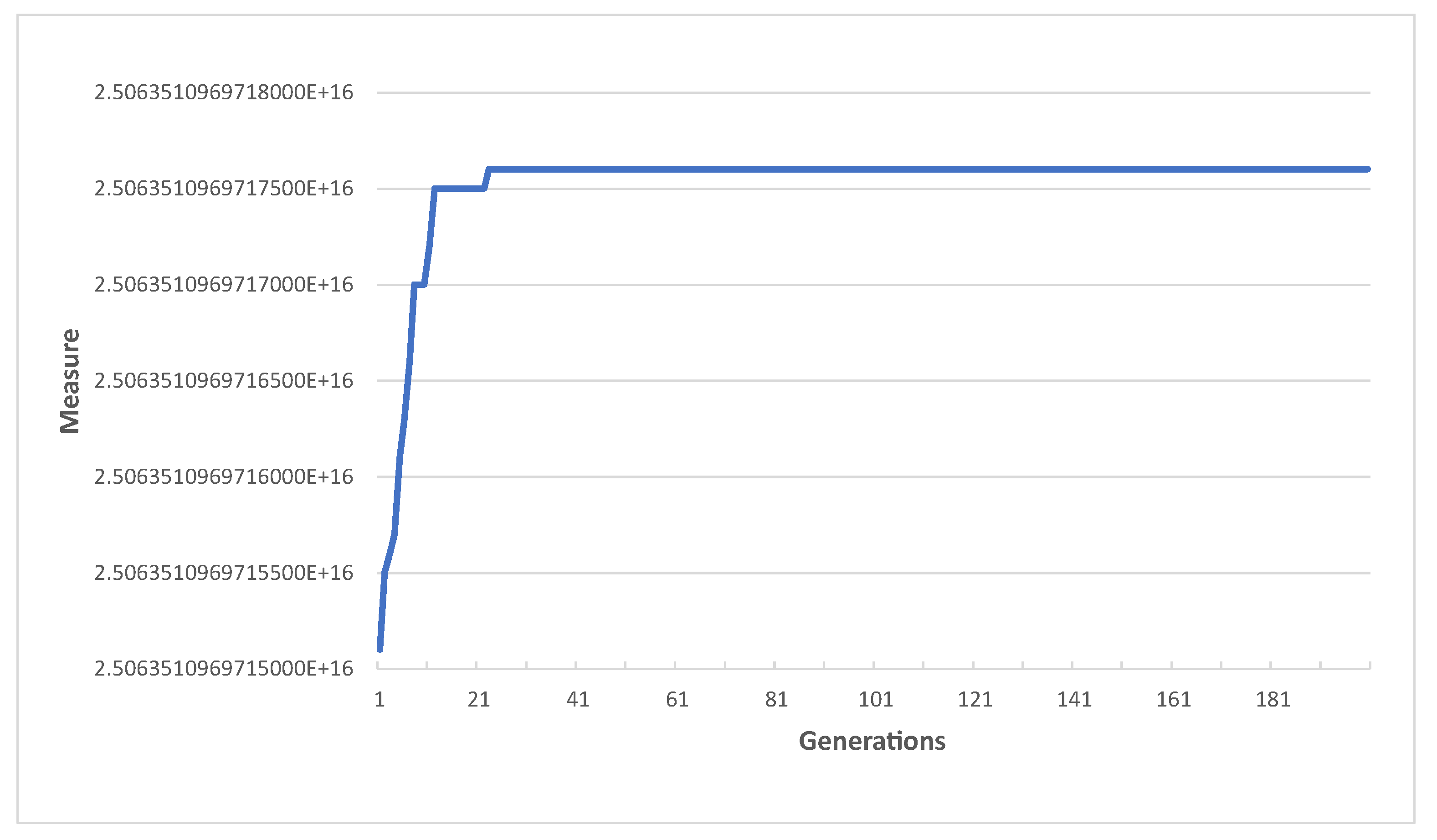
3.2. Genetic Algorithm

A genetic algorithm is based on biological evolution, as presented by Holland in 1975 [32]. Just as genes in nature partially crossover, mutate to create new genes that differ from existing ones, and evolve into an environment, genetic algorithms evolve objects through crossover and mutation procedures to find the optimized solutions. The solution found using a genetic algorithm converges in specific ways as the generations pass. The algorithm has disadvantages that cannot guarantee the required solution owing to the lack of standard rules governing it. In addition, the algorithm cannot guarantee the best solution because the solution only converges and does not progress, resulting in the solutions being poorly optimized [33]. However, it has the advantages of helping secure and explore potentially substantial search spaces, finding optimal combinations, and finding solutions that are difficult to achieve. Thus, it is suitable for finding an answer to an NP-hard problem, such as feature selection [34,35]. That means, it was also appropriate to apply a genetic algorithm in this study.

According to D. Whitley [36], a genetic algorithm usually begins with randomly generated gene populations. They evaluated the genes that were constructed and allocated opportunities for the next generation of each gene, such that the genes that met the problem’s criteria provided more chances of reproduction than those that did not. Subsequently, new genes were created by taking only the selected genes according to specific criteria and recombining them in many different ways. After creating new genes through a crossover, mutations can be created with specific probabilities. This process is repeated until the termination criteria of the algorithm are met. Figure 2 shows these procedures in a simplified flowchart.

3.3. Machine Learning Algorithm

Machine learning refers to computer programming used to optimize the performance criteria using example data or experience [37]. T. M. Mitchell [38] described machine learning as inherently a multidisciplinary field used in various real-world applications. Machine learning is conducted by introducing several algorithms to solve problems in various fields. This is the reason why machine learning must be evaluated through various algorithms. Thus, we selected nine algorithms to evaluate the performance of feature selection. The following descriptions are for the machine-learning algorithms used in this study.

• Decision Tree: A decision tree is a machine learning technique that classifies or regresses the data by creating classification rules for the trees. A decision tree is guided by a training case in which information is represented by a tuple and the class label of the attribute values is written down. Owing to the vast space to be retrieved, a tree is typically guided by training data and empty trees and into greedy, top-down, and recursive processes. The tree is created using processes that best partition the training data as the root splitting attribute. The training data are then partitioned into disjoint subsets that satisfy the values of the splitting attribute [39]. Owing to the disadvantage of easily overfitting the trees, pruning may be applied while executing the algorithm, or some trees might be removed to form generalized results.
• Random Forest: A random forest is a classifier consisting of a collection of uncorrelated tree structure classifiers designed by L. Breiman [40]. Each tree has the characteristic of finding solutions while voting for the most generalized class for input values. A supervised learning algorithm trained using the bagging method builds multiple decision trees and merges them to obtain a more accurate and stable prediction [7].
• Decision Table: A decision table is a simple means of documenting different decisions or actions taken under different sets of conditions [41]. The decision table allows the creation of a classifier, which summarizes the dataset into a decision table that contains the same number of attributes as the original dataset [42] and applies the classification of new incoming data using the table.
• Naïve Bayes: Naïve Bayes is a classification model based on the conditional probability of a Bayes rule. The independent naïve Bayes model is based on estimating and comparing probabilities; the larger significant probability points out that the actual label is more likely to be the class label value of the larger probability [14]. As the algorithm assumes that the predictive attributes are conditionally independent given the class, and it posits that no hidden or latent attributes influence the prediction process [43], it is difficult to apply to data dependent on different classes through specific attributes.
• MLP: A multi-layer perceptron (MLP) uses omnidirectional artificial neural networks for learning [44]. The neural network structure is presented in three parts: the input layer, hidden layer, and output layer. The input layer obtains the data, the hidden layer is calculated through an activation function, and the output layer shows the results of classification/regression. Although the input/output layers of the model exist individually, the hidden layer can be stacked as multiple layers. It is also known that the deeper a model is, the more generalized it can be in comparison to a shallowly stacked model [45].
• SVM: A support vector machine (SVM), also known as a support vector network (SVN), is a learning model for binary classification that embodies the idea that input vectors map non-linearly to high-dimensional feature spaces. In this feature space, a linear decision surface is constructed to ensure the high generalization ability of the learning machine owing to the unique properties of the decision surface [46].
• Logistic Regression: Logic regression is a machine learning technique that explains how variables with two or more categories are associated with a set of continuous or categorical predictors through probability functions [47]. Unlike ordinary linear regression using straight lines for classification, logistic regression is suitable for binary classification, using a logistic function in the shape of $\frac{e^x}{(1+e^x)}$ when fitting the data.
• AdaBoost: AdaBoost is a boosting algorithm that combines multiple weak classifiers to create a robust classifier that increases the performance. Unlike previously proposed boosting algorithms, a weak classifier is characterized by errors returned by the weak classifier [48], which affects the focus of the weak classifier on the problematic examples of the training set [49], allowing it to better classify the attributes.
• K-NN: As the fundamental principle of a K-nearest neighbor (K-NN), if most of the samples around the data on a point in a particular space belong to a specific category, the data on that point can be judged to fall into that category [50]. The K-NN algorithm operates by checking the label of the appropriate numbers of samples closest to the data being classified and subsequently labeling the data as the most aggregated of the samples.

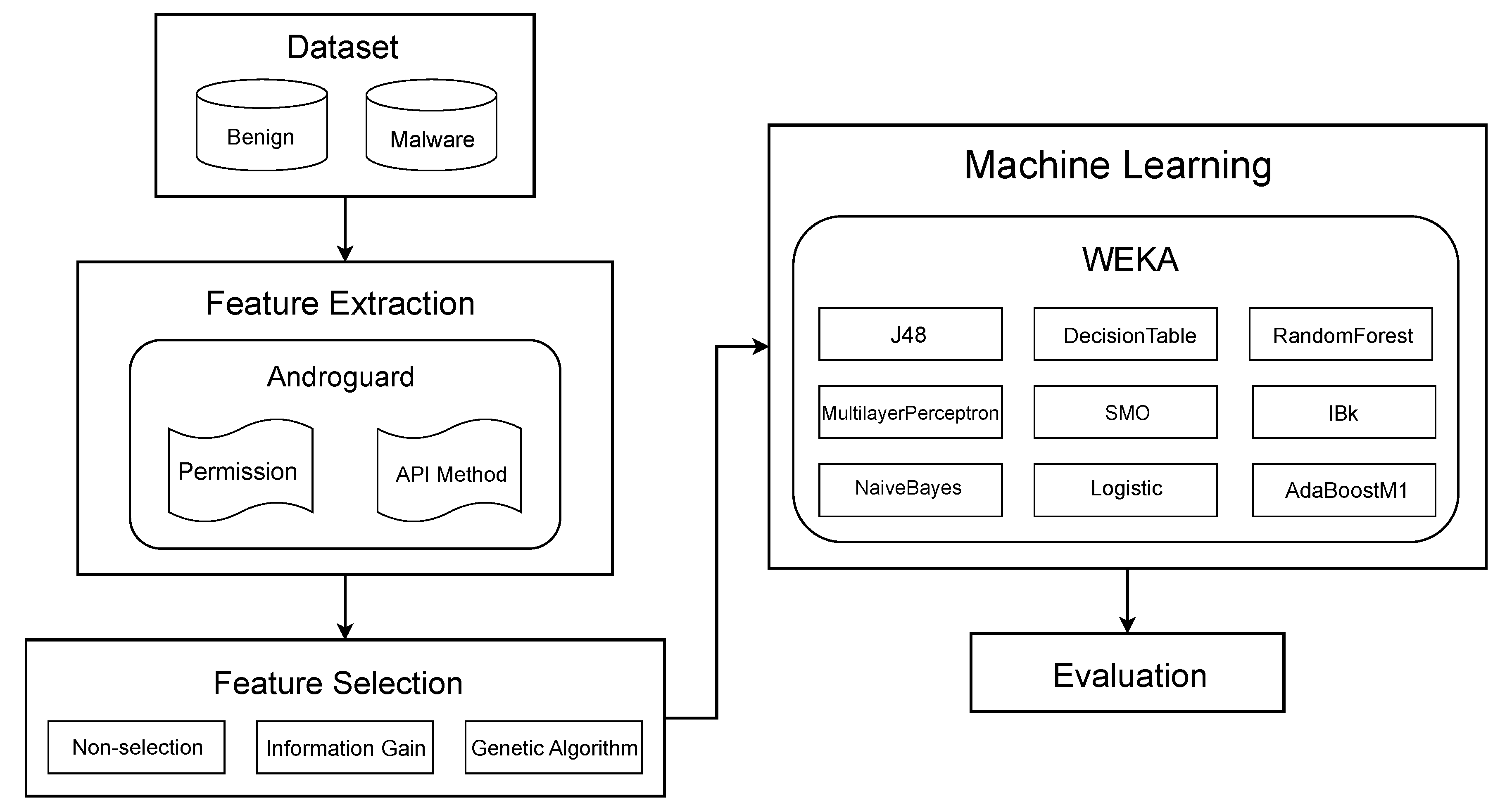
4. Experimental Methodology

In this section, the experiment conducted based on the flowchart in Figure 3 is described. During the experimental process, we used Androguard [51], a python-based Android application analysis tool for feature extraction; and WEKA [52], machine learning software provided by Waikato University for feature selection (information gain only), machine learning, and evaluation. In addition, the generation of a dataset for machine learning and the implementation of a genetic algorithm-based feature selection was conducted using Python scripts.

4.1. Dataset Selection and Modification

The dataset used in this experiment was modified from the Andro-AutoPsy Dataset  (https://ocslab.hksecurity.net/andro-autopsy (accessed on 11 May 2021)) [53] provided by the Hacking and Countermeasure Research Lab (HCRL), Korea University. The dataset consists of 9990 malicious and 109,193 benign applications collected between January 2013 and April 2014. We randomly selected and edited the attributes of this dataset to reduce the size of the dataset and divided them into training and test sets for machine learning.

Table 2. Distribution of attributes of datasets used in the experiment.

Class	Training	Test
Benign	4000	1000
Malware	2000	500

shows the distribution of attributes of the final modification of the dataset.

4.2. Initial Feature Extraction

A review by K. Liu et al. [5] confirms that 66 machine learning studies with static features mostly used application permissions or API calls. Many studies have combined multiple features to construct the learning data. Most studies used combination of permissions and API calls information. Therefore, we also decided on features based on combination of Android permissions and API calls and used them for machine learning during this experiment. Specifically, we obtained the permission information defined in the AndroidManifest.xml file and the API class method called in the application and used it as a feature. The application permissions and API class methods were extracted to obtain these features, including information on 104 permissions and 1000 methods used most frequently in malicious applications found in the training dataset.

We also used binary encoding to apply selected feature information to the dataset and encoded it as 1 if the feature information could be found in the corresponding attribute, and as 0 otherwise. Malware information was encoded using binary encoding, with a 1 encoded for malware and 0 encoded for benign application.

4.3. Feature Selection

The algorithm generated the initial 30 genes randomly selected from the 100 of the total features when applying the genetic algorithm-based feature selection. The fitness function evaluated each gene, and the gene survived on a rank-based basis. The expression of the fitness function [31] used to evaluate each feature was:

$$p\times \overline{\left|p\right(X,Y\left)\right|}+{\left|p^{\prime }(X,M)\right|}^{-1}$$

(1)

A constant p is the weight that can change depending on the problem, and a value of 0.2 was used in this experiment. Here, $p(X,Y)$ represents the correlation coefficient between the features $X,Y$, and $p^{\prime }(X,M)$ represents the correlation coefficient between the features X and M for malicious applications. As the ranges of two commonly used correlations, the Pearson and Spearman correlations, are $[-1,1]$, in the presented function, the correlation between features was increasingly lowered, and the correlation between features and target labels was highly valued over a single generation. Naturally, each feature was chosen by a low correlation with each other feature and a high correlation between the target label and the feature.

Subsequently, a crossover operation was applied on the surviving genes using a uniform-crossover [54], designed to generate random probabilities at all locations of the gene and determine what is inherited according to a threshold probability of $P_0=0.6$; in addition, the mutation operation also progressed. We applied a non-operation to the selected content with a 5% opportunity for all items of the newly created gene set. This process was repeated several times, resulting in a dataset with 101 features. Algorithm 1 represents the detailed process of the genetic algorithm in pseudo-code.

Algorithm 1: Pseudo-code of the genetic algorithm used in the experiment.

In Algorithm 1, we set the number of generations to 50. The reasonableness of the number can be explained through Figure 4. We plotted the best result in the population according to the number of generations and the graph is shown in Figure 4. It shows that the best result obtained from the 23rd generation went to the 200th generation. This means that there was no improvement after 23rd generation. Even if the number of generations was larger than 50, no improvement would have been made compared to the result when the number of generations was 50. Thus, the result shows that the number of generations of 50 is proper because the performance convergence occurred with smaller numbers of generations.

By contrast, we also created a dataset that contains 100 features selected through an information gain (IG) methos, which is the most frequently applied method reported by K. Liu et al. [5] to compare the performance of feature selection via genetic algorithm (GA) and that of a full feature set (non-selection).

4.4. Machine Learning

We conducted machine learning using an edited dataset to apply the feature selection using a genetic algorithm. To verify the performance of the feature selection, we also conducted machine learning using the dataset selected through non-selection and information gain and compared the results. We used the J48 (decision tree), RandomForest, DecisionTable, NaiveBayes, MultilayerPerceptron, SMO (SVM), logistic (logistic regression), AdaBoostM1, and IBk (K-NN) libraries provided by WEKA [52].

4.5. Measurement Metrics

Like this experiment, binary classification machine learning results can be classified through a confusion matrix, as shown in

Table 3. Confusion matrix.

	Actual	Positive	Negative
Predicted
Positive		True Positive $\left(TP\right)$	False Positive $\left(FP\right)$
Negative		False Negative $\left(FN\right)$	True Negative $\left(TN\right)$

. The confusion matrix includes information based on the classification results predicted by machine learning and the actual classification results.

Indicators evaluating classification problems in machine learning are typically used as follows:

• Accuracy describes how accurate the overall prediction is.
• Precision describes how much is actual true among the predicted true.
• Recall describes how much is predicted true among the actual true.
• F1 Score reflects both precision and recall.

Accuracy $Ac$, precision $Pr$, recall $Rc$, and F1 score F can be calculated using the following definitions:

$$Ac=\frac{TP+TN}{Total}$$

(2)

$$Pr=\frac{TP}{TP+FP}$$

(3)

$$Rc=\frac{TP}{TP+FN}$$

(4)

$$F=\frac{2(PR\times Rc)}{Pr+Rc}$$

(5)

During this experiment, we assume that the positive situation in Table 3 is malware detection. Accordingly, we define that $Pr$ describes the accuracy of classifying malware that has been predicted as malware, and $Rc$ is a well-predicted indicator of a malware case as actual malware in this experiment.

4.6. Statistical Analysis

We conducted a t-test to investigate whether the differences between the results of two different methods were statistically significant. A t-test is a type of statistical test that is used to compare the means of two groups [55]. Depending on the value of p-value resulting from the t-test, it can be determined whether the difference in mean between the two independent groups is statistically valuable. Therefore, it is also possible to check whether the differences in the results between two groups is statistically similar or not using the results of the t-test.

In the t-test of this study, the general significance level was set to be 0.05. This was used to accept or reject the null hypothesis that the two results would be statistically identical. When the p-value was above 0.05, we could conclude that the difference in the results between the two groups was not statistically significant, giving strong evidence for the null hypothesis. Otherwise, the difference in results could be considered significant.

5. Experimental Results

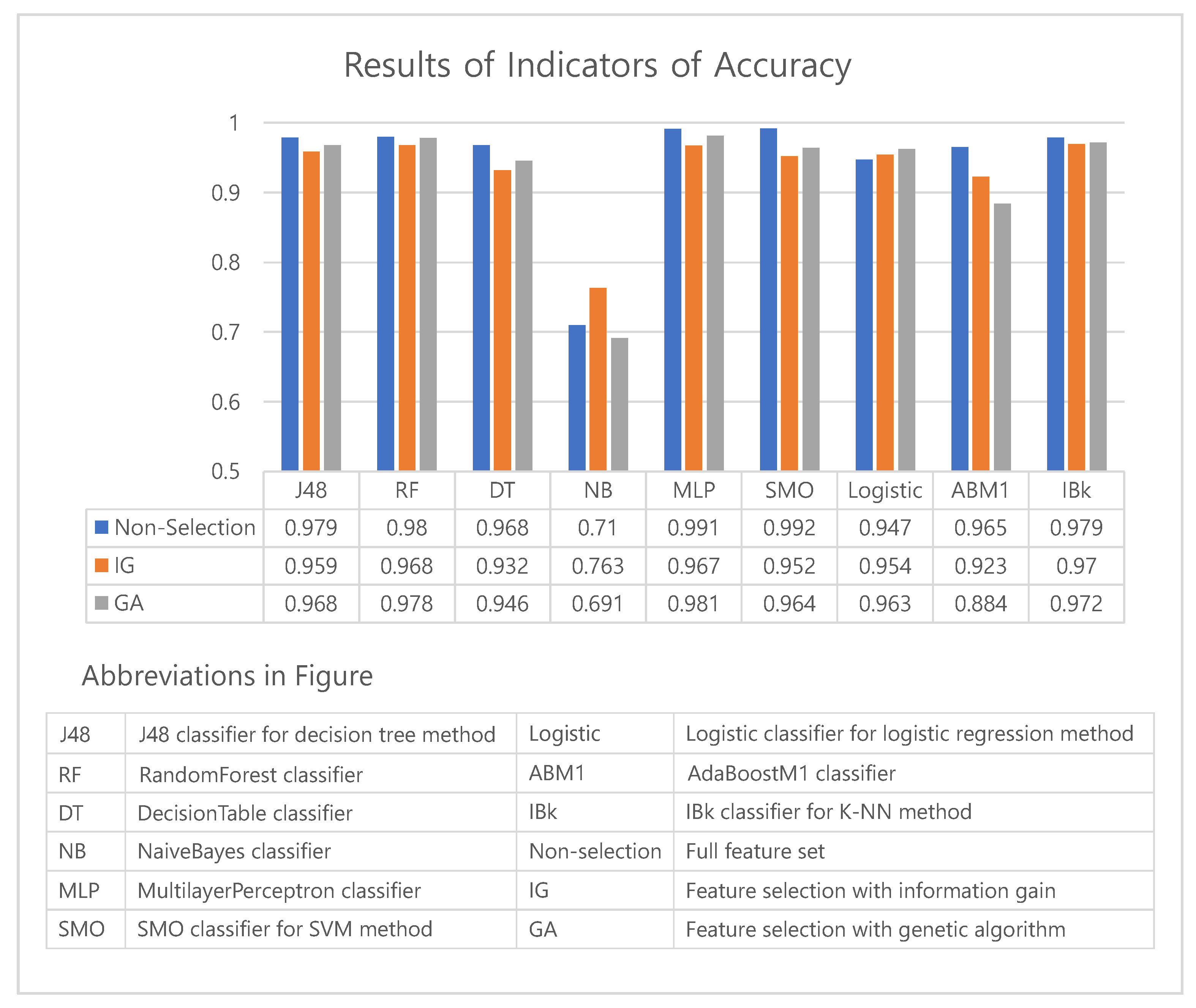
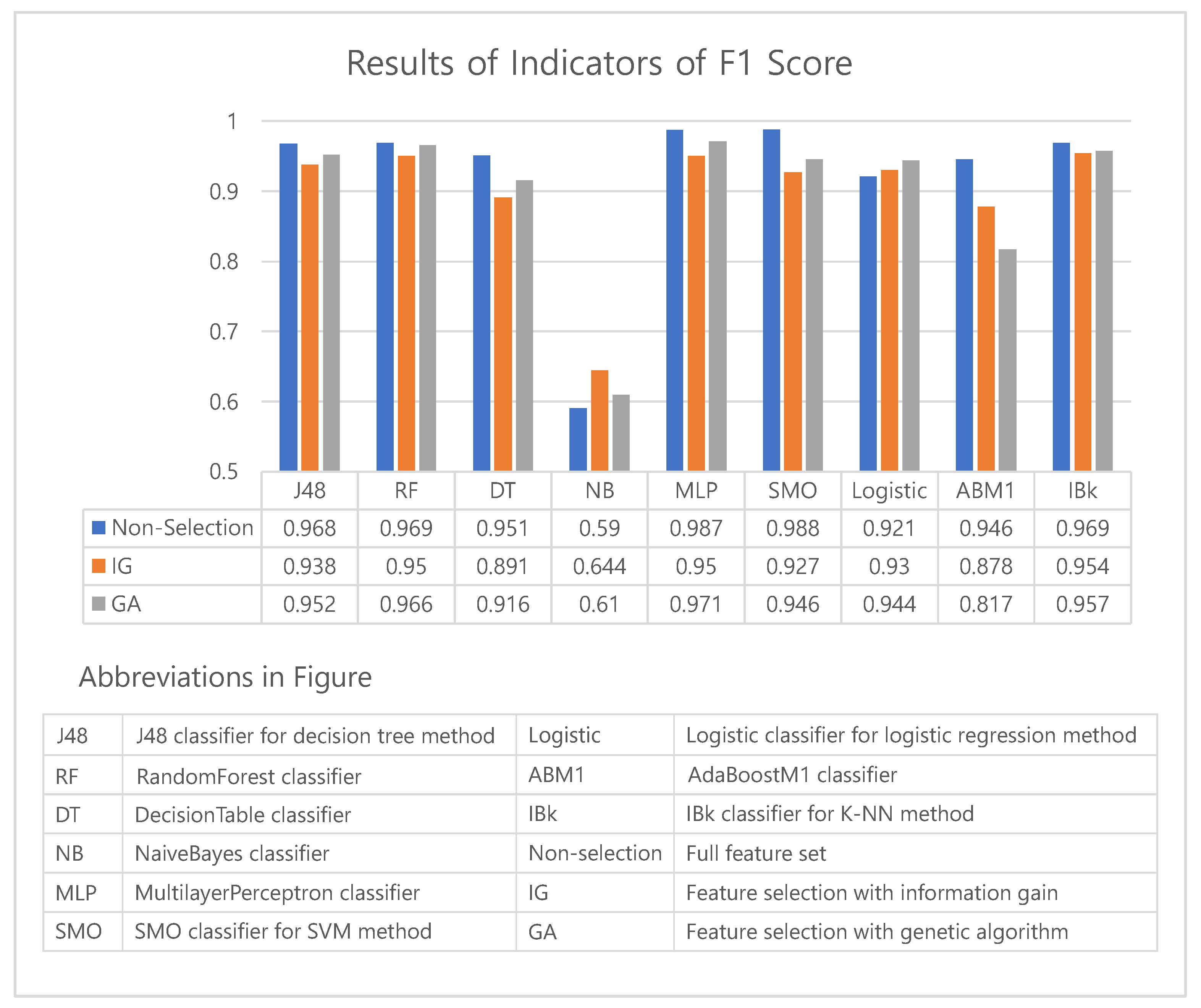
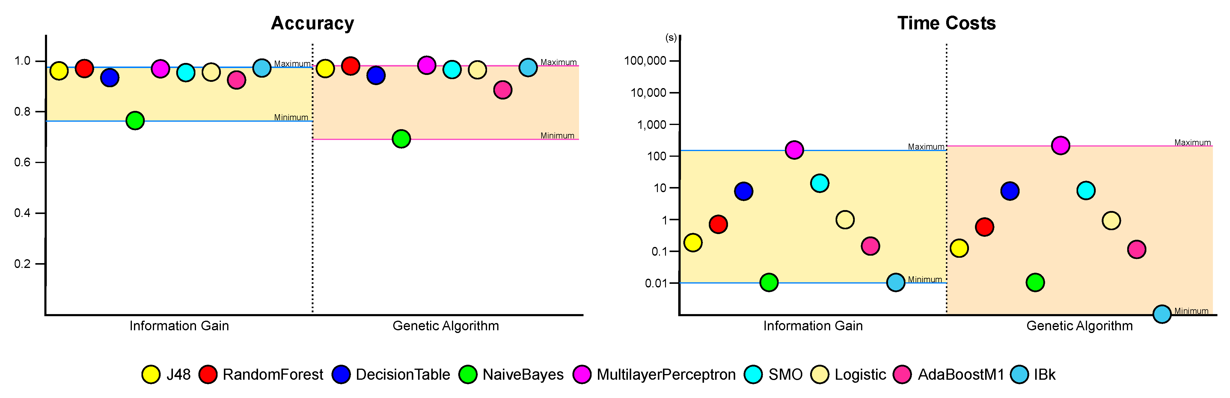
5.1. Accuracy/F1 Score Performance by Algorithm

The accuracy/F1 score results of the experiment described in Section 4 are summarized in

Table 4. Accuracy/F1 score performance results using the various feature selection methods.

Algorithm	Non-Selection		Information Gain		Genetic Algorithm
	Acc.	F1 Score	Acc.	F1 Score	Acc.	F1 Score
J48	0.979	0.968	0.959	0.938	0.968	0.952
RandomForest	0.98	0.969	0.968	0.95	0.978	0.966
DecisionTable	0.968	0.951	0.932	0.891	0.946	0.916
NaiveBayes	0.71	0.59	0.763	0.644	0.691	0.61
MultilayerPerceptron	0.991	0.987	0.967	0.95	0.981	0.971
SMO	0.992	0.988	0.952	0.927	0.964	0.946
Logistic	0.947	0.921	0.954	0.93	0.963	0.944
AdaBoostM1	0.965	0.946	0.923	0.878	0.884	0.817
IBk	0.979	0.969	0.97	0.954	0.972	0.957

. Table 4 shows the classification performances of three methods—classification without feature selection, i.e., non-selection (using full feature set), classification with feature selection by information gain, and classification with feature selection by genetic algorithm.

The experimental results show that the best algorithm for detecting malicious applications varies based on the method of feature selection—SMO for non-selection, IBk for information gain, and MultilayerPerceptron for a genetic algorithm. By contrast, the performance of NaiveBayes’s was shown to be the lowest for all three cases.

Based on the results shown in Table 4, to check the performance of the feature selection algorithm, we made charts to compare the accuracy and F1 score obtained by each method of feature selection. Figure 5 and Figure 6 show graphs of the accuracy and F1 score indicator.

The performance of method without a feature selection(non-selection) generally outperformed the one with a feature selection(IG, GA). However, non-selection results show small differences of less than 0.04 from those of IG and GA for all machine learning algorithms except the AdaBoostM1 (see Figure 5). This result can be analyzed that a feature selection may eliminate over a thousand features, however the degradation of performance is only 4%p. In particular, the degradation of performance of GA was only 3%p (excluding AdaBoostM1). Moreover, the logistic algorithm achieved an increase in accuracy when the feature selection was applied. As shown in Figure 6, we can confirm that the F1 scores also exhibit similar results with those of accuracy. The F1 scores of the NaiveBayes algorithm with a feature selection(IG, GA) was higher than the method without a feature selection(non-selection).

We conducted a t-test to compare the accuracy of the non-selection and genetic algorithms. The results have a significance level of $7.5\times {10}^{-2}$; that is, the performance of non-selection was significantly similar to that of the genetic algorithm. We also conducted a t-test to compare the F1 score. The result has a significance level of $1.5\times {10}^{-1}$, which also shows that the performance was significantly similar to that of the genetic algorithm.

Comparing the feature selection performance of the genetic algorithm to that of information gain, we can confirm that all indicators of the genetic algorithms are superior except for the results of NaiveBayes, by which the information gain achieved a better performance over a non-selection and AdaBoostM1. Although it is not easy to generalize the result because it was impossible to conduct experiments on all algorithms, we can confirm that selecting a genetic algorithm can yield better results than information gain.

5.2. Time Cost for Model Building

The accuracy and F1 scores show that it is advantageous not to proceed with feature selection. However, the machine learning process should also consider the time required to build a model. Therefore, it is also necessary to compare time cost for model building. Machine learning with all features is not always beneficial because it requires much more time to learn many different features’ information.

Table 5. The time cost for building a model for each algorithm.

Algorithm	Time Costs (s)
	Non-Selection	Information Gain	Genetic Algorithm
J48	3.92	0.18	0.12
RandomForest	3.32	0.68	0.56
DecisionTable	100.85	7.48	7.63
NaiveBayes	0.05	0.01	0.01
MultilayerPerceptron	31705.55	150.19	207.93
SMO	11.18	13.44	7.93
Logistic	13.56	0.95	0.89
AdaBoostM1	2.74	0.14	0.11
IBk	0	0.01	0

shows how long it took to build a model for each algorithm.

Other previous works that conducted experiments on malware detection using feature selection similar to this study, such as researches by A. Firdaus et al. [12] and A. Fatima et al. [13], did not mention the time required for feature selection. However, the time used for the feature selection by a genetic algorithm is also the important indicator which should be considered by developers. GA-based feature selection in this study took approximately 54,000 s, about 15 h, with c2-standard-8 virtual machine instance provided by Google Cloud Platform Compute Engine. This is a long time compared to the training time; however, feature selection proceeds not often in general, and it is done only once or performed only when upgrading applications or services. In addition, the feature selection only needs to be performed once for different machine learning models. So about 15 h of feature selection process is available in practice.

Table 5 summarizes that it takes more time to learn the data that have not been selected. In particular, with certain exceptions, datasets that have been selected through genetic algorithms have an advantage over data that have not been selected. Furthermore, except for the result of DecisionTable and MultilayerPerceptron, comparing the two feature selection methods also shows that the genetic algorithm takes less time.

By contrast, as shown in Figure 5 and Figure 6, the performance of the genetic algorithm was better, which means that a genetic algorithm is superior to most algorithms in terms of time or evaluation thereby increasing the expectations of achieving better results.

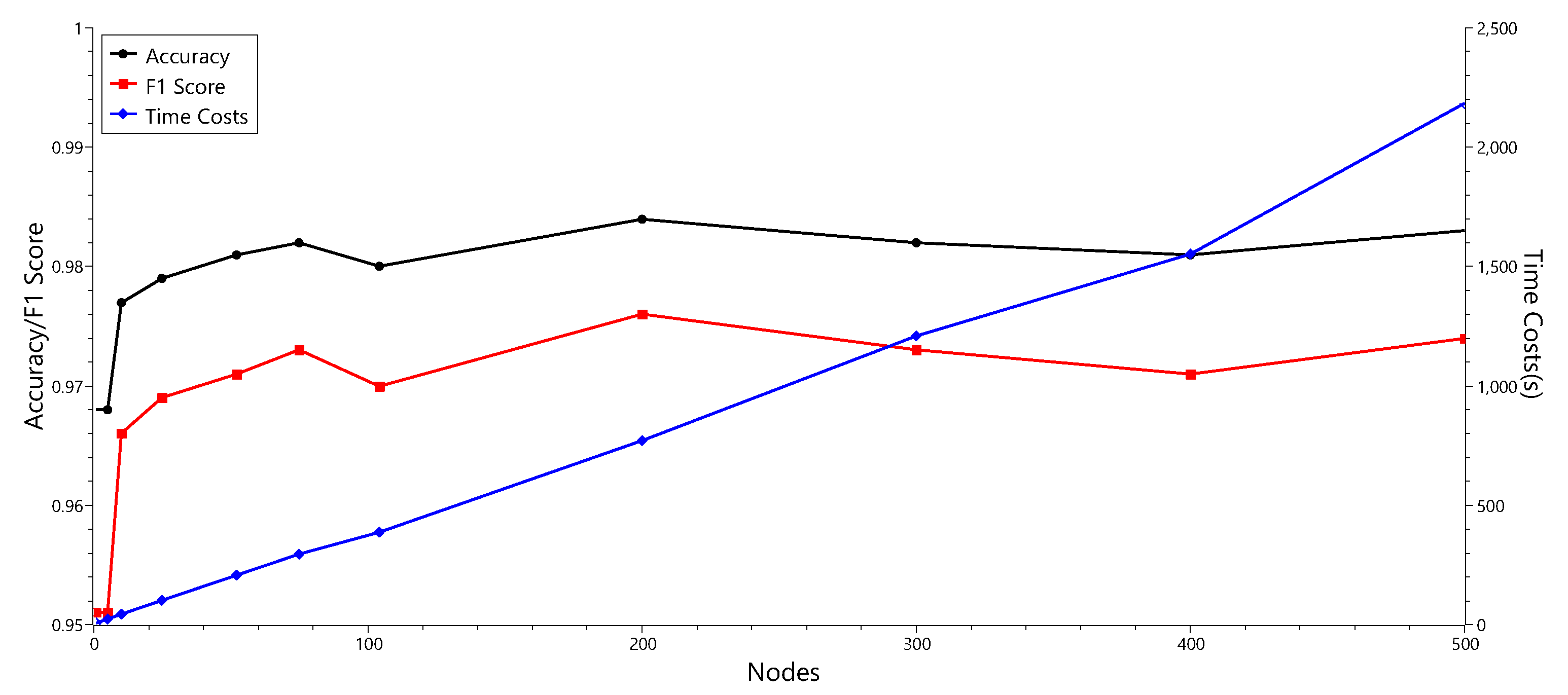
5.3. Hyperpatameter Optimization

The experimental results in the above sections, it was shown that genetic algorithm is a competitive method compared to other feature selection methods. However, there is still a possibility to improve the performances of the machine learning methods. To investigate how much of the performance of the proposed method can be improved, hyperperparameter optimization was applied on the MultilayerPerceptron classifier, which showed the best performance among the machine learning methods used in this study.

MultilayerPerceptron is a classifier provided by WEKA that classifies data through establishing a multilayer neural network. This classifier basically has as many input layer nodes as the number of features, and it has as many output layer nodes as the number of classes. The hidden layer can be set up freely. We tried to build an optimal neural network by adjusting the number of nodes of hidden layer.

The MultilayerPerceptron classifier used in the above experiment had one intermediate layer, and the number of nodes in the intermediate layer was determined by the following formula:

$$\lfloor \frac{attribute+class}{2}\rfloor$$

(6)

In this experiment, there are 102 attributes and 2 classes in the dataset. Thus, there are 52 nodes in hidden layer. We compared the performance of classifiers by changing the number of nodes. The results are summarized in

Table 6. The hyperparameter optimization result for a single hidden layer.

# Nodes	Accuracy	F1 Score	Time Costs (s)
1	0.968	0.951	6.54
5	0.968	0.951	24.24
10	0.977	0.966	43.71
25	0.979	0.969	101
52	0.981	0.971	207.93
75	0.982	0.973	296.95
104	0.98	0.97	387.1
200	0.984	0.976	771.83
300	0.982	0.973	1208.84
400	0.981	0.971	1553.27
500	0.983	0.974	2182.71

and Figure 7.

As shown in Table 6 and Figure 7, the classifier showed the best performance when the hidden layer had 200 nodes. With 200 nodes, the accuracy of the classifier was 0.984, which is a better result than that of previous experiment with 52 nodes, 0.981. By adjusting the parameter values of the MultilayerPerceptron classifier, we could obtain the performance improvement. However, we also observed that increasing the number of nodes in the hidden layer did not necessarily improve the performance. In addition, as the number of nodes increased, the time cost also increased. It is necessary to find an appropriate parameter that can balance performance improvement and time consumption.

To find such a parameter, we also conducted an experiment with double hidden layers. We inserted a new hidden layer with multiple nodes into the existing neural network. The results are summarized in

Table 7. The hyperparameter optimization result for double hidden layers.

Location of New Layer	# Nodes	Accuracy	F1 Score	Time Costs (s)
Before existing layer	1	0.968	0.951	17.88
	25	0.984	0.976	154.59
	52	0.982	0.972	332.12
	104	0.982	0.972	602.83
After existing layer	1	0.982	0.972	162.01
	25	0.981	0.971	243.97
	52	0.982	0.972	332.12
	104	0.98	0.97	530.98

and Figure 8.

Through Table 7 and Figure 8, we can observe that adding a new hidden layer to the neural network can also improve the performance of the classifier. In addition, the best case in this experiment showed the same accuracy as the best MultilayerPerceptron with 200 nodes in a single hidden layer presented in Table 6, while having less time cost than the case before optimization. This means that, adjusting the number of nodes in double hidden layers can be more efficient than that in a single hidden layer.

Through the experiment, we could observe that the performance could be improved by properly manipulating the parameter of the classifier. Through this hyperparameter optimization experiments, we could find the improved parameter combination, which showed the increased accuracy while having the reduced time cost.

5.4. Total Results

In summary, we can conclude that using data without feature selection is the best choice in terms of the evaluation metrics. However, considering the time required, it is better to proceed with feature selection through genetic algorithms, with which we can expect better results than applying information gain. These results can be visualized as Figure 9 and Figure 10.

The results suggest that although feature selection through the genetic algorithm did not result in a performance improvement, applying genetic algorithm can achieve a significant performance as a learning model with much less time and can be superior to a conventional feature selection. It also shows that the performance of machine learning with feature selection based on genetic algorithm can be increased through the result of hyperparameter optimization experiment. In addition, the result from this study is not far behind even when compared to the results of other existing studies.

Table 8. Comparison with previous work.

Reference	Dataset	Set Size	Feature	Feature Selection Method	Classifier	Accuracy	F1 Score
[7]	Drebin	5560	assembly, API calls	none	Random Forest	0.9433	0.94
[10]	VirusShare, APKPure	6000	permission	RFFS+ Acc2+M2	Random Forest	undetermined	0.952
[12]	Drebin, Play store	6105	permission, code-based, directory path	Genetic Selection	Functional Tree (FT)	0.95	0.972
[13]	undetermined	40,000	app component, permission	Genetic Algorithm	SVM	0.95	0.95
[14]	AMGP, Play store	1740	permission	Genetic Algorithm	SVM	0.985	0.981
The best result in this study	Andro-AutoPsy	7500	permission, API method	Genetic Algorithm	MultilayerPerceptron	0.984	0.976

summarized a comparison with previous works. There was only one result to show better performance than ours, the work by [14], and this work used also genetic algorithm-based feature selection. Although Table 8 shows that our method did not produce the best result among the compared other studies, the results also demonstrate the effectiveness of feature selection based on genetic algorithm in Android malware detection.

6. Conclusions

Detecting Android malware in a quick and accurate manner is essential for Android OS users. To solve this problem, many studies have introduced machine learning for the detection of malicious applications, and feature selection has also been employed to speed up the process. In this study, experiments were conducted to select permission and API method information features to apply machine learning based on existing research, and the results indicate that genetic algorithm-based feature selection was also useful compared to a commonly applied information gain. Although the feature selection performance using the genetic algorithm was reduced less than 3%p in general, it also has an advantage over non-selection because it drastically reduces the model’s building time.

The ultimate goal of machine learning is to be able to supply time and space budgets to machine-learning systems in addition to accuracy requirements, with the system finding an operating point that allows such requirements to be realized [56]. Considering this, the experiment results indicate that using genetic algorithms for Android malware detection is also useful compared to other approaches. The experiment also shows that it may be helpful to proceed with feature selection using a genetic algorithm, although the feature selection was applied on a dataset with more than a thousand features.

However, further studies are required to resolve the following issues. In this study, static features were determined using the permission and API method information. As this cannot prove whether feature selection using genetic algorithms is helpful when selecting features using other static and dynamic elements, further discussion of this problem is required. In addition, because this dataset consists of applications collected from January 2013 to April 2014, the results of this study may not be evaluated appropriately in current Android applications owing to the many changes from the current environment during the year 2021. It is necessary to conduct a validation using a dataset consisting of recently released applications.

Although further research and discussion are needed, this study confirmed that genetic algorithms can help machine learning for Android malware detection. If further research results are available in the future, we will note genetic algorithms as a solution for malware detection to achieve higher accuracy with lesser time costs.

References

1. Topgül, O.; Tatlı, E. The Past and Future of Mobile Malwares. In The 7th International Conference on Information Security and Cryptology; Springer: Berlin, German, 2014; pp. 1–7. [Google Scholar]
2. Chebyshev, V. Mobile Malware Evolution 2020. 1 March 2021. Available online: https://securelist.com/mobile-malware-evolution-2020/101029/ (accessed on 7 May 2021).
3. StatCounter. Mobile Operating System Market Share Worldwide. May 2021. Available online: https://gs.statcounter.com/os-market-share/mobile/worldwide (accessed on 10 June 2021).
4. Sawle, P.D.; Gadicha, A. Analysis of malware detection techniques in android. Int. J. Comput. Sci. Mob. Comput. 2014, 3, 176–182. [Google Scholar]
5. Liu, K.; Xu, S.; Xu, G.; Zhang, M.; Sun, D.; Liu, H. A review of android malware detection approaches based on machine learning. IEEE Access 2020, 8, 124579–124607. [Google Scholar] [CrossRef]
6. Wang, Z.; Liu, Q.; Chi, Y. Review of android malware detection based on deep learning. IEEE Access 2020, 8, 181102–181126. [Google Scholar] [CrossRef]
7. Rana, M.S.; Gudla, C.; Sung, A.H. Evaluating machine learning models for Android malware detection: A comparison study. In Proceedings of the 2018 VII International Conference on Network, Communication and Computing, Taipei City, Taiwan, 14–16 December 2018; pp. 17–21. [Google Scholar]
8. Ahmadi, M.; Sotgiu, A.; Giacinto, G. Intelliav: Toward the feasibility of building intelligent anti-malware on android devices. In Cross-Domain Conference for Machine Learning and Knowledge Extraction; Springer: Cham, Switzerland, 2017; pp. 137–154. [Google Scholar]
9. Mahindru, A.; Sangal, A. MLDroid—Framework for Android malware detection using machine learning techniques. Neural Comput. Appl. 2021, 33, 5183–5240. [Google Scholar] [CrossRef]
10. Şahin, D.Ö.; Kural, O.E.; Akleylek, S.; Kılıç, E. A novel Android malware detection system: Adaption of filter-based feature selection methods. J. Ambient. Intell. Humaniz. Comput. 2021, 15, 1–15. [Google Scholar]
11. Lei, S. A Feature Selection Method Based on Information Gain and Genetic Algorithm. In Proceedings of the 2012 International Conference on Computer Science and Electronics Engineering, Hangzhou, China, 23–25 March 2012; Volume 2, pp. 355–358. [Google Scholar]
12. Firdaus, A.; Anuar, N.B.; Karim, A.; Ab Razak, M.F. Discovering optimal features using static analysis and a genetic search based method for Android malware detection. Front. Inf. Technol. Electron. Eng. 2018, 19, 712–736. [Google Scholar]
13. Fatima, A.; Maurya, R.; Dutta, M.K.; Burget, R.; Masek, J. Android malware detection using genetic algorithm based optimized feature selection and machine learning. In Proceedings of the 2019 42nd International Conference on Telecommunications and Signal Processing (TSP), Budapest, Hungary, 1–3 July 2019; pp. 220–223. [Google Scholar]
14. Yildiz, O.; Doğru, I.A. Permission-based android malware detection system using feature selection with genetic algorithm. Int. J. Softw. Eng. Knowl. Eng. 2019, 29, 245–262. [Google Scholar] [CrossRef]
15. Meimandi, A.; Seyfari, Y.; Lotfi, S. Android malware detection using feature selection with hybrid genetic algorithm and simulated annealing. In Proceedings of the 2020 IEEE 5th Conference on Technology In Electrical and Computer Engineering (ETECH 2020) Information and Communication Technology (ICT), Tehran, Iran, 22 October 2020. [Google Scholar]
16. Wang, J.; Jing, Q.; Gao, J.; Qiu, X. SEdroid: A robust Android malware detector using selective ensemble learning. In Proceedings of the 2020 IEEE Wireless Communications and Networking Conference (WCNC), Seoul, Korea, 25–28 May 2020; pp. 1–5. [Google Scholar]
17. Wang, L.; Gao, Y.; Gao, S.; Yong, X. A New Feature Selection Method Based on a Self-Variant Genetic Algorithm Applied to Android Malware Detection. Symmetry 2021, 13, 1290. [Google Scholar]
18. Ratazzi, E.P. Understanding and improving security of the Android operating system. Ph.D. Thesis, Syracuse University, Syracuse, NY, USA, 2016. [Google Scholar]
19. Aswini, A.M.; Vinod, P. Droid permission miner: Mining prominent permissions for Android malware analysis. In Proceedings of the Fifth International Conference on the Applications of Digital Information and Web Technologies (ICADIWT 2014), Chennai, India, 17–19 February 2014; pp. 81–86. [Google Scholar]
20. Yen, Y.S.; Sun, H.M. An Android mutation malware detection based on deep learning using visualization of importance from codes. Microelectron. Reliab. 2019, 93, 109–114. [Google Scholar]
21. Lim, K.; Kim, N.Y.; Jeong, Y.; Cho, S.j.; Han, S.; Park, M. Protecting Android Applications with Multiple DEX Files Against Static Reverse Engineering Attacks. Intell. Autom. Soft Comput. 2019, 25, 143–154. [Google Scholar]
22. Bhatt, M.S.; Patel, H.; Kariya, S. A survey permission based mobile malware detection. Int. J. Comput. Technol. Appl. 2015, 6, 852–856. [Google Scholar]
23. Emanuelsson, P.; Nilsson, U. A comparative study of industrial static analysis tools. Electron. Notes Theor. Comput. Sci. 2008, 217, 5–21. [Google Scholar] [CrossRef] [Green Version]
24. Amro, B. Malware Detection Techniques for Mobile Devices. Int. J. Mob. Netw. Commun. Telemat. 2017, 7, 1–10. [Google Scholar] [CrossRef]
25. Ball, T. The concept of dynamic analysis. In Software Engineering—ESEC/FSE’99; Springer: Berlin/Heidelberg, Germany, 1999; pp. 216–234. [Google Scholar]
26. Wong, M.Y.; Lie, D. IntelliDroid: A Targeted Input Generator for the Dynamic Analysis of Android Malware. In Proceedings of the Annual Symposium on Network and Distributed System Security (NDSS), San Diego, CA, USA, 21–24 February 2016. [Google Scholar]
27. Guyon, I.; Elisseeff, A. An introduction to variable and feature selection. J. Mach. Learn. Res. 2003, 3, 1157–1182. [Google Scholar]
28. Li, J.; Cheng, K.; Wang, S.; Morstatter, F.; Trevino, R.P.; Tang, J.; Liu, H. Feature selection: A data perspective. ACM Comput. Surv. (CSUR) 2017, 50, 1–45. [Google Scholar] [CrossRef] [Green Version]
29. Hsu, H.H.; Hsieh, C.W.; Lu, M.D. Hybrid feature selection by combining filters and wrappers. Expert Syst. Appl. 2011, 38, 8144–8150. [Google Scholar] [CrossRef]
30. Kohavi, R.; John, G.H. Wrappers for feature subset selection. Artif. Intell. 1997, 97, 273–324. [Google Scholar] [CrossRef] [Green Version]
31. Lee, S.J.; Moon, H.J.; Kim, D.J.; Yoon, Y. Genetic algorithm-based feature selection for depression scale prediction. In Proceedings of the ACM GECCO Conference, Prague, Czech Republic, 13–17 July 2019; pp. 65–66. [Google Scholar]
32. Mitchell, M. An Introduction to Genetic Algorithms; MIT Press: Cambridge, MA, USA, 1998. [Google Scholar]
33. Lambora, A.; Gupta, K.; Chopra, K. Genetic algorithm-A literature review. In Proceedings of the 2019 International Conference on Machine Learning, Big Data, Cloud and Parallel Computing (COMITCon), Faridabad, India, 14–16 February 2019; pp. 380–384. [Google Scholar]
34. Panchal, G.; Panchal, D. Solving NP hard problems using genetic algorithm. Transportation 2015, 106, 6-2. [Google Scholar]
35. Montazeri, M.; Montazeri, M.; Naji, H.R.; Faraahi, A. A novel memetic feature selection algorithm. In Proceedings of the 5th Conference on Information and Knowledge Technology, Shiraz, Iran, 28–30 May 2013; pp. 295–300. [Google Scholar]
36. Whitley, D. A genetic algorithm tutorial. Stat. Comput. 1994, 4, 65–85. [Google Scholar] [CrossRef]
37. Alpaydin, E. Introduction to Machine Learning, 2nd ed.; MIT Press: Cambridge, MA, USA, 2009. [Google Scholar]
38. Mitchell, T.M. Machine Learning; McGraw-Hill: New York, NY, USA, 1997. [Google Scholar]
39. Su, J.; Zhang, H. A fast decision tree learning algorithm. In Proceedings of the America Association for Artificial Intelligence, Boston, MA, USA, 16–20 July 2006; Volume 6, pp. 500–505. [Google Scholar]
40. Breiman, L. Random forests. Mach. Learn. 2001, 45, 5–32. [Google Scholar] [CrossRef] [Green Version]
41. Witt, G. Writing Effective Business Rules; Morgan Kaufmannr: Burlington, MA, USA, 2012. [Google Scholar]
42. Kalmegh, S.R. Comparative analysis of the weka classifiers rules conjunctive rule & decision table on indian news dataset by using different test mode. Int. J. Eng. Sci. Invent. (IJESI) 2018, 7, 1–9. [Google Scholar]
43. John, G.H.; Langley, P. Estimating continuous distributions in Bayesian classifiers. In Proceedings of the 11th Conference on Uncertainty in Artificial Intelligence, Montreal, QC, Canada, 18 August 1995; pp. 338–345. [Google Scholar]
44. Abirami, S.; Chitra, P. Energy-efficient edge based real-time healthcare support system. In Advances in Computers; Elsevier: Amsterdam, The Netherlands, 2020; Volume 117, pp. 339–368. [Google Scholar]
45. Montúfar, G.; Pascanu, R.; Cho, K.; Bengio, Y. On the number of linear regions of deep neural networks. In Proceedings of the NIPS’14: Proceedings of the 27th International Conference on Neural Information Processing Systems, Montreal, QC, Canada, 8 December 2014; Volume 27. [Google Scholar]
46. Cortes, C.; Vapnik, V. Support-vector networks. Mach. Learn. 1995, 20, 273–297. [Google Scholar] [CrossRef]
47. Fatah, K.; Mahmood, F.R. Parameter Estimation for Binary Logistic Regression Using Different Iterative Methods. J. Zankoy Sulaimani Part A 2017, 19, 175–184. [Google Scholar]
48. Freund, Y.; Schapire, R.E. A Decision-Theoretic Generalization of On-Line Learning and an Application to Boosting. J. Comput. Syst. Sci. 1997, 55, 119–139. [Google Scholar]
49. Freund, Y.; Schapire, R. A Short Introduction to Boosting. J. Jpn. Soc. Artif. Intell. 1999, 14, 771–780. [Google Scholar]
50. Kuang, Q.; Zhao, L. A Practical GPU Based KNN Algorithm. In Proceedings of the Second Symposium International Computer Science and Computational Technology(ISCSCT’09), Huangshan, China, 26 December 2009. [Google Scholar]
51. Androguard. Available online: https://github.com/androguard/androguard (accessed on 8 May 2021).
52. Eibe, F.; Hall, M.A.; Witten, I.H. The WEKA Workbench. Online Appendix for Data Mining: Practical Machine Learning Tools and Techniques; Morgan Kaufmann: Burlington, MA, USA, 2016. [Google Scholar]
53. Jang, J.W.; Kang, H.; Woo, J.; Mohaisen, A.; Kim, H.K. Andro-AutoPsy: Anti-malware system based on similarity matching of malware and malware creator-centric information. Digit. Investig. 2015, 14, 17–35. [Google Scholar] [CrossRef]
54. Syswerda, G. Uniform Crossover in Genetic Algorithms. In Proceedings of the 3rd International Conference on Genetic Algorithms, Fairfax, VA, USA, 4 June 1989. [Google Scholar]
55. Kim, T.K. T test as a parametric statistic. Korean J. Anesthesiol. 2015, 68, 540. [Google Scholar] [CrossRef] [Green Version]
56. Jordan, M.I.; Mitchell, T.M. Machine learning: Trends, perspectives, and prospects. Science 2015, 349, 255–260. [Google Scholar] [CrossRef]
Figure 1. The main structure of an APK file [18].
Mathematics 09 02813 g001
Figure 2. Simplified flowchart of the genetic algorithm’s progression.
Mathematics 09 02813 g002
Figure 3. Flowchart of experiment progression.
Mathematics 09 02813 g003
Figure 4. The performance of the genetic algorithm in Section 4.3 according to the number of generations.
Mathematics 09 02813 g004
Figure 5. A graph comparing accuracy among feature selection methods.
Mathematics 09 02813 g005
Figure 6. A graph comparing F1 scores among feature selection methods.
Mathematics 09 02813 g006
Figure 7. Schematization of a hyperparameter optimization result for a single hidden layer.
Mathematics 09 02813 g007
Figure 8. Schematization for the hyperparameter optimization result for double hidden layers.
Mathematics 09 02813 g008
Figure 9. A comparison of machine learning performances between non-selection and genetic algorithm-based feature selection.
Mathematics 09 02813 g009
Figure 10. A comparison of machine learning performances between information gain-based and genetic algorithm-based feature selection.
Mathematics 09 02813 g010