Search Graph Magnification in Rapid Mixing of Markov Chains Associated with the Local Search-Based Metaheuristics

Abstract

The structural property of the search graph plays an important role in the success of local search-based metaheuristic algorithms. Magnification is one of the structural properties of the search graph. This study builds the relationship between the magnification of a search graph and the mixing time of Markov Chain (MC) induced by the local search-based metaheuristics on that search space. The result shows that the ergodic reversible Markov chain induced by the local search-based metaheuristics is inversely proportional to magnification. This result indicates that it is desirable to use a search space with large magnification for the optimization problem in hand rather than using any search spaces. The performance of local search-based metaheuristics may be good on such search spaces since the mixing time of the underlying Markov chain is inversely proportional to the magnification of search space. Using these relations, this work shows that MC induced by the Metropolis Algorithm (MA) mixes rapidly if the search graph has a large magnification. This indicates that for any combinatorial optimization problem, the Markov chains associated with the MA mix rapidly i.e., in polynomial time if the underlying search graph has large magnification. The usefulness of the obtained results is illustrated using the $0/1$-Knapsack Problem, which is a well-studied combinatorial optimization problem in the literature and is NP-Complete. Using the theoretical results obtained, this work shows that Markov Chains (MCs) associated with the local search-based metaheuristics like random walk and MA for $0/1$-Knapsack Problem mixes rapidly.

1. Introduction

Most of the combinatorial optimization problems in the real world have high computational complexity, which implies there are no known polynomial time algorithms that exist for such optimization problems. For example, there is the Traveling Salesman problem [1], Covering Salesman problem [2], $0/1$-Knapsack Problem [3], Knapsack Problem with Forfeits [4], multiple demand multiple-choice multidimensional Knapsack Problem [5], Longest path problem [6], Scheduling problem [7], Truck Scheduling [8,9], and Flexible Flowshop Scheduling [10] etc. There is no good polynomial time approximation algorithm for such problems (for example, Shortest Vector Problem [11]). Hence, a practitioner or researcher makes use of metaheuristics such as Evolutionary Algorithm (EA) [12], Metropolis Algorithm (MA) [13], Simulated annealing (SA) [14], Particle Swarm Optimization (PSO) [15], Ant Colony Optimization (ACO) [16] etc., to get near to the optimum solution for the problem. Performance analysis of metaheuristics are not simple, since it is highly random in nature. MCs are one of the widely used methods to analyze the performance of metaheuristics [17,18,19,20,21,22,23,24,25,26,27,28,29,30].

Metaheuristics are applied successfully to obtain the optimum or near to optimum solution for many optimization problems in the literature [31,32,33,34,35,36,37,38]. To apply metaheuristics for the optimization problem, one should define a search space for the problem. Once the search space is defined, a practitioner can apply different metaheuristics algorithms using that search space and try to locate the desired solution. Local search-based metaheuristics such as SA, MA, random walk [39], iterated local search [40], etc., search the search space locally. This means that local search-based metaheuristics search the neighborhood of the current state and move from one state to another state locally and try to locate near to the optimum solution for the optimization problem. Hence, to apply local search-based metaheuristics, a researcher must define a search space and neighborhood structure for the problem at hand. Therefore, defining an appropriate and good search space plays a crucial role in the success of metaheuristics. Appropriate means that a search space for the problem should contain all the feasible solutions. Good means that the search space that is defined should have good structural properties. The search space should be connected. This will ensure that any local search-based metaheuristic algorithms using this search space may be able to search all the feasible solutions by moving from one feasible solution to another feasible solution. Secondly, an important structural property is called magnification. Magnification of the search graph indicates the number of edges going out from any cut-set in the search graph. Lower bound on magnification implies the minimum number of edges going out from any cut-set in the search graph. Large magnification implies many edges going out from any cut-set in the search graph. This property may be profitably when used by metaheuristic algorithms to avoid getting stuck at local optima and to reach global optima.

This work shows the importance of designing a good search space for the optimization problem. The results obtained indicate that the success of local search-based metaheuristics depend on the structural property of a search space for the problem. A structural property called magnification [41] of the search graph plays an important role in the rapid mixing of MC induced by local search-based metaheuristics. The proposed study shows that magnification is inversely proportional to the mixing time of MC induced by local search-based metaheuristics. Using the established result between the mixing time of MC and magnification, the study further shows that the MC induced by MA mixes rapidly. Note that MA is a widely used local search-based metaheuristic [42]. As per the literature, it is successful in finding a good solution for many optimization problems [11,41,42,43,44,45,46,47,48,49,50]. Further details about MA are discussed in Section 4.

The mixing time of the Markov chain plays an important role in the run time analysis of the metaheuristic algorithms. It gives the convergence speed of MC to the stationary distribution. It quantifies how close the chain is to its stationary distribution. If the Markov chain induced by metaheuristic algorithm has rapid mixing time i.e., in polynomial time, then running the metaheuristic algorithm that amount of time and taking samples may give the desired solution for the combinatorial optimization problem at hand. Theoretical analysis of a metaheuristic algorithm is not an easy task since they are highly probabilistic in nature. Sanyal et al. proved that one of the necessary and sufficient conditions for the success of the Metropolis algorithm is rapid mixing of the Markov chain induced by the algorithm [43]. In the proposed work we prove that if the search graph has large magnification, then the MC induced by MA mixes rapidly i.e., in polynomial time. The major contributions of the proposed work are listed below:

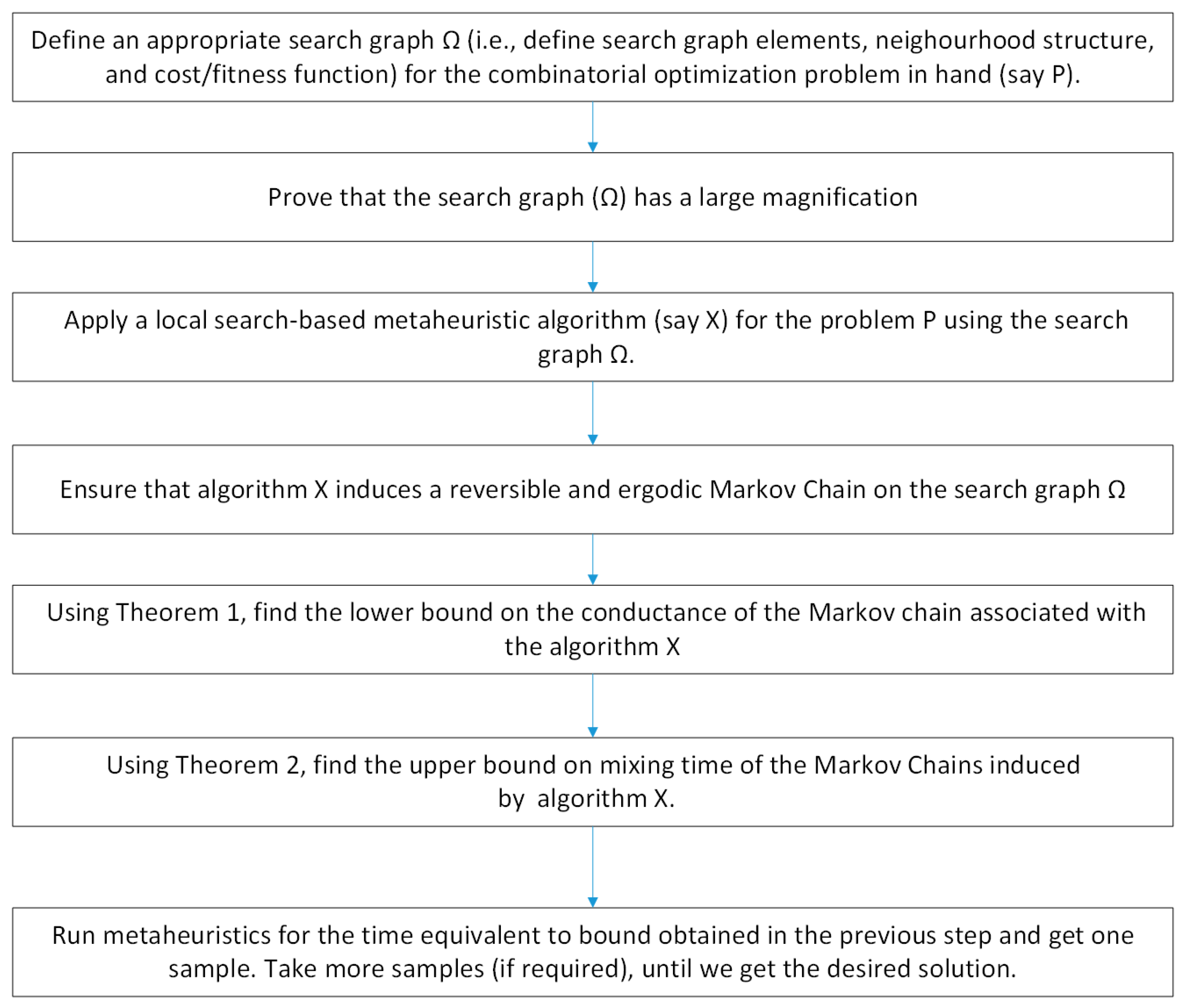
• Establishes the relationship between search graph magnification and conductance of reversible MC induced by local search-based metaheuristics (Refer Theorem 1);
• Establishes the relationship between search graph magnification and mixing time of reversible ergodic MC induced by local search-based metaheuristics (Refer Theorem 2);
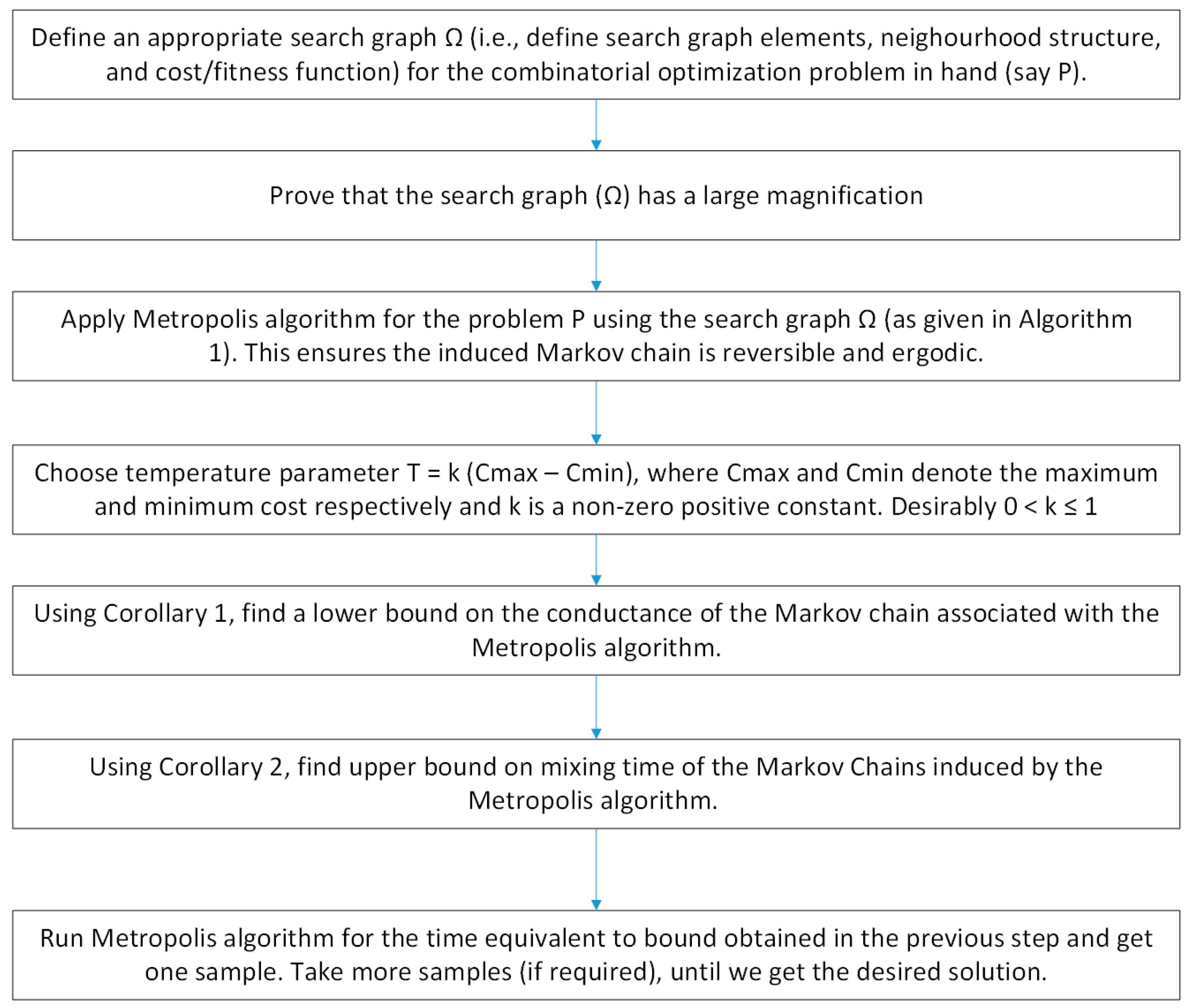
• Proved that if the designed search graph has large magnification, then for a particular choice of temperature parameter, the MC induced by MA mixes rapidly, i.e., in polynomial time (Refer Corollarys 1 and 2);
• Applications of the results obtained are illustrated using $0/1$-Knapsack Problem(Refer Section 5).
  • The search graph for $0/1$-Knapsack Problem has large magnification (Refer Proposition 1);
  • Conductance of MC induced by random walk for $0/1$-Knapsack Problem is large and MC induced by random walk mixes rapidly (Refer Corollary 3);
  • Conductance of MC induced by MA for $0/1$-Knapsack problem is large and MC induced by MA mixes rapidly (Refer Corollary 4).

The paper is organized as follows. The following section discusses basic definition and concepts needed to understand the proposed work. Section 3 establishes the relationship between magnification of search graph and reversible MCs. The relation between magnification and mixing time of the MCs induced by MA is discussed in Section 4. Applications of the theoretical results obtained are illustrated Using $0/1$-Knapsack problem in Section 5 followed by the conclusion.

2. Preliminaries

The search graph (or search space) represents the set of all feasible solutions for any discrete optimization problem. Any metaheuristics such as EA, MA, SA, etc., search this search graph using some heuristics to locate the optimum or near to optimum solution. The search graph has three components:

• Search graph elements: Feasible solutions of the optimization problem;
• Neighborhood structure: How two or more search graph elements are connected i.e., adjacency information;
• Cost or fitness for each element in the search graph.

Based on the problem definition, one has to define the appropriate neighborhood structure and fitness/cost function. For basic definition of MC and its mixing time, refer to the standard textbooks and paper given in the literature [41,48,49,51,52].

Definition 1

(Markov Chain (MC) [41]). A random variable sequence ${\chi }_1,{\chi }_2,{\chi }_3,\dots$ is a MC, if the probability of the future state, given the present sate, is independent of past states. i.e., $Prob({\chi }_t=b|{\chi }_{t-1}=a,\dots ,{\chi }_0=x_0)=Prob({\chi }_t=b|{\chi }_{t-1}=a)$.

The set of all possible values of ${\chi }_i$ is the state space $\Omega$ of the chain. A transition matrix $P={\left(P_{a,b}\right)}_{a,b\in \Omega }$ denotes the transition probability of moving from state a to b.

Next, to define stationary distribution of a MC.

Definition 2

(Stationary Distribution [51,52]). Stationary distribution π is a probability distribution on state space Ω such that $\pi =\pi P$, i.e., ${\sum }_{a\in \Omega }{\pi }_a{P}_{a,b}={\pi }_b$.

Definition 3

(Irreducible MC [41]). Let P denote transition matrix of a MC. A MC with transition matrix P is irreducible If $\forall a,b\in \Omega$, there exists some t such that $P_{a,b}^t>0$ then the MC is aperiodic.

Which implies that the probability of reaching any state to any other state is greater than zero. This implies that the underlying search graph is connected.

Definition 4

(Aperiodic chain [41]). Let P denote the transition matrix of the MC on state space Ω. If $\forall a,bin\Omega$, $\gcd \{t:P_{a,b}^t>0\}=1$, then the MC is aperiodic.

If a chain is aperiodic and irreducible, then it is called a ergodic chain. It is a well-known fact that an ergodic chain has stationary distribution, and it is unique (a fundamental theorem of the MC [52]). Lazy MCs are chains that feel lazy and stay in the same state with probability $\frac{1}{2}$. By choosing self-loop probability $1/2$, one can ensure that MC is lazy. Lazy MCs are aperiodic [52]. An ergodic MC is reversible ${\pi }_a{P}_{a,b}={\pi }_b{P}_{b,a}$, i.e., flow from a to b is the same as flow from b to a [52].

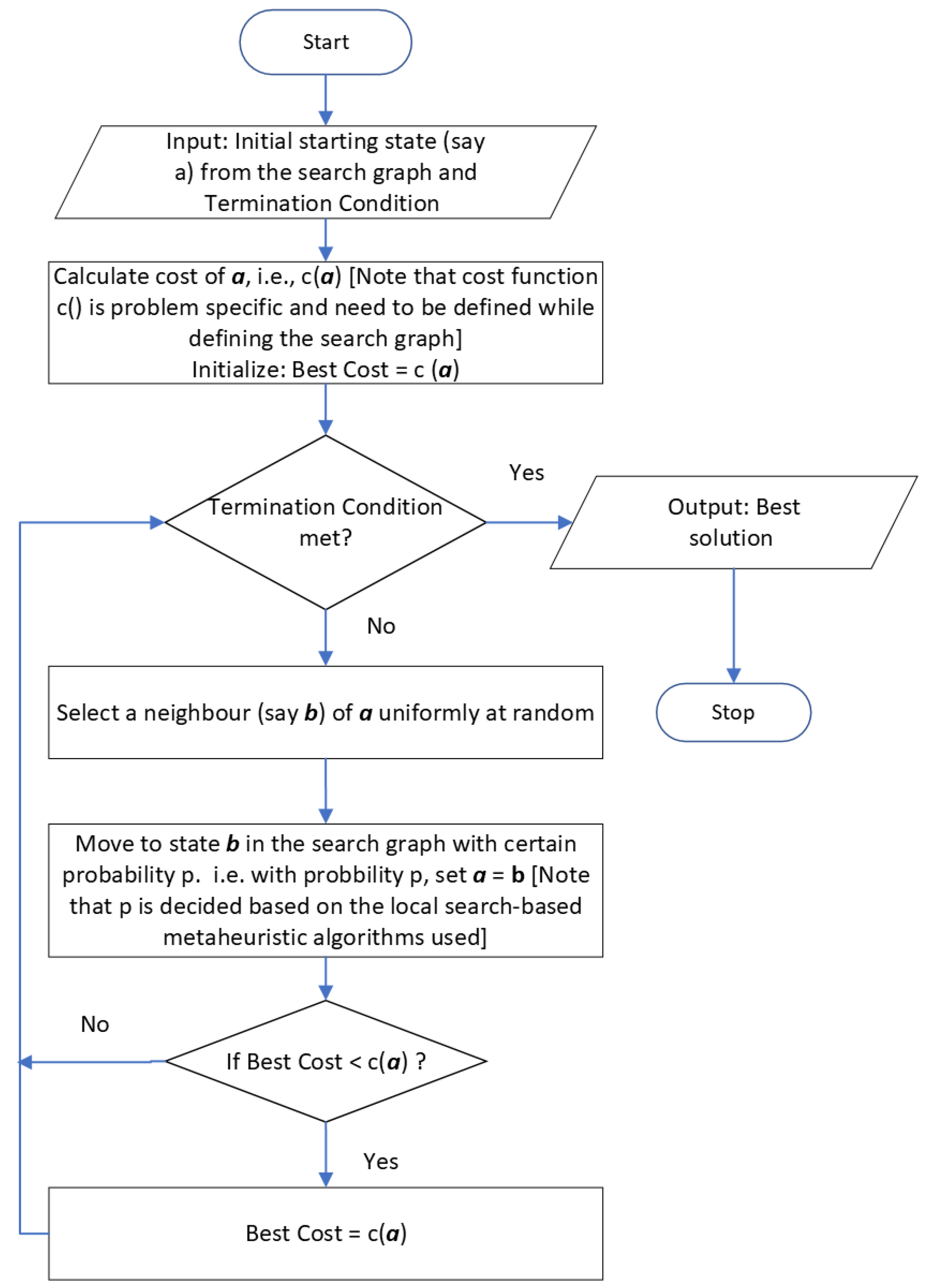
3. Relation between Magnification of Search Graph and Reversible MCs

This section discusses the methods to build relation between magnification of a search graph and mixing time of reversible MCs. Magnification gives a lower bound for the number of arcs (or edges) leaving from any cut set. More formally, it is defined as:

Definition 5

(Magnification (c.f. [41], Proposition 2.11)). Let $\mu (\Omega )$ denote magnification of the search graph Ω and $S\subset \Omega$ and is non empty. Then,

$$\mu (\Omega )=\underset{S}{min}\{\mu \left(S\right):|S|\le |\Omega |/2\},$$

where,

$$\mu \left(S\right)=\frac{\left|\mathcal{E}\right(S,\overline{S}\left)\right|}{\left|S\right|}$$

(1)

and $\mathcal{E}(S,\overline{S})$ denote the number of arcs leaving from S to $\overline{S}$ (where $\overline{S}$ represents the complement of S), respectively.

Now assume that a local search metaheuristic can induce a reversible MC on the search graph $\Omega$. The aim is to establish a relationship between magnification and mixing time of this induced reversible MC. For this, the concept of conductance is needed. Conductance of a MC is defined as:

Definition 6

(Conductance [41]). For any non-empty subset S, Conductance ($\varphi \left(S\right)$ say) is defined as

$$\varphi \left(S\right)=\frac{F_S}{C_S}=\frac{{\sum }_{u\in S,v\in \overline{S}}{P}_{u,v}·{\pi }_u}{{\sum }_{u\in S}{\pi }_u},$$

(2)

where $F_S$ and $C_S$ denote the flow and capacity of set S.

The conductance $\varphi \left(P\right)$ of the chain P (say) is defined as

$$\varphi \left(P\right)=\underset{S:C_S\le \frac{1}{2}}{min}\varphi \left(S\right)$$

(3)

Conductance is a powerful measure which gives conditional probability of the chain getting stuck at any cut set. Large conductance implies large ergodic flow leaving from any cut set. Now to establish the relationship between magnification and conductance.

Theorem 1.

Let $\mu (\Omega )$ and $\varphi \left(P\right)$ denote magnification of search graph Ω and conductance of the reversible ergodic MC with transition matrix P, respectively, then $\varphi \left(P\right)\ge P_{{\{u,v\in N\left(u\right)\}}_{min}}\frac{{\pi }_{min}}{{\pi }_{max}}·\mu (\Omega )$, where $P_{{\{u,v\}}_{min}}$ denote minimum transition probability from u to a neighbor of u say v, $N\left(u\right)$ denotes neighbors of u and ${\pi }_{min}$, ${\pi }_{max}$ denotes minimum and maximum probability in the stationary distribution.

Proof. 

Let $S\subset \Omega$ and $C_S\le \frac{\varphi \left(S\right)}{2}$. Using Definition 6,

$$\begin{array}{cc}\hfill \varphi \left(S\right)& =\frac{{\sum }_{u\in S,v\in \overline{S}}{P}_{u,v}·{\pi }_u}{{\sum }_{u\in S}{\pi }_u}\hfill \\ \hfill & \ge \frac{P_{{\{u,v\in N\left(u\right)\}}_{min}}·{\pi }_{min}·\left|\mathcal{E}(S,\overline{S})\right|}{{\sum }_{u\in S}{\pi }_u}\hfill \\ \hfill & (\mathrm{Sin}\mathrm{ce}\mathrm{there}\mathrm{are}\left|\mathcal{E}\right(S,\overline{S}\left)\right|\mathrm{edges}\mathrm{leaving}\mathrm{from}S\mathrm{to}\overline{S}\hfill \\ \hfill & \mathrm{and}\mathrm{the}\mathrm{chain}\mathrm{is}\mathrm{reversible}.)\hfill \\ \hfill & \ge P_{{\{u,v\in N\left(u\right)\}}_{min}}·\frac{{\pi }_{min}}{{\pi }_{max}}·\frac{\left|\mathcal{E}\right(S,\overline{S}\left)\right|}{\left|S\right|}\hfill \\ \hfill & \ge P_{{\{u,v\in N\left(U\right)\}}_{min}}\frac{{\pi }_{min}}{{\pi }_{max}}·\mu (\Omega )\hfill \end{array}$$

Therefore, $\varphi \left(P\right)\ge P_{{\{u,v\in N\left(u\right)\}}_{min}}\frac{{\pi }_{min}}{{\pi }_{max}}·\mu (\Omega )$. Hence the proof. □

Next is to find bound on mixing time of reversible ergodic MC using magnification. Time taken by a MC to reach its stationary distribution from any starting distribution is called mixing time of the chain. It is important to know how fast or quickly a chain reaches close or near to the stationary distribution. The following lemma gives upper bound for mixing time using the concept of conductance.

Lemma 1

(Mixing Time Lemma [41], Corollary 2.8). For any reversible ergodic MC

$$t_{\mathrm{mix}}\left(\epsilon \right)\le \frac{2}{\varphi {\left(P\right)}^2}·\left(ln{\epsilon }^{-1}+ln{\pi }_{min}^{-1}\right)$$

where the notation ${\pi }_{min}$ is used to denote the minimum probability in π (i.e., in stationary distribution) and $t_{\mathrm{mix}}\left(\epsilon \right)$ is used to denote the mixing time of the chain when it is ε close to stationary distribution.

Now to establish relation between magnification and mixing time. The following theorem gives upper bound for mixing time using magnification.

Theorem 2.

The relationship between search graph magnification ($\mu (\Omega )$) and mixing time of reversible ergodic MC ($t_{\mathrm{mix}}\left(\epsilon \right)$) is:

$$t_{\mathrm{mix}}\left(\epsilon \right)\le \frac{4ln{\pi }_{min}^{-1}}{P_{{\{u,v\in N\left(u\right)\}}_{min}}^2·\mu {(\Omega )}^2}·\frac{{\pi }_{max}^2}{{\pi }_{min}^2}$$

(4)

Proof. 

Using Lemma 1:

$$t_{\mathrm{mix}}\left(\epsilon \right)\le \frac{2}{\varphi {\left(P\right)}^2}·\left(ln{\epsilon }^{-1}+ln{\pi }_{min}^{-1}\right)$$

(5)

and by Theorem 1,

$$\varphi \left(P\right)\ge P_{{\{u,v\in N\left(u\right)\}}_{min}}\frac{{\pi }_{min}}{{\pi }_{max}}·\mu (\Omega )$$

(6)

Using Equations (5) and (6):

$$t_{\mathrm{mix}}\left(\epsilon \right)\le \frac{2}{P_{{\{u,v\in N\left(u\right)\}}_{min}}^2·\mu {(\Omega )}^2}·\frac{{\pi }_{max}^2}{{\pi }_{min}^2}·\left(ln{\epsilon }^{-1}+ln{\pi }_{min}^{-1}\right)$$

Now, by choosing $\epsilon ={\pi }_{min}/2$:

$$t_{\mathrm{mix}}\left(\epsilon \right)\le \frac{4ln{\pi }_{min}^{-1}}{P_{{\{u,v\in N\left(u\right)\}}_{min}}^2·\mu {(\Omega )}^2}·\frac{{\pi }_{max}^2}{{\pi }_{min}^2}$$

 □

The above results shows that if the stationary distribution is inverse exponential and ratio between ${\pi }_{min}$ and ${\pi }_{max}$ is polynomial in input size then mixing time of the Markov chain induced by local search-based metaheuristics mixes rapidly, which is in polynomial time. A flowchart representing the general structure of local search-based metaheuristic algorithm is given in Figure 1 and a detailed block diagram explaining how to apply the proposed method for the combinatorial optimization problem is given in Figure 2.

4. Relation between Magnification and Mixing Time of the MCs Induced by MA

MA is a widely used local search-based metaheuristic and is a modified version of SA [14]. In SA, temperature decreases slowly in every iteration, whereas in the MA temperature is a constant in all the iterations. In SA, the algorithms give better results when temperature is tending to zero, whereas in MA, one must find for which value of temperature parameter we get the desired solution. So, even for one value of temperature parameter, if the MA gives a desirable solution, then we are through. MA induces reversible MC on any irreducible state space $\Omega$ with the desired stationary distribution. This is the beauty of this algorithm. Without loss of generality, this section will explain the MA for maximization problem (similar arguments holds for minimization problem also). MA try to locate the optimum and near optimum solution by searching search graph elements using biased random walk (non-uniform). In each iteration, the algorithm selects any one of the neighbors uniformly at random. If the fitness of the selected neighbor is better (i.e., maximum for maximization problem), then it will move to that state, otherwise it will move to that state with smaller probability, which implies the MA moves to the worst solution also with some small probability. This bias ensures that the MA is unlikely to get stuck at local optima. The basic structure of the MA for the maximization problem is given in Algorithm 1 and the flowchart is given in Figure 3.

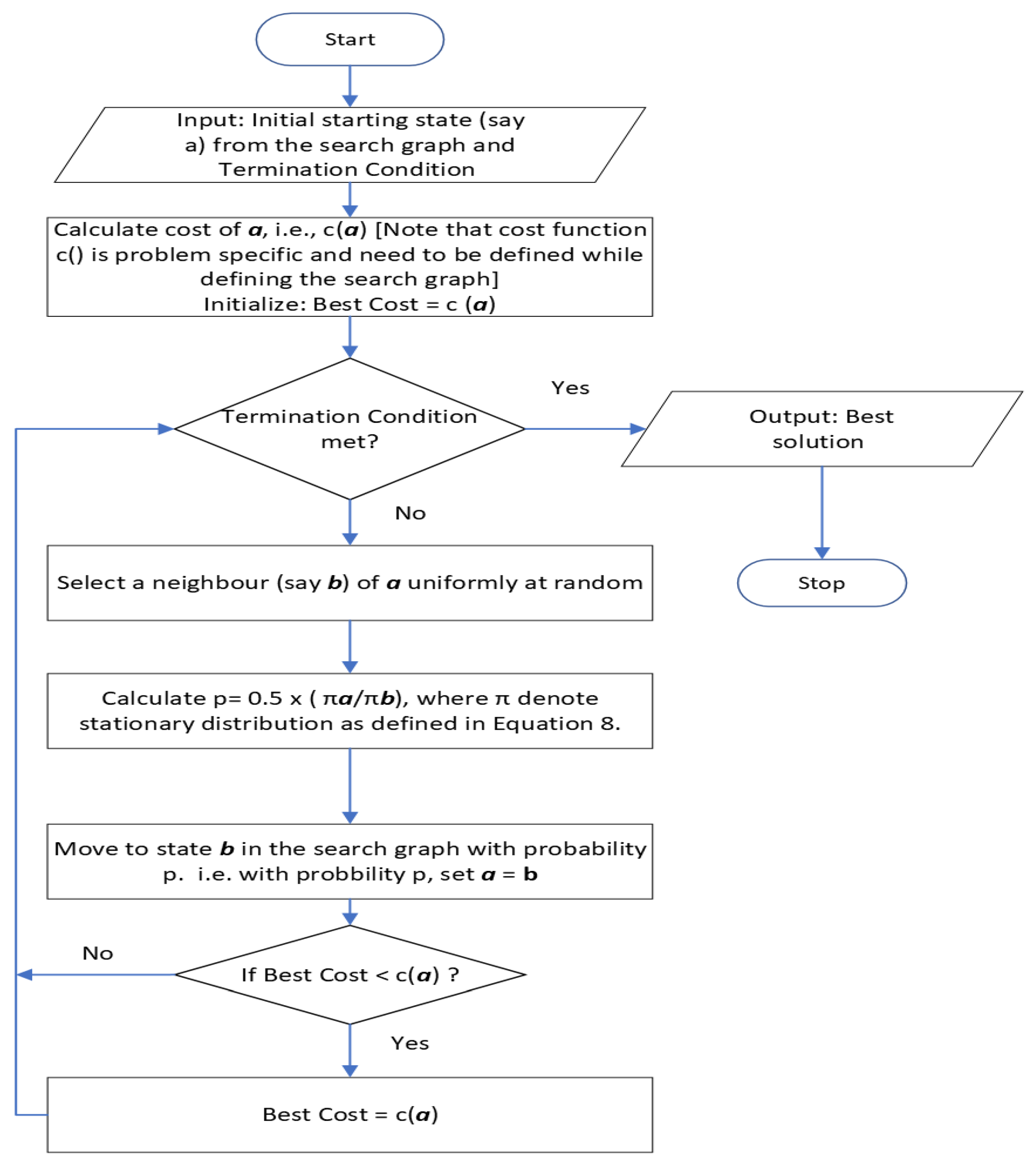
Algorithm 1 MA for Maximization Problem.

1: Input: Initial solution, i.e., any state a from the search graph $\Omega$ and terminate condition   2: Output: Final solution, i.e., a state from the search graph which has desired cost of fitness (i.e., optimum or near to optimum solution)   3: Initialize $BestCost=C\left(a\right)$, where $C\left(a\right)$ denotes the cost (or fitness) of a (Note that cost function $c(.)$ and neighborhood structure should be defined in the search graph definition for the problem at hand   4: while (Until meeting the terminate condition) do   5:     Select a neighbor b of a uniformly at random   6:     Set $a=b$ with probability $\alpha$, where $$\alpha =\frac{1}{2}.min\left(\frac{exp\left(\frac{-C\left(a\right)}{T}\right)}{exp\left(\frac{-C\left(b\right)}{T}\right)},1\right)$$   7:     if $(BestCost<C(a\left)\right)$ then   8:          $BestCost\leftarrow C\left(a\right)$   9:     end if 10:     $steps\leftarrow steps+1$ 11: end while

The MA induces MC on the state space $\Omega$ and the transition matrix $\mathbf{P}$ of MC is given as:

$$\mathbf{P}[X_{k+1}=b|X_k=a]=\left\{\begin{array}{c}0\hfill \\ (\mathrm{if} a\ne b \mathrm{and} b\notin N(a\left)\right)\hfill \\ \frac{1}{2N}·e^{-\frac{c\left(a\right)-c\left(b\right)}{T}}\hfill \\ (\mathrm{if} c(b)\le c(a) \mathrm{and} b\in N(a\left)\right)\hfill \\ \frac{1}{2N}\hfill \\ (\mathrm{if} c(b)>c(a) \mathrm{and} b\in N(a\left)\right)\hfill \\ 1-\sum _{z\ne a}\mathbf{P}[X_{k+1}=z|X_k=a]\hfill \\ (\mathrm{if} a=b)\hfill \end{array}\right.$$

(7)

where $N\left(x\right)$ denotes neighbors of a and $N={max}_{a\in \Omega }\left\{\right|N\left(a\right)\left|\right\}$, i.e., the maximum number of neighbors for any element $a\in \Omega$. The stationary distribution of the MC with the transition matrix given as Equation (7) is

$${\pi }_a=\frac{e^{-\frac{c\left(a\right)}{T}}}{{\sum }_{a\in \Omega }{e}^{-\frac{c\left(a\right)}{T}}}$$

(8)

The $1/2$ multiplication factor in transition matrix P (Equation (7)) is to ensure that with probability $1/2$ the chain remains in state x, which makes the MC lazy and aperiodic. We have assumed that the underlying search graph used by the MA is connected and hence the induced MC is irreducible. Therefore, the MC is ergodic (irreducible and aperiodic). Also, it is well known that the MC induced by the MA is reversible [52]. i.e.,

Lemma 2

(Lemma 11.8 [52]). The MC with transition matrix P (as given in Equation (7)) is irreducible and aperiodic, then it is having stationary distribution

$${\pi }_a=\frac{e^{-\frac{c\left(a\right)}{T}}}{{\sum }_{a\in \Omega }{e}^{-\frac{c\left(a\right)}{T}}}.$$

Also, the chain is reversible.

Now to use the conductance result obtained in the previous section to prove the following result.

Corollary 1.

The Conductance $\Phi \left(P\right)$ of the MC induced by the MA with transition matrix P is related to magnification $\mu (\Omega )$ as:

$$\varphi \left(P\right)\ge \frac{1}{2N}·e^{-\frac{2(C_{max}-C_{min})}{T}}·\mu (\Omega )$$

where $C_{max}$ and $C_{min}$ denotes maximum, minimum cost (fitness) respectively. Particularly for temperature parameter $T\ge k(C_{max}-C_{min})$,

$$\varphi \left(P\right)\ge \frac{1}{2N}·e^{-\frac{2}{k}}·\mu (\Omega )$$

where k is a non-zero positive constant.

Proof. 

Using Theorem 1,

$$\varphi \left(P\right)\ge P_{{u,v\in N\left(u\right)}_{min}}\frac{{\pi }_{min}}{{\pi }_{max}}·\mu (\Omega ).$$

Using Equation (7),

$$P_{{u,v\in N\left(u\right)}_{min}}\ge \frac{1}{2N}·e^{-\frac{(C_{max}-C_{min})}{T}}$$

(9)

Using Equation (8),

$$\frac{{\pi }_{min}}{{\pi }_{max}}\ge e^{-\frac{(C_{max}-C_{min})}{T}}.$$

(10)

Therefore,

$$\varphi \left(P\right)\ge \frac{1}{2N}·e^{-\frac{2(C_{max}-C_{min})}{T}}·\mu (\Omega )$$

By choosing $T\ge k(C_{max}-C_{min})$, where k is a non-zero positive constant,

$$\varphi \left(P\right)\ge \frac{1}{2N}·e^{-\frac{2}{k}}·\mu (\Omega )$$

□

Now we can establish the relationship between the mixing time of the MC induced by the MA and magnification of the search graph.

Corollary 2.

The relationship between magnification $\mu (\Omega )$ and mixing time ($t_{\mathrm{mix}}\left(\epsilon \right)$) of the reversible ergodic MC induced by the MA is given as:

$$t_{\mathrm{mix}}\left(\epsilon \right)\le \frac{16N^{2}ln{\pi }_{min}^{-1}·e^{\frac{4(C_{max}-C_{min})}{T}}}{\mu {(\Omega )}^2}$$

For $T\ge k(C_{max}-C_{min})$

$$t_{\mathrm{mix}}\left(\epsilon \right)\le \frac{16N^2·e^{\frac{4}{k}}}{\mu {(\Omega )}^2}·ln|\Omega |$$

where k is a non-zero positive constant.

Proof. 

By Theorem 2:

$$t_{\mathrm{mix}}\left(\epsilon \right)\le \frac{4ln{\pi }_{min}^{-1}}{P_{{\{u,v\in N\left(u\right)\}}_{min}}^2·\mu {(\Omega )}^2}·\frac{{\pi }_{max}^2}{{\pi }_{min}^2}$$

Using Equations (9) and (10):

$$t_{\mathrm{mix}}\left(\epsilon \right)\le \frac{16N^{2}ln{\pi }_{min}^{-1}·e^{\frac{4(C_{max}-C_{min})}{T}}}{\mu {(\Omega )}^2}$$

For $T\ge k(C_{max}-C_{min})$

$$t_{\mathrm{mix}}\left(\epsilon \right)\le \frac{16N^{2}ln{\pi }_{min}^{-1}·e^{\frac{4}{k}}}{\mu {(\Omega )}^2}$$

(11)

where k is a non-zero positive constant.

Since ${\pi }_a=\frac{e^{-\frac{c\left(a\right)}{T}}}{{\sum }_{a\in \Omega }{e}^{-\frac{c\left(a\right)}{T}}}$:

$${\pi }_{min}\ge \frac{1}{e^{\frac{(c_{max}-c_{min})}{T}}·|\Omega |}\ge \frac{1}{e^{\frac{1}{k}}|\Omega |}(\mathrm{Sin}\mathrm{ce}T\ge k(c_{max}-c_{min}))$$

(12)

Using Equations (11) and (12):

$$t_{\mathrm{mix}}\left(\epsilon \right)\le \frac{16N^2·e^{\frac{4}{k}}}{\mu {(\Omega )}^2}·ln|\Omega |$$

(13)

□

Note that the above results are proved by selecting the temperature parameter $T=k(C_{max}-C_{min})$, where k is a non zero positive constant. For $k>1$ the mixing time is $O\left(\frac{N^2·ln|\Omega |}{\mu {(\Omega )}^2}\right))$. As k tends to zero, the mixing time will become larger and larger. Hence, one has to vary the value of parameter k, where $(0<k\le 1)$ and check experimentally, for which value of k the MA gives better result. This way of selecting the temperature parameter ensures that the Markov chain associated with the Metropolis algorithm mixes rapidly. The results show that the mixing time of the MC induced by MA on the search graph is indirectly proportional to magnification of the search graph. A large magnification implies the MC induced by MA mixes rapidly. Hence it is important to design a good search space that is connected and has large magnification. This ensures that any randomized local search heuristics, if it induces reversible ergodic MCs on such a state space, it will mix rapidly, i.e., in polynomial time. A detailed block diagram representing how to apply the proposed method to a new combinatorial optimization problem is given in Figure 4.

The following section discusses the importance of the proposed results using suitable examples.

5. Importance of the Theoretical Results Obtained: Illustration Using $\mathbf{0}\mathbf{/}\mathbf{1}$-Knapsack Problem

This section discusses how the obtained results can be applied to combinatorial optimization problem. The application of the proposed work is illustrated using $0/1$-Knapsack problem, which is a well-studied hard combinatorial optimization problem in the literature [3,53,54,55]. $0/1$-Knapsack problem has vast applications. Some of the real-world applications of Knapsack problem are financial decision problems, Knapsack cryptosystems, combinatorial auctions and load-shedding in microgrid operation, etc. [56,57].

Definition 7.

$0/1$-Knapsack Problem: Let $w_1,\dots ,w_n$ and $p_1,\dots ,p_n$ denote weights and profits associated with n items, respectively. The problem is to fill a bag (or knapsack) with items in such a way that the profit earned is maximum and the weight of all the items included in the knapsack is less than the capacity of the knapsack. More formally,

$$\mathit{Maximize}Z=\sum _{i=1}^n{x}_i{p}_i$$

subject to the constraints:

$$\sum _{i=1}^n{x}_i{w}_i\le C,whereCdenotethecapacityoftheknapsackand{x}_i\in \{0,1\}:$$

$$x_i=\left\{\begin{array}{cc}1\hfill & if{i}^{th}itemisincludedintheknapsack\hfill \\ 0\hfill & Otherwise\hfill \end{array}\right.$$

Note that partial filling of items in the knapsack is not allowed, which implies either that an item can be filled in the knapsack or not. Therefore, this problem is called the $0/1$-Knapsack problem. Now by applying steps mentioned in Figure 2 and Figure 4, we show that the Markov chain associated with the random walk and the Metropolis algorithm mixes rapidly, i.e., in polynomial time for the $0/1$-Knapsack problem. The search space used by local search-based metaheuristics for this problem is given in Definition 8.

Definition 8.

(Search Space (or search graph) for $0/1$-Knapsack Problem).

• Search Space Elements (or nodes): Set of all n bit strings, where each bit in the string can take the values 1 or 0. Each node in the search graph represents n bit string;
• Neighborhood Structure: Two nodes in the search graph are adjacent to each other if the hamming distance between two string is equal to 1;
• cost (or fitness): Cost of a node is number of 1’s in the bit string. More formally, if $x=(x_1,\dots ,x_n)$ is a node in the search graph then cost $c\left(x\right)$ of x is given as $c\left(x\right)={\sum }_{i=1}^n{x}_i{p}_i$.

Let $\Omega$ denote the search space defined in the Definition 8. Then the number of search space elements (or nodes) in the search graph is equal to the total number of possible n bit binary string, which is equal to $2^n$. Therefore $|\Omega |=2^n$. As a first step, we will find the magnification of the search graph.

Proposition 1.

The magnification of the search graph for $0/1$-Knapsack problem is at least 1.

Proof. 

We prove this by using the concept of canonical path [11,41]. We describe it quickly here for better readability. For each pair of nodes, say x and y in search space $\Omega$, define a unique path ${\beta }_{x,y}$ from x to y. This unique path ${\beta }_{x,y}$ is canonical path from x to y. Let $(p,q)$ be an edge in the search graph $\Omega$, which implies p and q are neighbors in the search space (i.e, the hamming distance between them is equal to 1 (refer to Definition 8)). Now the aim is to bind the number of canonical paths passing through the edge $(p,q)$. Let $x=(x_1,\dots ,x_n)$ and $y=(y_1,\dots ,y_n)$ be any two nodes in the search graph (as per the search space in Definition 8, each node represents n bit binary string). Let $i_1,\dots ,i_k$ are indices (in increasing order), where bit values of x and y differs. Then canonical path ${\beta }_{x,y}$ is defined as $u_0=x{u}_1{u}_2\dots u_k=y$, where $u_j$ and $u_{j-1}$ are neighbors to each other ($\forall 1\le j\le k$) and they differ at $i_j$-th bit.

Let the canonical path ${\beta }_{x,y}$ pass through the edge $(p,q)=(u_{j-1},u_j)$, where $p=(y_1,y_2,\dots ,y_{j-1},x_j,\dots ,x_n)$ and $q=(y_1,y_2,\dots ,y_j,x_{j+1},\dots ,x_n)$. That means values of first j-bits of y match with p and values of last $n-j+1$-bits x match with m. Therefore, the number of canonical paths ${\beta }_{x,y}$ which passes through edge $(p,q)$ is less than or equal to

$$2^{n-i}·2^{i-1}=2^{n-1}=\frac{|\Omega |}{2}.$$

(14)

Next, we will bind magnification of the search graph: Let $S\subset \Omega$, $S\ne \pi$ and $\left|S\right|\le \frac{|\Omega |}{2}$. Let $\eta (S,\overline{S})$ denotes the set of all canonical paths ${\beta }_{x,y}$ which start at node $x\in S$ and end at node $y\in \overline{S}$, where $\overline{S}$ denote the compliment of set S. Then

$$|\eta (S,\overline{S})|=|S|\times |\overline{S}|\ge \frac{\left|S\right|·|\Omega |}{2}(\mathrm{Since}|S|<\frac{|\Omega |}{2},|\overline{S}|\ge \frac{|\Omega |}{2})$$

(15)

Note that every canonical path ${\beta }_{x}y\in \eta (S,\overline{S})$ should pass through one edge $(p,q)\in \mathcal{E}(S,\overline{S})$, where $\mathcal{E}(S,\overline{S})$ denotes the edges in the cut set $(S,\overline{S})$. From Equation (14) we know that the number of canonical paths which passes through an edge is bounded above by $\frac{|\Omega |}{2}$. Therefore,

$$|\eta (S,\overline{S})|\le |\mathcal{E}(S,\overline{S})|·\frac{|\Omega |}{2}$$

(16)

From Equations (15) and (16) we get:

$$\frac{\left|S\right|·|\Omega |}{2}\le |\eta (S,\overline{S})|\le |\mathcal{E}(S,\overline{S})|·\frac{|\Omega |}{2}$$

Therefore,

$$\mu \left(S\right)=\frac{\left|\mathcal{E}\right(S,\overline{S}\left)\right|}{\left|S\right|}\ge 1$$

Hence the proof. □

Next we show the application of our results (Theorems 1 and 2, Corollarys 1 and 2) by taking two randomized local search-based metaheuristics Random walk and MA for $0/1$-Knapsack Problem.

5.1. Mixing Time of MC Associated with Random Walk for $0/1$-Knapsack Problem

Consider a random walk on the search graph defined in Definition 8. This random walk will induce a MC on the search space. We can make this MC aperiodic by assigning self loop probability of $1/2$. From the search graph definition (Definition 8) it is clear that number of neighbors for each node is n. Since random walk selects any of the neighbor uniformly at random and move to that node, the transition probability of such a random walk can be given as follows:

$$\mathbf{P}(a,b)=\left\{\begin{array}{c}0\hfill \\ (\mathrm{if} a\ne b \mathrm{and} b\notin N(a\left)\right)\hfill \\ \frac{1}{2n}\hfill \\ (\mathrm{if} b\in N(a\left)\right)\hfill \\ 1/2\hfill \\ D(\mathrm{if} a=b)\hfill \end{array}\right.$$

(17)

Note that since it is a random walk, stationary distribution is uniform (i.e., ${\pi }_a={\pi }_b$) and ${\pi }_{a}P(a,b)={\pi }_{b}P(b,a)$. Therefore, MC is ergodic and reversible. Hence we can apply the proposed results for this chain.

Corollary 3.

Conductance and mixing time of the of MC P induced by random walk are bounded as

• Conductance $\Phi \left(P\right)\ge \frac{1}{2n}$
• Mixing Time $t_{\mathrm{mix}}\left(\epsilon \right)\le 16n^3$.

Proof. 

Using Theorem 1 and Proposition 1, we get conductance $\Phi \left(P\right)\ge \frac{1}{2n}$ (since ${\pi }_{min}={\pi }_{max}$, $N=n$, transition probability $P(a,b)=1/2n$ and $\mu \left(G\right)\ge 1$).

Using Theorem 2 we get, $t_{\mathrm{mix}}\left(\epsilon \right)\le 16n^2·ln{\pi }_{min}^{-1}$. Since $\pi =1/2^n$, we get: $t_{\mathrm{mix}}\left(\epsilon \right)\le 16n^3$. □

5.2. Mixing Time of MC Associated with the MA for $0/1$-Knapsack Problem

As discussed in Section 4, MC induced by the MA is reversible and ergodic. Transition probability for the $0/1$-Knapsack problem is given as

$$\mathbf{P}(a,b)=\left\{\begin{array}{c}0\hfill \\ (\mathrm{if} a\ne b \mathrm{and} b\notin N(a\left)\right)\hfill \\ \frac{1}{2n}·e^{-\frac{c\left(a\right)-c\left(b\right)}{T}}\hfill \\ (\mathrm{if} c(b)\le c(a) \mathrm{and} b\in N(a\left)\right)\hfill \\ \frac{1}{2n}\hfill \\ (\mathrm{if} c(b)>c(a) \mathrm{and} b\in N(a\left)\right)\hfill \\ 1-\sum _{z\ne a}\mathbf{P}[X_{k+1}=z|X_k=a]\hfill \\ (\mathrm{if} a=b)\hfill \end{array}\right.$$

(18)

We can apply the theoretical results obtained (Corollarys 1 and 2) to bound conductance and mixing time of the MC induced MA for $0/1$-Knapsack problem.

Corollary 4.

Conductance and mixing time of the of MCs P induced by the MA are bounded as

• $\Phi \left(P\right)\ge \frac{1}{2n}·e^{\frac{-2}{k}}$
• $t_{\mathrm{mix}}\left(\epsilon \right)\le 16n^3·e^{\frac{4}{k}}$ for temperature parameter $T\ge k(c_{max}-c_{min})$

Proof. 

Using Corollary 1 we get: $\Phi \left(P\right)\ge \frac{1}{2n}·e^{\frac{-2}{k}}$ for non zero positive constant k (since magnification $\mu \left(G\right)\ge 1$ and $N=n$).

Using Corollary 2 and $|\Omega |=2^n$ we get:

$$t_{\mathrm{mix}}\left(\epsilon \right)\le 16n^3·e^{\frac{4}{k}},$$

(19)

for non zero positive constant k. □

6. Conclusions

This work builds the relationship between the magnification of a search graph and the mixing time of the reversible MC induced by local search-based metaheuristics. If the search graph has large magnification, then the ergodic reversible Markov chain induced by the local search-based metaheuristics mixes rapidly in polynomial time. Using this result, it is further proved that, if the search graph has large magnification, then the MCs induced by MA mixes rapidly for a particular choice of temperature parameter. Mixing time of MC induced MA is upper bounded by $\frac{16N^2·ln|\Omega |·e^{\frac{4}{k}}}{\mu {(\Omega )}^2}$. The importance of the proposed result is illustrated by applying it to the $0/1$-Knapsack problem. The search graph for the $0/1$-Knapsack problem has a large magnification and hence the Markov chain induced by local search-based metaheuristics like random walk and Metropolis Algorithm mixes rapidly, i.e., in polynomial time. Hence, we conclude that the design of search space plays an important role in the mixing time of MC induced local search-based metaheuristics. If one can design a search graph with large magnification for a hard optimization problem, then it is worth analyzing the performance of the local search-based metaheuristics on that search graph both theoretically and experimentally. Some limitations of the proposed work are:

• The proposed theoretical results hold only if the local search-based metaheuristics can induce reversible ergodic Markov chains on the search graph.;
• Even though the Markov chain induced by the metaheuristic algorithms mixes rapidly, i.e., in polynomial time (say $T_{mix}$), one may have to take many samples to get the desired solution for the problem at hand. One sample is obtained by running local search-based metaheuristic algorithms for $T_{mix}$ amount of time. So, it would be interesting to study how many samples are needed to get the optimum or near optimum solution for the problem at hand;
• Note that the results for the Metropolis Algorithm are proved by selecting temperature parameter $T=k(C_{max}-C_{min})$, where k is a non-zero positive constant. For $k>1$ the mixing time is $O\left(\frac{N^2·ln|\Omega |}{\mu {(\Omega )}^2}\right))$. As k tends to zero, the mixing time will become larger and larger. Hence, one must vary the value of parameter k, where $(0<k\le 1)$ and check experimentally, for which the value of k the MA gives a better result.

It is also worthwhile to analyze the performance of non-local search-based metaheuristics such as Genetic algorithms, nature-inspired algorithms, and bio-inspired algorithms, etc., for combinatorial optimization problems using the search spaces with and without large magnification.

References

1. Rubin, S.H.; Bouabana-Tebibel, T.; Hoadjli, Y.; Ghalem, Z. Reusing the NP-Hard Traveling-Salesman Problem to Demonstrate That P NP (Invited Paper). In Proceedings of the 2016 IEEE 17th International Conference on Information Reuse and Integration (IRI), Pittsburgh, PA, USA, 28–30 July 2016; pp. 574–581. [Google Scholar] [CrossRef]
2. Pandiri, V.; Singh, A.; Rossi, A. Two hybrid metaheuristic approaches for the covering salesman problems. Neural Comput. Appl. 2020, 32, 15643–15663. [Google Scholar] [CrossRef]
3. Buhrman, H.; Loff Barreto, B.S.; Torenvliet, L. Hardness of Approximation for Knapsack Problems. Theory Comput. Syst. 2015, 56, 372–393. [Google Scholar] [CrossRef] [Green Version]
4. Capobianco, G.; D’Ambrosio, C.; Pavone, L.; Raiconi, A.; Vitale, G.; Sebastiano, F. A hybrid metaheuristic for the Knapsack Problem with Forfeits. Soft Comput. 2021. [Google Scholar] [CrossRef]
5. Gaspar, D.; Lu, Y.; Song, M.S.; Vasko, F.J. Simple population-based metaheuristics for the multiple demand multiple-choice multidimensional knapsack problems. Int. J. Metaheuristics 2020, 7, 330–351. [Google Scholar] [CrossRef]
6. Garey, M.R.; Johnson, D.S. Computers and Intractability; A Guide to the Theory of NP-Completeness; W. H. Freeman & Co.: New York, NY, USA, 1990. [Google Scholar]
7. Ullman, J. NP-complete scheduling problems. J. Comput. Syst. Sci. 1975, 10, 384–393. [Google Scholar] [CrossRef] [Green Version]
8. Theophilus, O.; Dulebenets, M.A.; Pasha, J.; Lau, Y.Y.; Fathollahi-Fard, A.M.; Mazaheri, A. Truck scheduling optimization at a cold-chain cross-docking terminal with product perishability considerations. Comput. Ind. Eng. 2021, 156, 107240. [Google Scholar] [CrossRef]
9. Dulebenets, M.A. A Delayed Start Parallel Evolutionary Algorithm for just-in-time truck scheduling at a cross-docking facility. Int. J. Prod. Econ. 2019, 212, 236–258. [Google Scholar] [CrossRef]
10. Gholizadeh, H.; Fazlollahtabar, H.; Fathollahi-Fard, A.M.; Dulebenets, M.A. Preventive maintenance for the flexible flowshop scheduling under uncertainty: A waste-to-energy system. Environ. Sci. Pollut. Res. 2021. [Google Scholar] [CrossRef]
11. Ajitha Shenoy, K.B.; Biswas, S.; Kurur, P.P. Metropolis algorithm for solving shortest lattice vector problem (SVP). In Proceedings of the 2011 11th International Conference on Hybrid Intelligent Systems (HIS), Melaka, Malaysia, 5–8 December 2011; pp. 442–447. [Google Scholar]
12. Goldberg, D.E. Genetic Algorithms in Search, Optimization, and Machine Learning; Addison-Wesley: New York, NY, USA, 1989. [Google Scholar]
13. Metropolis, N.; Rosenbluth, A.W.; Rosenbluth, M.N.; Teller, A.H.; Teller, E. Equation of State Calculations by Fast Computing Machines. J. Chem. Phys. 1953, 21, 1087–1092. [Google Scholar] [CrossRef] [Green Version]
14. Kirkpatrick, S.; Gelatt, C.D.; Vecchi, M.P. Optimization by Simulated Annealing. Science 1983, 220, 671–680. [Google Scholar] [CrossRef]
15. Kennedy, J.; Eberhart, R.C. Particle swarm optimization. In Proceedings of the IEEE International Conference on Neural Networks, Perth, Australia, 27 November–1 December 1995; pp. 1942–1948. [Google Scholar]
16. Dorigo, M.; Stützle, T. Ant Colony Optimization; Bradford Company: Scituate, MA, USA, 2004. [Google Scholar]
17. Mühlenthaler, M.; Raß, A.; Schmitt, M.; Wanka, R. Exact Markov chain-based runtime analysis of a discrete particle swarm optimization algorithm on sorting and OneMax. Nat. Comput. 2021. [Google Scholar] [CrossRef]
18. Yang, X.S. Metaheuristic Optimization: Algorithm Analysis and Open Problems. In Experimental Algorithms; Pardalos, P.M., Rebennack, S., Eds.; Springer: Berlin/Heidelberg, Germany, 2011; pp. 21–32. [Google Scholar]
19. Sudholt, D. Using Markov-Chain Mixing Time Estimates for the Analysis of Ant Colony Optimization. In Proceedings of the FOGA’11, 11th Workshop Proceedings on Foundations of Genetic Algorithms, Schwarzenberg, Austria, 5–8 January 2011; Association for Computing Machinery: New York, NY, USA, 2011; pp. 139–150. [Google Scholar] [CrossRef]
20. Munien, C.; Ezugwu, A.E. Metaheuristic algorithms for one-dimensional bin-packing problems: A survey of recent advances and applications. J. Intell. Syst. 2021, 30, 636–663. [Google Scholar] [CrossRef]
21. Lissovoi, A.; Witt, C. A Runtime Analysis of Parallel Evolutionary Algorithms in Dynamic Optimization. Algorithmica 2017, 78, 641–659. [Google Scholar] [CrossRef] [PubMed] [Green Version]
22. Jerrum, M.; Sinclair, A. The Markov Chain Monte Carlo Method: An Approach to Approximate Counting and Integration. In Approximation Algorithms for NP-Hard Problems; PWS Publishing Co.: Boston, MA, USA, 1996; pp. 482–520. [Google Scholar]
23. Sinclair, A.; Jerrum, M. Approximate counting, uniform generation and rapidly mixing Markov chains. Inf. Comput. 1989, 82, 93–133. [Google Scholar] [CrossRef] [Green Version]
24. Aldous, D. On the Markov Chain Simulation Method for Uniform Combinatorial Distributions and Simulated Annealing. Probab. Eng. Inf. Sci. 1987, 1, 33–46. [Google Scholar] [CrossRef]
25. Davis, T.E.; Principe, J.C. A Markov Chain Framework for the Simple Genetic Algorithm. Evol. Comput. 1993, 1, 269–288. [Google Scholar] [CrossRef]
26. Doerr, C.; Sudholt, D. Preface to the Special Issue on Theory of Genetic and Evolutionary Computation. Algorithmica 2019, 81, 589–592. [Google Scholar] [CrossRef] [Green Version]
27. Aldous, D.; Fill, J.A. Reversible Markov Chains and Random Walks on Graphs, 2002. Unfinished Monograph, Recompiled 2014. Available online: https://www.stat.berkeley.edu/~aldous/RWG/book.pdf (accessed on 1 November 2021).
28. Kwon, J. Particle swarm optimization–Markov Chain Monte Carlo for accurate visual tracking with adaptive template update. Appl. Soft Comput. 2020, 97, 105443. [Google Scholar] [CrossRef]
29. Chou, C.W.; Lin, J.H.; Yang, C.H.; Tsai, H.L.; Ou, Y.H. Constructing a Markov Chain on Particle Swarm Optimizer. In Proceedings of the 2012 Third International Conference on Innovations in Bio-Inspired Computing and Applications, Kaohsiung, Taiwan, 26–28 September 2012; pp. 13–18. [Google Scholar] [CrossRef]
30. Di Cesare, N.; Chamoret, D.; Domaszewski, M. A New Hybrid PSO Algorithm Based on a Stochastic Markov Chain Model. Adv. Eng. Softw. 2015, 90, 127–137. [Google Scholar] [CrossRef]
31. Jeong, B.; Han, J.H.; Lee, J.Y. Metaheuristics for a Flow Shop Scheduling Problem with Urgent Jobs and Limited Waiting Times. Algorithms 2021, 14, 323. [Google Scholar] [CrossRef]
32. Panteleev, A.V.; Lobanov, A.V. Application of Mini-Batch Metaheuristic Algorithms in Problems of Optimization of Deterministic Systems with Incomplete Information about the State Vector. Algorithms 2021, 14, 332. [Google Scholar] [CrossRef]
33. Zhang, Y.; Wang, J.; Li, X.; Huang, S.; Wang, X. Feature Selection for High-Dimensional Datasets through a Novel Artificial Bee Colony Framework. Algorithms 2021, 14, 324. [Google Scholar] [CrossRef]
34. Ebrahimi Moghadam, M.; Falaghi, H.; Farhadi, M. A Novel Method of Optimal Capacitor Placement in the Presence of Harmonics for Power Distribution Network Using NSGA-II Multi-Objective Genetic Optimization Algorithm. Math. Comput. Appl. 2020, 25, 17. [Google Scholar] [CrossRef] [Green Version]
35. Hedar, A.R.; Deabes, W.; Almaraashi, M.; Amin, H.H. Evolutionary Algorithms Enhanced with Quadratic Coding and Sensing Search for Global Optimization. Math. Comput. Appl. 2020, 25, 7. [Google Scholar] [CrossRef] [Green Version]
36. Juárez-Smith, P.; Trujillo, L.; García-Valdez, M.; Fernández de Vega, F.; Chávez, F. Pool-Based Genetic Programming Using Evospace, Local Search and Bloat Control. Math. Comput. Appl. 2019, 24, 78. [Google Scholar] [CrossRef] [Green Version]
37. Berberler, M.E.; Guler, A.; Nurıyev, U.G. A Genetic Algorithm to Solve the Multidimensional Knapsack Problem. Math. Comput. Appl. 2013, 18, 486–494. [Google Scholar] [CrossRef]
38. Uğur, A.; Korukoğlu, S.; Çalıskan, A.; Cinsdikici, M.; Alp, A. Genetic Algorithm Based Solution for TSP on a Sphere. Math. Comput. Appl. 2009, 14, 219–228. [Google Scholar] [CrossRef]
39. Malkiel, B.G. A Random Walk Down Wall Street; Norton: New York, NY, USA, 1973. [Google Scholar]
40. Lourenço, H.R.; Martin, O.C.; Stützle, T. Iterated Local Search; Springer: Boston, MA, USA, 2003. [Google Scholar]
41. Sinclair, A. Algorithms for Random Generation and Counting A Markov Chain Approach; Birkhauser Boston: Cambridge, MA, USA, 1993. [Google Scholar]
42. Cipra, B.A. The Best of the 20th Century: Editors Name Top 10 Algorithms. SIAM News 2000, 33. Available online: https://archive.siam.org/pdf/news/637.pdf (accessed on 15 October 2021).
43. Sanyal, S.; S, R.; Biswas, S. Necessary and Sufficient Conditions for Success of the Metropolis Algorithm for Optimization. In Proceedings of the GECCO’10, 12th Annual Conference on Genetic and Evolutionary Computation, Portland, OR, USA, 7–11 July 2010; Association for Computing Machinery: New York, NY, USA, 2010; pp. 1417–1424. [Google Scholar] [CrossRef]
44. Rashkovskiy, S. Monte Carlo solution of combinatorial optimization problems. Dokl. Math. 2016, 94, 720–724. [Google Scholar] [CrossRef]
45. Bazavov, A.; Berg, B.A.; Zhou, H. Application of Biased Metropolis Algorithms: From protons to proteins. Math. Comput. Simul. 2010, 80, 1056–1067. [Google Scholar] [CrossRef] [Green Version]
46. Marze, N.A.; Roy Burman, S.S.; Sheffler, W.; Gray, J.J. Efficient flexible backbone protein–protein docking for challenging targets. Bioinformatics 2018, 34, 3461–3469. [Google Scholar] [CrossRef] [PubMed] [Green Version]
47. Yang, J.; Roberts, G.O.; Rosenthal, J.S. Optimal scaling of random-walk metropolis algorithms on general target distributions. Stoch. Process. Their Appl. 2020, 130, 6094–6132. [Google Scholar] [CrossRef]
48. Ajitha Shenoy, K.B.; Biswas, S.; Kurur, P.P. Efficacy of the Metropolis Algorithm for the Minimum-Weight Codeword Problem Using Codeword and Generator Search Spaces. IEEE Trans. Evol. Comput. 2020, 24, 664–678. [Google Scholar] [CrossRef]
49. Ajitha Shenoy, K.B.; Biswas, S.; Kurur, P.P. Performance of Metropolis Algorithm for the Minimum Weight Code Word Problem. In Proceedings of the GECCO ’14, 2014 Annual Conference on Genetic and Evolutionary Computation, Vancouver, BC, Canada, 12–16 July 2014; Association for Computing Machinery: New York, NY, USA, 2014; pp. 485–492. [Google Scholar] [CrossRef]
50. Tiana, G.; Sutto, L.; Broglia, R. Use of the Metropolis algorithm to simulate the dynamics of protein chains. Phys. A Stat. Mech. Appl. 2007, 380, 241–249. [Google Scholar] [CrossRef] [Green Version]
51. Norris, J.R. Markov Chains; Cambridge Series in Statistical and Probabilistic Mathematics; Cambridge University Press: Cambridge, UK, 1998; pp. I–XVI, 1–237. [Google Scholar]
52. Mitzenmacher, M.; Upfal, E. Probability and Computing: Randomized Algorithms and Probabilistic Analysis; Cambridge University Press: New York, NY, USA, 2005. [Google Scholar]
53. Connolly, D. Knapsack Problems: Algorithms and Computer Implementations. J. Oper. Res. Soc. 1991, 42, 513. [Google Scholar] [CrossRef]
54. Pisinger, D. Where are the hard knapsack problems? Comput. Oper. Res. 2005, 32, 2271–2284. [Google Scholar] [CrossRef]
55. Assi, M.; Haraty, R.A. A Survey of the Knapsack Problem. In Proceedings of the 2018 International Arab Conference on Information Technology (ACIT), Werdanye, Lebanon, 28–30 November 2018; pp. 1–6. [Google Scholar] [CrossRef]
56. Choi, S.; Park, S.; Kim, H.M. The Application of the 0-1 Knapsack Problem to the Load-Shedding Problem in Microgrid Operation. In Control and Automation, and Energy System Engineering; Kim, T.H., Adeli, H., Stoica, A., Kang, B.H., Eds.; Springer: Berlin/Heidelberg, Germany, 2011; pp. 227–234. [Google Scholar]
57. Kellerer, H.; Pferschy, U.; Pisinger, D. Some Selected Applications. In Knapsack Problems; Springer: Berlin/Heidelberg, Germany, 2004; pp. 449–482. [Google Scholar] [CrossRef]
Figure 1. Flow chart representing local search-based metaheuristic algorithm.
Mathematics 10 00047 g001
Figure 2. Block diagram representing how to apply the proposed method for a new combinatorial Optimization Problem.
Mathematics 10 00047 g002
Figure 3. Metropolis Algorithm.
Mathematics 10 00047 g003
Figure 4. Block Diagram representing how to apply the Metropolis algorithm for a new combinatorial Optimization Problem.
Mathematics 10 00047 g004
Publisher’s Note: MDPI stays neutral with regard to jurisdictional claims in published maps and institutional affiliations.