Darcy–Brinkman–Forchheimer Model for Nano-Bioconvection Stratified MHD Flow through an Elastic Surface: A Successive Relaxation Approach

Abstract

The present study deals with the Darcy–Brinkman–Forchheimer model for bioconvection-stratified nanofluid flow through a porous elastic surface. The mathematical modeling for MHD nanofluid flow with motile gyrotactic microorganisms is formulated under the influence of an inclined magnetic field, Brownian motion, thermophoresis, viscous dissipation, Joule heating, and stratifi-cation. In addition, the momentum equation is formulated using the Darcy–Brinkman–Forchheimer model. Using similarity transforms, governing partial differential equations are reconstructed into ordinary differential equations. The spectral relaxation method (SRM) is used to solve the nonlinear coupled differential equations. The SRM is a straightforward technique to develop, because it is based on decoupling the system of equations and then integrating the coupled system using the Chebyshev pseudo-spectral method to obtain the required results. The numerical interpretation of SRM is admirable because it establishes a system of equations that sequentially solve by providing the results of the first equation into the next equation. The numerical results of temperature, velocity, concentration, and motile microorganism density profiles are presented with graphical curves and tables for all the governing parametric quantities. A numerical comparison of the SRM with the previously investigated work is also shown in tables, which demonstrate excellent agreement.

1. Introduction

In 1995, Choi and Eastman [1] developed the concept of a “nanofluid”, which refers to the suspension of nanometer-sized particles in a base fluid containing nanoparticles with diameters smaller than 100 nm. Choi and Eastman [1] proved that nanofluids enhance the thermal conductivity of the base fluids. Nanofluids have received a lot of attention in engineering sectors because of their thermal enhancing features. The strong link between bulk materials and molecular interactions is produced by nanofluid mechanics. Nanofluids have various applications, including as productive energy sources, solar cells, and vehicle engines, as well as in electronic circuits to enhance the cooling process [2]. To simulate the flow of nanofluids and ensure that the influence of thermophoresis and Brownian motility is effective, Buongiorno’s nanofluid model [3] is employed. Tiwari and Das [4] used a solid volume fraction of fragments to offer an alternative modelling approach for assessing enhancement in the thermal conductivity of nanofluids. Kakaç and Pramuanjaroenkij [5] gave an in-depth analysis on convective transport in nanofluids. A stable boundary-layer nanofluid flowing past a semi-infinite moveable sheet was studied by Bachok et al. [6]. The flow of a convective boundary-layer nanofluid past a stretched plate was examined by Makinde and Aziz [7]. Haddad et al. [8] investigated the natural convection of nanofluids under the influence of Brownian motion and thermophoresis parameters. The efficiency of MHD mixed-convection heat transmission in nanofluid flowing from a conduit with sinusoidal walls was determined by Rashidi et al. [9]. Using Buongiorno’s models, Kefayati [10] analyzed the natural convection and entropy generation of a non-Newtonian nanofluid moving through a prior cavity.

The study of magnetohydrodynamics (MHD) has a wide range of applications in engineering, including in atomic reactor cooling, the petroleum industry, boundary control in crystallite production and aerospace engineering, MHD power generators, and MHD detectors, among others. The effects of magnetic fields on nanofluid flow are also important in applied physics, medical science, and engineering. Ibrahim and Shankar [11] investigated boundary layer flow with MHD and heat transfer with the simultaneous impacts of velocity, temperature, and solutal slip boundary conditions. The magnetohydrodynamic effectiveness of nanofluid stagnation point flow across a stretching sheet was examined by Ibrahim et al. [12]. Mabood et al. [13] looked at magnetohydrodynamic boundary layer nanofluid flow with heat transfer over a nonlinearly stretched surface. Khan et al. [14] studied the Carreau nanofluid flow towards a stretched cylinder under the influence of Joule heating. Metri et al. [15] performed a Lie group analysis for MHD fluid flow with Joule heating and heat transfer. Slip effects on MHD nanofluid flow through a porous disk with oscillation have been studied by Rauf et al. [16]. A numerical investigation has been performed by Subhani and Nadeem [17] on MHD micropolar hybrid nanofluid flow through a porous medium. A stability analysis on MHD hybrid nanofluid flow with quadratic velocity from a stretching/shrinking sheet was explored by Zainal et al. [18].

Nanofluid flow through porous media has significant importance in different engineering applications, including thermal energy transport, storage systems, nuclear waste disposal systems, and geothermal systems [19]. Moreover, porous media is also applicable in energy converting devices, shale reservoirs, hydrogen storage systems, and membrane-based water desalination towards reverse osmosis. Therefore, in view of such importance, many authors have investigated nanofluid flow through porous media. For instance, Hassan et al. [20] investigated the mechanism of a wavy porous medium filled with nanofluids. They used the Darcy law and the Dupuit–Forchheimer model to formulate the mathematical modeling. Izadi et al. [21] used hybrid nanofluids to examine natural convection flow through a porous medium under magnetic effects. Eid and Nafe [22] elaborated the impact of slip, magnetic field, heat generation and Darcy law using hybrid nanofluids. Ying et al. [23] presented a thermo-hydraulic analysis with a salt-based nanofluid moving through a porous absorber tube. Loganathan et al. [24] described the importance of the Darcy–Forchheimer model for entropy generation using a third-grade nanofluid.

Bioconvection patterns, which are aggregate processes, usually occur because of the up-swimming of micro-organisms that are less dense than water in suspensions. When the upper portion of the suspension becomes excessively dense due to the accumulation of microorganisms, the suspension does not remain stable, and the microorganisms fall, causing bioconvection. Bioconvection is used in a wide range of applications [25], such as sustainable fuel technology, biological polymer synthesis, the pharmaceutical industry, biotechnology, and biosensors. Rashad and Nabwey [26] used the implicit finite difference approach to investigate mixed bioconvection nanofluid flow towards a stretchy cylinder with convective boundary conditions. The behaviour of bioconvection flow across a porous medium filled with nanofluid was studied by Ahmad et al. [27]. Alshomrani [28] used numerical computations to determine the bioconvection of a viscoelastic nanofluid under magnetic dipole suspension of microorganisms. Habib et al. [29] compared different fluid models, including Maxwell, Williamson, micropolar nanofluids, and bioconvection processes. They investigated the stretched geometrical configurations to see the effects of activation energy and double diffusion. Koriko et al. [30] used a thixotropic model traveling across a vertical surface to investigate a magnetized bioconvection nanofluid.

The minimum amount of energy required to move interposition particles through a class of chemical procedures or formations is known as activation energy. E_a is the standard abbreviation for activation energy, which is measured in kcal/mol/KJ/mol. Oil storage, geothermal engineering, food refining, chemical engineering, and mechanochemistry all employ this concept. Bestman [31] investigated the natural convective flow of binate amalgamation via a porous zone and activation energy. Makinde et al. [32] investigated time-varying natural convection phenomenality using activation energy and an n^th-order reaction. Hamid et al. [33] investigated the effect of activation energy on time-varying Magneto–Williamson nanofluid flow. Irfan et al. [34] demonstrated the implications of non-linear mixed convection and chemical reactions in a 3D radiative Carreau nanofluid flowing with activation energy. Zeeshan et al. [35] analyzed the performance of activation energy on Couette–Poiseuille flow in nanofluids with chemical reaction and convective boundary conditions. Recently, Zhang et al. [36] studied nonlinear nanofluid flow with activation energy and Lorentz force through a stretched surface using a spectral approach.

Based on the aforementioned existing literature, the major goal of this study is to determine the MHD bioconvection stratified nanofluid flow across a horizontal extended surface with activation energy. The mathematical modeling for MHD nanofluid flow with motile gyrotactic microorganisms is formulated under the influence of an inclined magnetic field, Brownian motion, thermophoresis, viscous dissipation, Joule heating, and stratification. Furthermore, the momentum equation is formulated using the Darcy–Brinkman–Forchheimer model. The governing partial differential equations are transformed into ordinary differential equations using similarity transforms. The resultant nonlinear, coupled differential equations are numerically solved using the spectral relaxation method (SRM). The SRM algorithm’s defining advantage is that it divides a large, coupled set of equations into smaller subsystems that can be handled progressively in a very computationally efficient and effective way. The proposed methodology, SRM, showed that this method is accurate, easy to develop, convergent, and highly efficient when compared with other numerical/analytical methods [37,38,39] to solve nonlinear problems. The numerical solutions for the magnitudes of velocity, concentration, temperature, and motile microbe density are calculated using the SRM algorithm. The graphical behaviors of the most important parametric parameters in the current inspection are provided and analyzed in detail.

2. Mathematical Model

Consider a bi-dimensional steady mixed convective boundary layer nanofluid flowing over a horizontally stretchable surface, as shown in Figure 1. An inclined magnetic field $B_0$ is enforced on the horizontally fluid layer, and the effect of the induced magnetic field is disregarded due to confined comparing to the extraneous magnetic field, where the influence of the electric field is not present. The surface is considered to be stretchable to ${\tilde{U}}_w=d\overline{x}$, as linear stretching velocity together with $d>0$ is a constant, and the stretchable surface is alongside the y-axis. The surface concentration $C_w$, the concentration of microorganisms $N_w$ and temperature $T_w$ on the horizontally surface are presumed to be constant and bigger than the ambient concentration $C_{\infty }$, ambient concentration of microorganisms $N_{\infty }$ and temperature $T_{\infty }$. The effects of Joule heating, viscous dissipation, and stratification on the heat, mass, and motile microbe transferal rate are investigated. The water-based nanofluid contains nanoparticles and bacteria. We also hypothesize that nanoparticles had no effect on swimming microorganisms’ velocity and orientation. As a result, the following governing equations of continuity, momentum, energy, nanoparticle concentration, and microorganisms may be established for the aforementioned situation under boundary layer approximations. In the influence of body forces, the basic equations for immiscible and irrotational flows are as follows [40]:

$$\frac{\partial \check{u}}{\partial \overline{x}}+\frac{\partial \check{v}}{\partial \overline{y}}=0,$$

(1)

$$\check{u}\frac{\partial \check{u}}{\partial \overline{x}}+\check{v}\frac{\partial \check{u}}{\partial \overline{y}}=\frac{\mu }{\rho }\frac{{\partial }^2\check{u}}{\partial {\overline{y}}^2}-\frac{\sigma B_0^2}{\rho }{\sin }^2\alpha \check{u}+\frac{1}{\rho }\left[\overline{\mathrm{g}}\beta \rho \left(T-T_{\infty }\right)\left(1-C_{\infty }\right)-\overline{\mathrm{g}}\left({\rho }_p-\rho \right)\left(C-C_{\infty }\right)-\overline{\mathrm{g}}{\beta }_N\left({\rho }_m-\rho \right)\left(N-N_{\infty }\right)\right]-\frac{\nu }{k}\check{u}-\frac{F_c}{\sqrt{k}}{\check{u}}^2,$$

(2)

$$\left(\check{u}\frac{\partial T}{\partial \overline{x}}+\check{v}\frac{\partial T}{\partial \overline{y}}\right)=\frac{k}{\rho c_p}\frac{{\partial }^{2}T}{\partial {\overline{y}}^2}+\frac{{\left(\rho c_p\right)}_p}{\rho c_p}\left[D_B\frac{\partial T}{\partial \overline{y}}\frac{\partial C}{\partial \overline{y}}+\frac{D_T}{T_{\infty }}{\left(\frac{\partial T}{\partial \overline{y}}\right)}^2\right]+\frac{\mu }{\rho c_p}{\left(\frac{\partial \check{u}}{\partial \overline{y}}\right)}^2+\frac{\sigma B_0^2}{\rho c_p}{\sin }^2\alpha {\check{u}}^2,$$

(3)

$$\check{u}\frac{\partial C}{\partial \overline{x}}+\check{v}\frac{\partial C}{\partial \overline{y}}=D_B\frac{{\partial }^{2}C}{\partial {\overline{y}}^2}+\frac{D_T}{T_{\infty }}\left(\frac{{\partial }^{2}T}{\partial {\overline{y}}^2}\right)-k_r^2\left(C-C_{\infty }\right){\left(\frac{T}{T_{\infty }}\right)}^{m_1}\exp \left(\frac{-E_a}{k_{0}T}\right),$$

(4)

$$\check{u}\frac{\partial N}{\partial \overline{x}}+\check{v}\frac{\partial N}{\partial \overline{y}}+\frac{b{W}_C}{\left(C_w-C_{\infty }\right)}\frac{\partial }{\partial \overline{y}}\left(N\frac{\partial C}{\partial \overline{y}}\right)=D_m\frac{{\partial }^{2}N}{\partial {\overline{y}}^2},$$

(5)

The following are the corresponding boundary conditions:

$$\left.\begin{array}{c}\check{u}=U_w=d\overline{x},\check{v}=0, T=T_w=T_0+b_1\overline{x},C=C_w=C_0+d_1\overline{x},\\ N=N_w=N_0+e_1\overline{x}, at \overline{y}=0,\end{array}\right\}$$

(6)

$$\left.\begin{array}{c}\check{u}\to 0, T=T_{\infty }=T_0+b_2\overline{x},C=C_{\infty }=C_0+d_2\overline{x},\\ N=N_{\infty }=N_0+e_2\overline{x}, as \overline{y}\to \infty .\end{array}\right\}$$

(7)

where $\sigma$, $k$ are the electrical and thermal conductivities of the fluid; the inclination angle of the magnetic field is $\alpha$; gravitational acceleration is $\overline{\mathrm{g}}$; the magnetic field intensity is $B_0$; the volume expansion coefficient is $\beta$; $\check{u}$ and $\check{v}$ are the velocity components for the $\overline{x}$ and $\overline{y}$ directions, successively; the densities of nanofluid, nanoparticles, and microorganism’s particles, respectively, are $\rho$, ${\rho }_p$, and ${\rho }_m$; the temperature is represented by $T$, the concentration of nanoparticles is $C$; the concentration of microorganisms is indicated by $N$; and the reference temperature, concentration of nanoparticles, and concentration of microorganisms are $T_0, C_0, \mathrm{and} N_0$, respectively. The power-law index is represented by $\overline{\mathrm{g}}$; $\mathsf{\Gamma }$ is the time constant; $\nu$ is the kinematic viscosity; $T$ is the temperature; $T_w$, $C, \mathrm{and} C_{\infty }$ are the concentration susceptibility; $D_B$ and $D_T$ describe the Brownian diffusion coefficient and the thermophoresis diffusion coefficient, respectively; $c_p$ represents the specific heat; $\alpha$ is the inclination angle; $F_c$ indicates the Forchheimer coefficient; $k_r$ is the chemical reaction ratio; $E_a$ indicates the activation energy; $k_0$ is the Boltzmann constant; and $b_1, c_1, d_1, \mathrm{and} e_1$ are the dimensionless constants.

The following similarity transformations are employed for further mathematical formulation:

$$\left.\begin{array}{c}\psi =\overline{x}\sqrt{d\nu }F\left(\eta \right), \eta =\sqrt{\frac{d}{\nu }} \overline{y}, \theta \left(\eta \right)=\frac{T-T_{\infty }}{T_w-T_0},\\ \varphi \left(\eta \right)=\frac{C-C_{\infty }}{C_w-C_0}, \Phi \left(\eta \right)=\frac{N-N_{\infty }}{N_w-N_0}, \check{u}=U_w{F}^{’}\left(\eta \right),\check{v}=-\sqrt{U_w}F\left(\eta \right),\end{array}\right\}$$

(8)

The stream functions are described as follows:

$$\check{u}=\frac{\partial \psi }{\partial \overline{y}}, \check{v}=-\frac{\partial \psi }{\partial \overline{x}}.$$

(9)

We obtain the following governing equations system by plugging Equation (8) into Equations (1)–(7):

$$F^{’’’}+F{F}^{’’}-F^{’2}-Ha{\sin }^2\alpha F^{’}+G_r\left[\theta -N_r\varphi -R_b\Phi \right]-{\beta }_D{F}^{\prime }-F_r{F}^{’2}=0,$$

(10)

$${\theta }^{″}+P_r\left\{F{\theta }^{\prime }-F^{\prime }\theta +E_c{F}^{’’2}-S{F}^{\prime }\right\}+N_b \varphi ’{\theta }^{\prime }+N_t\theta {’}^2+E_{c}Ha{\sin }^2\alpha F^{’2}=0,$$

(11)

$${\varphi }^{″}+L_e\left\{F{\varphi }^{’}-F^{\prime }\varphi -Q{F}^{\prime }-\omega {\left(1+\delta \theta \right)}^{m_1}{e}^{\left(\frac{-E}{1+\delta \theta }\right)}\varphi \right\}+\frac{N_t}{N_b}{\theta }^{″}=0,$$

(12)

$${\Phi }^{″}+L_b\left\{F{\Phi }^{\prime }-F^{\prime }\Phi -B{F}^{\prime }\right\}-P_e\left\{\left[\Phi +\Omega \right]{\varphi }^{″}+{\varphi }^{\prime }{\Phi }^{\prime }\right\}=0.$$

(13)

These are their relative boundary conditions:

$$\left.\begin{array}{c}F\left(0\right)=0,F^{\prime }\left(0\right)=1,\theta \left(0\right)=1-S, \varphi \left(0\right)=1-Q,\Phi \left(0\right)=1-B\\ F^{\prime }\left(\infty \right)=0, \theta \left(\infty \right)=\varphi \left(\infty \right)=\Phi \left(\infty \right)=0.\end{array}\right\}.$$

(14)

and

$$\begin{gathered} Ha=\frac{\sigma B_0{}^2}{\rho a}, {\beta }_D=\frac{\nu }{ak} , N_r=\frac{\left({\rho }_p-\rho \right)\left(C_w-C_0\right)}{\left(1-C_{\infty }\right)\left(T_w-T_0\right)\rho \beta }, \\ {G}_r=\frac{\overline{\mathrm{g}}\beta \left(1-C_{\infty }\right)\left(T_w-T_0\right)}{a{U}_w}, F_r=\frac{F_c{U}_w}{a\sqrt{k}},E_c=\frac{U_w^2}{c_p\left(T_w-T_0\right)} \\ R_b=\frac{{\beta }_N\left({\rho }_m-\rho \right)\left(N-N_{0 }\right)}{\left(1-C_{\infty }\right)\left(T_w-T_0\right)\rho \beta }, P_r=\frac{\mu c_p}{\kappa }, N_t=\frac{\tau D_T\left(T_w-T_0\right)}{\alpha T_{\infty }}, \\ {N}_b=\frac{\tau D_B\left(C_w-C_0\right)}{\alpha },\omega =\frac{k_r{}^2}{a}, L_e=\frac{\nu }{D_B}, \delta =\frac{\left(T_w-T_0\right)}{T_{\infty }}, E=\frac{E_a}{k_0{T}_{\infty }}, \\ {L}_b=\frac{\nu }{D_m}, \mathsf{\Omega }=\frac{N_{\infty }}{\left(N_w-N_0\right)}, P_e=\frac{b{W}_C}{D_m},S=\frac{b_2}{b_1},Q=\frac{d_2}{d_1}, B=\frac{e_2}{e_1} . \end{gathered}$$

where the Hartmann number is denoted by $Ha$, the permeability parametric quantity is denoted by ${\beta }_D$, the buoyancy proportion parameter is denoted by $N_r$, the mixed convection parametric quantity is denoted by $G_r$, the Darcy–Brinkman–Forchheimer parameter is denoted by $F_r$, the Eckert number is denoted by $E_c$, the bioconvection Rayleigh number is denoted by $R_b$, the Prandtl number is denoted by $P_r$, the thermophoresis parameter is denoted by $N_t$, the Brownian motion parameter is denoted by $N_b$, $\omega$ is the chemical reaction constant, the Lewis number is denoted by $L_e$, $\delta$ is the relatively temperature parameter, $E$ is the parameter for activation energy, the bioconvection Lewis number is $L_b$, $\mathsf{\Omega }$ is the concentration of the microorganisms’ variance parametric quantity, the bioconvection Peclet number is denoted by $P_e$, the thermal stratification parameter is denoted by $S$, the mass stratification parameter is denoted by $Q$, and the motile density stratification parameter is denoted by $B$.

The significant physical parametric quantities in the current investigation, i.e., the skin friction coefficient $C_F$, the local Sherwood number $S{h}_{\overline{x}}$, the local Nusselt number $N{u}_{\overline{x}}$, and the local density of motile microorganisms $N{n}_{\overline{x}}$, are written as:

$$\frac{R{e}_{\overline{x}}^{\frac{1}{2}}}{2}{C}_F=F^{″}\left(0\right), \frac{N{u}_{\overline{x}}}{R{e}_{\overline{x}}^{\frac{1}{2}}}=-{\theta }^{\prime }\left(0\right),\frac{S{h}_{\overline{x}}}{R{e}_{\overline{x}}^{1/2}}=-{\varphi }^{\prime }\left(0\right), \frac{N{n}_x}{R{e}_{\overline{x}}^{1/2}}=-{\Phi }^{\prime }\left(0\right).$$

(15)

where $R{e}_{\overline{x}}=\frac{\overline{x}{U}_w}{\nu }$ represents the Reynolds number.

3. Numerical Method

3.1. The SRM Scheme and Its Elementary Notion

Assuming a set of non-linear ordinary differential equations in unknown functions, i.e., $f_i\left(\zeta \right)$, $i=1, 2, \dots , n$ where $\zeta \in \left[a,b\right]$ is the dependent variable, a vector $F_i$ is established for a vector of derivatives of the variable $f_i$ for $\zeta$ as follows:

$${\mathbf{F}}_i\left(\zeta \right)=\left[ f_i{}^{\left(0\right)}, f_i{}^{\left(1\right)}\dots f_i{}^{\left(p\right)},,\dots f_i{}^{\left(m\right)}\right]$$

(16)

where $f_i{}^{\left(0\right)}=f_i$, $f_i{}^{\left(p\right)}$ is the p^th differential of $f_i$ to $\zeta$, and $f_i{}^{\left(m\right)}$ is the topmost differential. The system is rewritten as the summation of linear and non-linear segments as follows:

$$\mathcal{L}\left[{\mathit{F}}_1,{\mathit{F}}_2,\dots ,{\mathit{F}}_r \right]+Ñ\left[{\mathit{F}}_1,{\mathit{F}}_2,\dots ,{\mathit{F}}_r \right]={\mathcal{G}}_k\left(\zeta \right), k=1, 2, \dots , r$$

(17)

where ${\mathcal{G}}_k\left(\zeta \right)$ is a known function of $\zeta$. Equation (17) is solved subject to two-point boundary conditions, which can be symbolized as:

$${\displaystyle \sum }_{j=1}^m{\displaystyle \sum }_{p=0}^{m_{j-1}}{\alpha }_{\upsilon ,j}^{\left(p\right)}{f}_j^{\left(p\right)}\left(a\right)=l_{a,\upsilon }, \upsilon =1,2,\dots ,r_a$$

(18)

$${\displaystyle \sum }_{j=1}^m{\displaystyle \sum }_{p=0}^{m_{j-1}}{\beta }_{\upsilon ,j}^{\left(p\right)}{f}_j^{\left(p\right)}\left(b\right)=l_{b,\sigma }, \sigma =1,2,\dots ,r_b$$

(19)

Here, ${\alpha }_{\upsilon ,j}^{\left(p\right)}$ and ${\beta }_{\upsilon ,j}^{\left(p\right)}$ are the coefficient constants of $f_j{}^{\left(p\right)}$ in the boundary conditions, and ${\zeta }_a$, ${\zeta }_a$ are the boundary conditions at $a$ and $b$, sequentially.

Now, starting from the initial approximation ${\mathit{F}}_{1,0},{\mathit{F}}_{2,0},\dots ,{\mathit{F}}_{r,0}$, the iterative method is achieved as:

$${\mathcal{L}}_1\left[{\mathit{F}}_{1,r+1},{\mathit{F}}_{2, r+1},\dots ,{\mathit{F}}_{r,r+1} \right]+{Ñ}_1\left[{\mathit{F}}_{1,r},{\mathit{F}}_{2,r},\dots ,{\mathit{F}}_{r,r} \right]={\mathcal{G}}_1\left(\zeta \right),$$

(20)

$${\mathcal{L}}_2\left[{\mathit{F}}_{1,r+1},{\mathit{F}}_{2, r+1},\dots ,{\mathit{F}}_{r,r+1} \right]+{Ñ}_2\left[{\mathit{F}}_{1,r},{\mathit{F}}_{2,r},\dots ,{\mathit{F}}_{r,r} \right]={\mathcal{G}}_2\left(\zeta \right),$$

(21)

$$⋮⋮ ⋮ ⋮ ⋮⋮ ⋮ ⋮$$

$${\mathcal{L}}_{r-1}\left[{\mathit{F}}_{1,r+1},{\mathit{F}}_{2, r+1},\dots ,{\mathit{F}}_{r,r+1} \right]+{Ñ}_{r-1}\left[{\mathit{F}}_{1,r},{\mathit{F}}_{2,r},\dots ,{\mathit{F}}_{r,r} \right]={\mathcal{G}}_{r-1}\left(\zeta \right),$$

(22)

$${\mathcal{L}}_r\left[{\mathit{F}}_{1,r+1},{\mathit{F}}_{2, r+1},\dots ,{\mathit{F}}_{r,r+1} \right]+{Ñ}_r\left[{\mathit{F}}_{1,r},{\mathit{F}}_{2,r},\dots ,{\mathit{F}}_{r,r} \right]={\mathcal{G}}_r\left(\zeta \right),$$

(23)

where ${\mathit{F}}_{i,r+1}$ and ${\mathit{F}}_{i,r}$ are the approximations of ${\mathit{F}}_i$ for the current and precedent iterations, consecutively. We state that Equations (20)–(23) establish a set of $n$ linear decoupled equations to be resolved iteratively for $r=1, 2, . . .$. These iterations commence with an initial approximation, ${\mathit{F}}_{i,0}$, that conforms to boundary conditions. The iterations are continual until the convergence is achieved.

Now, the Chebyshev pseudospectral method [41] is implemented at this stage over Equations (20)–(23). The differentiation matrix is defined as the following:

$$\frac{d{f}_i\left({\zeta }_l\right)}{d\zeta }={\displaystyle \sum }_{K=0}^N{\mathbf{D}}_{lk}{f}_i\left({\mathsf{\tau }}_K\right)=\mathbf{D}{\mathit{F}}_i, l=0,\dots , N$$

(24)

where $N+1$ indicates the number of collocation points, $\mathbf{D}=2D/\left(b-a\right)$ and $\mathbf{F}={\left[F\left({\zeta }_0\right), F\left({\zeta }_1\right), . . . ,F\left({\zeta }_N\right) \right]}^T$ are the vector functions of the collocation points and $D$ for higher-order derivatives is accomplished in the power as given by:

$$f_j{}^{\left(p\right)}=D^p{F}_i$$

(25)

Thus, for the system of Equations (20)–(23), the previously known functions decouple the system of equations, and an efficient iteration scheme is established to generate accurate results.

3.2. Solutions by SRM Technique

The SRM technique is ready to operate on the governing system of differential equations that demand the lowering of the orders in Equation (10). We suppose $F^{\prime }=G$; then Equations (10)–(13) give:

$$G^{’’}+F{G}^{’}-G^2-Hasi{n}^2\alpha G+G_r\left(\theta -N_r\mathrm{\varphi }-R_b\mathsf{\Phi }\right)-{\beta }_{D}G-F_r{G}^2=0,$$

(26)

$${\theta }^{″}+P_r\left\{F{\theta }^{\prime }-G\theta +E_c{G}^{’2}-SG+E_{c}Hasi{n}^2\alpha G^2\right\}+N_b \mathit{\varphi }’{\theta }^{\prime }+N_t\theta {’}^2=0,$$

(27)

$${\mathit{\varphi }}^{″}+L_e\left\{F{\mathit{\varphi }}^{’}-G\mathit{\varphi }-QG-\omega {\left(1+\delta \theta \right)}^{m_1}{e}^{\left(\frac{-E}{1+\delta \theta }\right)}\mathit{\varphi }\right\}+\frac{N_t}{N_b}{\theta }^{″}=0,=0$$

(28)

$$\mathsf{\Phi } ″+L_b\left\{F \mathsf{\Phi } \prime -G\mathsf{\Phi }-BG\right\}-P_e\left\{\left[\mathsf{\Phi }+\mathsf{\Omega }\right]{\mathsf{\varphi }}^{″}+{\mathsf{\varphi }}^{\prime } \mathsf{\Phi } \prime \right\}=0.$$

(29)

Now, we apply the notion of the Gauss–Seidel relaxation scheme to decouple the reduced system in the below mode:

$$F{’}_{s+1}=G_s,$$

(30)

$${G^{″}}_{s+1}+F_s{G^{\prime }}_{s+1}-\left\{Hasi{n}^2\alpha +{\beta }_D\right\}{G}_{s+1}=G^2{}_s+F_r{G}^2{}_s-G_r\left({\theta }_s-N_r{\mathsf{\varphi }}_s-R_b{\mathsf{\Phi }}_s\right),$$

(31)

$${{\theta }^{″}}_{s+1}+P_r\left\{F_{s+1}{{\theta }^{\prime }}_{s+1}-G_{s+1}{\theta }_{s+1}-S{G}_{s+1}+E_c{G^{\prime }}^2{}_{s+1}+E_{c}Hasi{n}^2\alpha G^2{}_{s+1}\right\}+N_b {\mathsf{\varphi }}_s’{{\theta }^{\prime }}_{s+1}+N_t{{\theta }^{\prime }}^2{}_{s+1}=0,$$

(32)

$${{\mathsf{\varphi }}^{″}}_{s+1}+L_e\left\{F_{s+1}{{\mathsf{\varphi }}^{\prime }}_{s+1}-G_{s+1}{\mathsf{\varphi }}_{s+1}-Q{G}_{s+1}-\omega {\left(1+\delta \theta \right)}^{m_1}{e}^{\left(\frac{-E}{1+\delta \theta }\right)}{\mathsf{\varphi }}_{s+1}\right\}+\frac{N_t}{N_b}\theta {’}^{’}{}_{s+1}$$

(33)

$${ \mathsf{\Phi } ″}_{s+1}+L_b\left\{F{ \mathsf{\Phi } \prime }_{s+1}-G{\mathsf{\Phi }}_{s+1}-BG\right\}-P_e\left\{\left[{\mathsf{\Phi }}_{s+1}+\mathsf{\Omega }\right]{{\mathsf{\varphi }}^{″}}_{s+1}+{{\mathsf{\varphi }}^{\prime }}_{s+1}{ \mathsf{\Phi } \prime }_{s+1}\right\}=0.$$

(34)

Their boundary conditions alter into:

$$F_{s+1}\left(0\right)=0,G_{s+1}\left(0\right)=1,{\mathsf{\varphi }}_{s+1}\left(0\right)=1-S, {\mathsf{\varphi }}_{s+1}\left(0\right)=1-Q,{\mathsf{\Phi }}_{s+1}\left(0\right)=1-B,$$

(35)

$$G_{s+1}\left(\infty \right)=0={\theta }_{s+1}\left(\infty \right)={\mathsf{\varphi }}_{s+1}\left(\infty \right)={\mathsf{\Phi }}_{s+1}\left(\infty \right),$$

(36)

Here the parts with indexing “$s+1$” denote the recently approximated data, and the parts with indexing “$s$” denote former approximated data.

At this stage, the Chebyshev pseudospectral method [41] is implemented over Equations (30)–(36). Here, the differentiation matrix “$\mathbf{D}=\frac{2}{l}D$” is executed to gain approximate magnitudes for the differentials of undetermined variables in Equations (30)–(36), thus obtaining the following:

$$\mathit{D}{F}_{s+1}=G_s$$

(37)

$$\left\{{\mathit{D}}^2+diag\left[a_{0,s}\right]\mathit{D}-diag\left[a_{1,s}\right]\mathit{I}\right\}{G}_{s+1}=B_{1,s},$$

(38)

$$\left\{{\mathit{D}}^2+\left\{diag\left[b_{0,s}\right]\mathit{D}+P_{r}diag\left[b_{1,s}\right]\mathit{D}+N_t{\mathit{D}}^2\right\}-P_{r}diag\left[G_{s+1}\right]\mathit{I}\right\}{\theta }_{s+1}=B_{2,s},$$

(39)

$$\left\{{\mathit{D}}^2+L_e\left\{diag\left[c_{0,s}\right]\mathit{D}+\frac{N_t}{N_b}diag\left[{{\theta }^{″}}_{s+1}\right]-L_{e}diag\left[c_{1,s}\right]\right\}-L_{e}diag\left[G_{s+1}\right]\right\}{\mathsf{\varphi }}_{s+1}=B_{3,s},$$

(40)

$$\left\{{\mathit{D}}^2++L_b\left\{diag\left[d_{0,s}\right]\mathit{D}+diag\left[d_{1,s}\right]-diag\left[d_{2,s}\right]\right\}\right\}{\mathsf{\Phi }}_{s+1}=B_{4,s},$$

(41)

Related boundary conditions are developed to the following:

$$F_{s+1}\left({\eta }_N\right)=0,G_{s+1}\left({\eta }_N\right)=1,{\mathsf{\varphi }}_{s+1}\left({\eta }_N\right)=1-S, {\mathsf{\varphi }}_{s+1}\left({\eta }_N\right)=1-Q,{\mathsf{\Phi }}_{s+1}\left({\eta }_N\right)=1-B,$$

(42)

$$G_{s+1}\left({\eta }_0\right)=0={\theta }_{s+1}\left({\eta }_0\right)={\mathsf{\varphi }}_{s+1}\left({\eta }_0\right)={\mathsf{\Phi }}_{s+1}\left({\eta }_0\right),$$

(43)

Now, write the compressed form for Equations (37)–(41), as shown below:

$${Ä}_1{F}_{s+1}={Ë}_1,$$

(44)

$${Ä}_2{G}_{s+1}={Ë}_2,$$

(45)

$${Ä}_3{\theta }_{s+1}={Ë}_3,$$

(46)

$${Ä}_4{\mathsf{\varphi }}_{s+1}={Ë}_4,$$

(47)

$${Ä}_5{\theta }_{s+1}={Ë}_5,$$

(48)

where

$${Ä}_1=\mathit{D}, {Ë}_1=G_s,$$

(49)

$${Ä}_2={\mathit{D}}^2+diag\left[a_{0,s}\right]\mathit{D}-diag\left[a_{1,s}\right]\mathit{I}, {Ë}_2=B_{1,s}$$

(50)

$${Ä}_3={\mathit{D}}^2+\left\{diag\left[b_{0,s}\right]\mathit{D}+P_{r}diag\left[b_{1,s}\right]+N_t{\mathit{D}}^2\right\}-P_{r}diag\left[G_{s+1}\right], {Ë}_3=B_{2,s},$$

(51)

$${\mathit{D}}^2+L_e\left\{diag\left[c_{0,s}\right]\mathit{D}+\frac{N_t}{N_b}diag\left[{{\theta }^{″}}_{s+1}\right]-L_{e}diag\left[c_{1,s}\right]\right\}-L_{e}diag\left[G_{s+1}\right], {Ë}_4=B_{3,s},$$

(52)

$${\mathit{D}}^2++L_b\left\{diag\left[d_{0,s}\right]\mathit{D}+diag\left[d_{1,s}\right]-diag\left[d_{2,s}\right]\right\}, {Ë}_5=B_{4,s},$$

(53)

where

$$a_{0,s}=F_s ,a_{1,s}=\left[Hasi{n}^2\alpha +{\beta }_D\right], B_{1,s}=G^2{}_s+F_r{G}^2{}_s-G_r\left({\theta }_s-N_r{\mathsf{\varphi }}_s-R_b{\mathsf{\Phi }}_s\right),$$

$$b_{0,s}=P_r{F}_{s+1}+N_b{{\mathsf{\varphi }}^{\prime }}_s , b_{1,s}=E_c{G^{\prime }}^2{}_{s+1}-S{G}_{s+1}+E_{c}Hasi{n}^2\alpha G^2{}_{s+1} ,B_{2,s}=0,$$

$$c_{0,s}=F_{s+1}+G_{s+1} , c_{1,s}=G_{s+1}-Q{G}_{s+1}+\omega {\left(1+\delta \theta \right)}^{m_1}{e}^{\left(\frac{-E}{1+\delta \theta }\right)},B_{3,s}=0.$$

$$d_{0,s}=F_{s+1}-P_e{{\mathsf{\varphi }}^{\prime }}_{s+1} , d_{1,s}=G_{s+1}-B{G}_{s+1}-P_e,d_{2,s}=G_{s+1}+P_e\mathsf{\Omega }{{\mathsf{\varphi }}^{″}}_{s+1},B_{3,s}=0.$$

And

$$diag\left[a_{0,s}\right]=\left[\begin{array}{ccc}{a}_{0,s}\left({\eta }_0\right)& \cdots & \\ ⋮& \ddots & ⋮\\ & \cdots & a_{0,s}\left({\eta }_N\right)\end{array}\right], diag\left[a_{1,s}\right]=\left[\begin{array}{ccc}{a}_{1,s}\left({\eta }_0\right)& \cdots & \\ ⋮& \ddots & ⋮\\ & \cdots & a_{1,s}\left({\eta }_N\right)\end{array}\right],$$

$$diag\left[b_{0,s}\right]=\left[\begin{array}{ccc}{b}_{0,s}\left({\eta }_0\right)& \cdots & \\ ⋮& \ddots & ⋮\\ & \cdots & b_{0,s}\left({\eta }_N\right)\end{array}\right], diag\left[b_{1,s}\right]=\left[\begin{array}{ccc}{b}_{1,s}\left({\eta }_0\right)& \cdots & \\ ⋮& \ddots & ⋮\\ & \cdots & b_{1,s}\left({\eta }_N\right)\end{array}\right]$$

$$diag\left[c_{0,s}\right]=\left[\begin{array}{ccc}{c}_{0,s}\left({\eta }_0\right)& \cdots & \\ ⋮& \ddots & ⋮\\ & \cdots & c_{0,s}\left({\eta }_N\right)\end{array}\right], diag\left[c_{1,s}\right]=\left[\begin{array}{ccc}{c}_{1,s}\left({\eta }_0\right)& \cdots & \\ ⋮& \ddots & ⋮\\ & \cdots & c_{1,s}\left({\eta }_N\right)\end{array}\right]$$

$$\begin{gathered} diag\left[d_{0,s}\right]=\left[\begin{array}{ccc}{d}_{0,s}\left({\eta }_0\right)& \cdots & \\ ⋮& \ddots & ⋮\\ & \cdots & d_{0,s}\left({\eta }_N\right)\end{array}\right], diag\left[d_{1,s}\right]=\left[\begin{array}{ccc}{d}_{1,s}\left({\eta }_0\right)& \cdots & \\ ⋮& \ddots & ⋮\\ & \cdots & d_{1,s}\left({\eta }_N\right)\end{array}\right], diag\left[d_{2,s}\right] \\ =\left[\begin{array}{ccc}{d}_{2,s}\left({\eta }_0\right)& \cdots & \\ ⋮& \ddots & ⋮\\ & \cdots & d_{2,s}\left({\eta }_N\right)\end{array}\right] B_{1,s}=B_{2,s}=B_{3,s}=B_{4,s}=0=\left[\begin{array}{c}0\\ ⋮\\ 0\end{array}\right]. \end{gathered}$$

$F_{s+1}={\left[F\left({\eta }_0\right), F\left({\eta }_1\right), . . . ,F\left({\eta }_N\right) \right]}^T,G_{s+1}={\left[G\left({\eta }_0\right), G\left({\eta }_1\right), . . . ,G\left({\eta }_N\right) \right]}^T,{\theta }_{s+1}={\left[\theta \left({\eta }_0\right),\theta \left({\eta }_1\right), . . . ,\theta \left({\eta }_N\right) \right]}^T, {\mathsf{\varphi }}_{s+1}={\left[\mathsf{\varphi }\left({\eta }_0\right), \mathsf{\varphi }\left({\eta }_1\right), . . . ,\mathsf{\varphi }\left({\eta }_N\right) \right]}^T,{ \mathsf{\Phi }}_{s+1}={\left[\mathsf{\Phi }\left({\eta }_0\right), \mathsf{\Phi }\left({\eta }_1\right), . . . ,\Phi \left({\eta }_N\right) \right]}^T$ are vectors of dimensions $\left(N+1\right)\times 1$. $\mathbf{0}$ is the vector of dimension $\left(N+1\right)\times 1$ and $I$ describes the identity matrices of dimension $\left(N+1\right)\times \left(N+1\right)$.

The following are the boundary conditions that are imposed on the system (42)–(45):

$${\mathrm{Ä}}_1=\left[\begin{array}{c}\begin{array}{c}\\ {Ä}_1\\ \end{array}\\ \overline{\begin{array}{ccc}0& \dots & 1\end{array}}\end{array}\right], F_{s+1}=\left[\begin{array}{c}\begin{array}{c}{F}_{s+1}\left({\eta }_0\right)\\ F_{s+1}\left({\eta }_1\right)\\ ⋮\end{array}\\ \overline{F_{s+1}\left({\eta }_N\right)}\end{array}\right], {\mathrm{Ë}}_1=\left[\begin{array}{c}\begin{array}{c}\\ {\mathrm{Ë}}_1\\ \end{array}\\ \overline{0}\end{array}\right], {\mathrm{Ä}}_2= \left[\begin{array}{c}\begin{array}{c}\underset{¯}{\begin{array}{ccc}1& \dots & 0\end{array}}\\ {\mathrm{Ä}}_2\\ \end{array}\\ \overline{\begin{array}{ccc}0& \dots & 1\end{array}}\end{array}\right],G_{s+1}=\left[\begin{array}{c}\begin{array}{c}\underset{¯}{G_{s+1}\left({\eta }_0\right)}\\ G_{s+1}\left({\eta }_1\right)\\ ⋮\end{array}\\ \overline{G_{s+1}\left({\eta }_N\right)}\end{array}\right],$$

$${\mathrm{Ë}}_2=\left[\begin{array}{c}\begin{array}{c}\underset{\_}{0}\\ {\mathrm{Ë}}_2\\ \end{array}\\ \overline{1}\end{array}\right], {\mathrm{Ä}}_3=\left[\begin{array}{c}\begin{array}{c}\underset{¯}{\begin{array}{ccc}1& \dots & 0\end{array}}\\ {\mathrm{Ä}}_3\\ \end{array}\\ \overline{\begin{array}{ccc}0& \dots & 1\end{array}}\end{array}\right], {\theta }_{s+1}=\left[\begin{array}{c}\begin{array}{c}\underset{¯}{{\theta }_{s+1}\left({\eta }_0\right)}\\ {\theta }_{s+1}\left({\eta }_1\right)\\ ⋮\end{array}\\ \overline{{\theta }_{s+1}\left({\eta }_N\right)}\end{array}\right], {\mathrm{Ë}}_3=\left[\begin{array}{c}\begin{array}{c}\underset{\_}{0}\\ {\mathrm{Ë}}_3\\ \end{array}\\ \overline{1-S}\end{array}\right], {\mathrm{Ä}}_4=\left[\begin{array}{c}\begin{array}{c}\underset{¯}{\begin{array}{ccc}1& \dots & 0\end{array}}\\ {\mathrm{Ä}}_4\\ \end{array}\\ \overline{\begin{array}{ccc}0& \dots & 1\end{array}}\end{array}\right],$$

$${\varphi }_{t+1}=\left[\begin{array}{c}\begin{array}{c}\underset{¯}{{\varphi }_{s+1}\left({\eta }_0\right)}\\ {\varphi }_{s+1}\left({\eta }_1\right)\\ ⋮\end{array}\\ \overline{{\varphi }_{s+1}\left({\eta }_N\right)}\end{array}\right], {\mathrm{Ë}}_4=\left[\begin{array}{c}\begin{array}{c}\underset{\_}{0}\\ {\mathrm{Ë}}_4\\ \end{array}\\ \overline{1-Q}\end{array}\right],{\mathrm{Ä}}_5=\left[\begin{array}{c}\begin{array}{c}\underset{¯}{\begin{array}{ccc}1& \dots & 0\end{array}}\\ {\mathrm{Ä}}_5\\ \end{array}\\ \overline{\begin{array}{ccc}0& \dots & 1\end{array}}\end{array}\right],{\Phi }_{t+1}=\left[\begin{array}{c}\begin{array}{c}\underset{¯}{{\Phi }_{s+1}\left({\eta }_0\right)}\\ {\Phi }_{s+1}\left({\eta }_1\right)\\ ⋮\end{array}\\ \overline{{\Phi }_{s+1}\left({\eta }_N\right)}\end{array}\right],{\mathrm{Ë}}_5=\left[\begin{array}{c}\begin{array}{c}\underset{¯}{\begin{array}{c}0\end{array}}\\ {\mathrm{Ë}}_5\\ \end{array}\\ \overline{\begin{array}{ccc}1& -& B\end{array}}\end{array}\right]$$

.

The relevant earliest initial guesses are listed below:

$$F_0\left(\eta \right)=\left(1-e^{-\eta }\right), G_0\left(\eta \right)=e^{-\eta }, {\theta }_0\left(\eta \right)=\left(1-S\right)e^{-\eta },{\varphi }_0\left(\eta \right)=\left(1-Q\right)e^{-\eta },{\Phi }_0\left(\eta \right)=\left(1-B\right) e^{-\eta }.$$

(54)

The above earliest assumptions’ approximated value obeys the boundary conditions (42) and (43) and subsequently completes the approximated values of $F_s, G_s, {\theta }_s, {\mathsf{\varphi }}_s,{\mathsf{\Phi }}_s$ to each $s=1, 2, \dots \dots$ by applying the SRM scheme.

4. Convergence, Error, and Stableness of the Iteration Scheme

The convergence and stability of the current iterative strategy can be determined by taking into account the norms of the variation in function values over two successive iterations. Therefore, towards every iteration, the maximal error $(E_r)$ over the (𝑟 + 1)^th iteration is prescribed as:

$$E_r=Max\left(f_{1,r+1}-f_{1,r}{}_{\infty },f_{2,r+1}-f_{2,r}{}_{\infty },\dots ,f_{m,r+1}-f_{m,r}{}_{\infty }\right).$$

(55)

Whenever the numeric from iterations are converging, the error $E_r$ is predicted to drop with an increment in further iterations. The unknowns were approximated across the numbers of collocation points $N$ until the below test for convergence was satisfied on iteration $r$:

$$E_r\le \epsilon .$$

(56)

where $\epsilon$ is the convergence tolerant level. The convergence tolerant level for the current investigation is settled to be $\epsilon ={10}^{-7}$. The impact of the numbers of collocation points $N$ is analyzed to choose the minimal values of $N$ that provide congruent solutions to the $\epsilon$ error level. This is accomplished by repeatedly resolving the governing equations using the suggested iteration scheme with different values of N until consistent solutions are obtained.

5. Results and Discussion

The governing flow equations of a magnetohydrodynamics (MHD) nanofluid flowing with gyrotactic microorganisms past a horizontal stretched surface has been examined using the SRM and the pseudo-spectral method. In this part, the impact of the derived parameters of the relevant flow equations is addressed in detail via graphs and tables.

Figure 2 demonstrates the alterations of $S$ and Hartmann number $Ha$ on velocity magnitudes. It is seen that the velocity slows down enormously by enlarging Hartmann number $Ha$ and $S$. $Ha$ induces a resistive force called the Lorentz force, which generates depletion in velocity overshooting and thickening of the momentum boundary-layer, and enlarging S decelerates the convection capacity away from and on the heated surface. Figure 3 demonstrates the alterations of $F_r$ and ${\beta }_D$ on velocity magnitudes that the velocity and boundary layer thickness reduce for increasing values of both $F_r$ and ${\beta }_D$. The conduct of the mixed convection parameter $G_r$ and the buoyancy ratio parameter $N_r$ on velocity magnitudes are drawn in Figure 4, which interprets that the velocity of fluid escalates for higher values of $G_r$ and deescalates across $N_r$ due to the increment of negative buoyancy from the presence of nanoparticles. Since $G_r$ is the proportionality among buoyancy forces and viscous forces, thus, by enhancing $G_r$, the buoyancy forces an uprising in the velocity distribution. Figure 5 portrays the effectiveness of $R_b$ and $\alpha$ on velocity magnitudes. It is also recorded that, by raising values of $R_b$, the velocity magnitudes slow down and the momentum boundary layer thickness declines, i.e., the buoyancy forces caused by bioconvection decelerates fluid velocity. An enhancement in $\alpha$ supports the impact of applied magnetic field forces, which reduces the fluid velocity.

Figure 6, Figure 7, Figure 8 and Figure 9 demonstrate the effects of $P_r$, $Ha$, $N_t$, $N_b, G_r, S, E_c,$ and $\alpha$ on temperature magnitudes. It can be seen from Figure 6 that taking increments in $P_r$ diminishes the temperature and boundary layer thickness. The fluid diffuses rapidly for lower values of $P_r$, and for larger values, $P_r$ proceeds to drop the heat transfer capability and results in a diminution in the thermal boundary layer. Furthermore, as the values of Ha increase, the Lorentz force increases, resulting in a temperature increase. Figure 7 and Figure 8 show a significant increase in both temperature magnitudes and the thermal boundary layer when $N_t$, $N_b$, $\alpha$ and $E_c$ are increased. The temperature rises as a result of the fluid’s contact with nanoparticles under the effect of Brownian motion, thermophoresis, and viscous dissipation. As a result, the thermal boundary layer thickens as the combination of $N_t$, $N_b$, $\alpha$ and $E_c$ increases, and temperature overshoots into the stretchy porous surface’s locality. Figure 7 and Figure 8 show that increasing $N_t$, $N_b$, $\alpha$ and $E_c$ causes a significant increase in both temperature magnitudes and the thermal boundary layer thickness. Figure 9 depicts the effectiveness of $G_r$ and S on temperature magnitudes. In $G_r$, the temperature and thermal boundary layer are observed to deteriorate as the values increase. Larger values in S decelerate the temperature gradient between the heated surface and away from the surface, while large values of $G_r$ increase the heat transfer rate, leading to a decrease in fluid temperature.

The influences of the Lewis number $L_e$, the thermophoresis parameter $N_t$, the Brownian-motion parameter $N_b$, the mass stratification parameter $Q$, the chemical reaction constant $\omega$, the relative temperature parameter $\delta$, and the activation energy parameter $E$, accordingly, are drawn through Figure 10, Figure 11, Figure 12 and Figure 13. The magnitudes of the concentrations increase for greater values of N_t and drop for higher values of N_b, as shown in Figure 10. In contrast to Figure 11, it can be seen that increasing values of L_e and Q values significantly reduce the magnitude of the concentration. The volumetric fraction among surfaces and reference nanoparticles decelerates when the maximum nanoparticle concentration interacts with the minimal magnitude of L_e. Through Figure 12, the influences of $\delta$ and $E$ are displayed, which indicates that concentration increases by raising the values of the activation energy E and decreases across larger values of $\delta$. The effects of the influences of the chemical reaction constant $\omega$ and the bioconvection Lewis number $L_e$ are portrayed through Figure 13, which indicates that concentration diminishes for larger values of both $\omega$ and $L_e$.

The influences of the bioconvection Lewis number L_b, the motile density stratification B, the microorganisms’ varying parameter Ω, and the Peclet number P_e are presented through Figure 14 and Figure 15. A rapid decline takes place in the density of motile microorganisms across larger values of both the bioconvection Lewis number L_b and the motile density stratification B in Figure 14. Enlarging values of B diminish the concentration difference of microorganisms among the surface and away from the surface, and thus, a decrement in density magnitudes is recorded. Figure 15 portrays the effects of P_e and the microorganisms’ varying parameter Ω on the microorganisms’ profiles. The density of motile microorganisms reduces for higher values of both the parameters, i.e., P_e and Ω.

Table 1. The current approximated outcomes of the skin-friction coefficient across $\mathit{H}\mathit{a}$ by granting $\alpha =\frac{\pi }{2},\text{0.1},G_r=R_b=N_r=0, {\beta }_D=F_r=0$.

Ha	Alsaedi et al. [40]	Malik et al. [42]	Fang et al. [43]	Current Results
0.0	1.00001	1.00000	-	1.00001
0.5	1.1180	1.1180	1.1180	1.11804
1.0	1.41421	1.41419	-	1.41421
2.0	-	-	2.2361	2.23612

displays the comparability of the computed numerical results of the skin friction coefficient for higher values of $Ha$ by setting other parameters constant, whereas

Table 2. The current approximated values of $-{\theta }^{\prime }\left(0\right)$ compared across the former explored work for $P_r$ by granting $\alpha =\frac{\pi }{2},=Ha=N_t=N_b=E_c=S=0.0, {\beta }_D=F_r=0$.

${\mathit{P}}_{\mathit{r}}$	Alsaedi et al. [40]	Makinde and Aziz [7]	Current Results
0.2	0.61913	0.6191	0.61913
0.7	0.45395	0.4539	0.45395
2.0	0.91132	0.9113	0.91132

shows the comparability of the heat transfer rate for higher values of $P_r$, which also approves the convergence and accuracy of the employed SRM technique.

Table 3. The current approximated values of $-{\varphi }^{\prime }\left(0\right)$ compared across the former work by granting ${\beta }_D=F_r=0$.

${\mathit{N}}_{\mathit{b}}$	${\mathit{N}}_{\mathit{t}}$	$\mathit{Q}$	Alsaedi et al. [40]	Current Results
0.1			0.5878	0.5878
0.3			0.9582	0.9582
	0.2		0.8588	0.8588
	0.3		−0.3914	−0.3914
		0.4	0.4586	0.4586
		0.6	0.3725	0.3725

and

Table 4. The current approximated values of $- \mathsf{\Phi } \prime \left(0\right)$ compared across the former work by granting ${\beta }_D=F_r=0$.

${\mathit{P}}_{\mathit{e}}$	${\mathit{L}}_{\mathit{b}}$	$\mathit{B}$	Alsaedi et al. [40]	Current Results
0.7			1.3811	1.3811
0.9			1.4764	1.4764
	1.2		1.5731	1.5731
	1.6		1.7657	1.7657
		0.3	1.4060	1.4060
		0.5	1.2391	1.2391

also show the numerical comparison with previously published results, which ensures good agreement and also ensures the convergence of the proposed results.

Table 5. Numerical computations of all the physical parameters of interest against different parameters.

${\mathit{\beta }}_{\mathit{D}}$	${\mathit{F}}_{\mathit{r}}$	$\mathit{H}\mathit{a}$	${\mathit{G}}_{\mathit{r}}$	${\mathit{P}}_{\mathit{r}}$	${\mathit{N}}_{\mathit{b}}$	${\mathit{N}}_{\mathit{t}}$	E	${\mathit{L}}_{\mathit{e}}$	${\mathit{L}}_{\mathit{b}}$	${\mathit{P}}_{\mathit{e}}$	$-{\mathit{F}}^{’’}\left(0\right)$	$-{\mathit{\theta }}^{\prime }\left(0\right)$	${\mathsf{\varphi }}^{\prime }\left(0\right)$	$-{\mathsf{\Phi }}^{\prime }\left(0\right)$
0.2	0.25	0.4	0.1	1.2	0.1	0.1	0	1.3	1.2	0.7	2.352715	0.752014	1.072020	1.557273
0.3											2.398654	0.742471	1.071343	1.552463
0.3	0.5										2.487139	0.726684	1.070907	1.545084
	0.6										2.522533	0.720207	1.070811	1.542152
	0.25	0.3									2.364434	0.752439	1.069943	1.554744
		0.5									2.431602	0.732918	1.072817	1.550414
		0.4	0.2								2.368601	0.749691	1.072003	1.556196
			0.3								2.338548	0.756783	1.072703	1.559920
			0.1	1							-	0.657802	1.103879	1.572894
				3							-	1.309006	0.773985	1.363474
				1.2	0.1						-	0.742471	1.071343	1.552463
					0.2						-	0.719265	1.170932	1.614982
					0.1	0.2					-	0.702976	0.899657	1.445912
						0.3					-	0.668042	0.735167	1.344962
						0.1	0.3				-	-	1.078053	1.556685
							0.4				-	-	1.080335	1.558122
							0.5	0.4			-	-	0.298772	1.114593
								0.5			-	-	0.422982	1.181335
								1.3	0.5		-	-	-	1.178318
									0.6		-	-	-	1.240586
									1.2	0.8	-	-	-	1.642909
										1.0	-	-	-	1.810811

shows the numerical computations of skin friction, the Sherwood number, the Nusselt number and the motile density number by considering the following parametric values: $Ha=0.4;{\beta }_D=0.3;F_r=0.25;N_r=0.1;G_r=0.1;R_b=0.2;\alpha =\frac{\pi }{3};P_r=1.2;S=0.2;Q=0.1;B=0.1;N_b=0.1;N_t=0.1;E_c=0.2;L_e=1.3;\omega =0.55;\delta =0.2;E=0 \& 0.5;L_b=1.2;\mathsf{\Omega }=0.2;P_e=0.7$.

6. Concluding Remarks

The Darcy–Brinkman–Forchheimer model was used to investigate nano-bioconvection stratified fluid flow through an elastic surface in this study. In the nanoparticle concentration equation, the effect of activation energy was also taken into account. The mathematical formulation was carried out using similarity transformation. The numerical results of the nonlinear differential equation were evaluated using the SRM approach. In addition, all of the physical quantities were compared to previously published data.

The following are some of the current investigation’s notable findings:

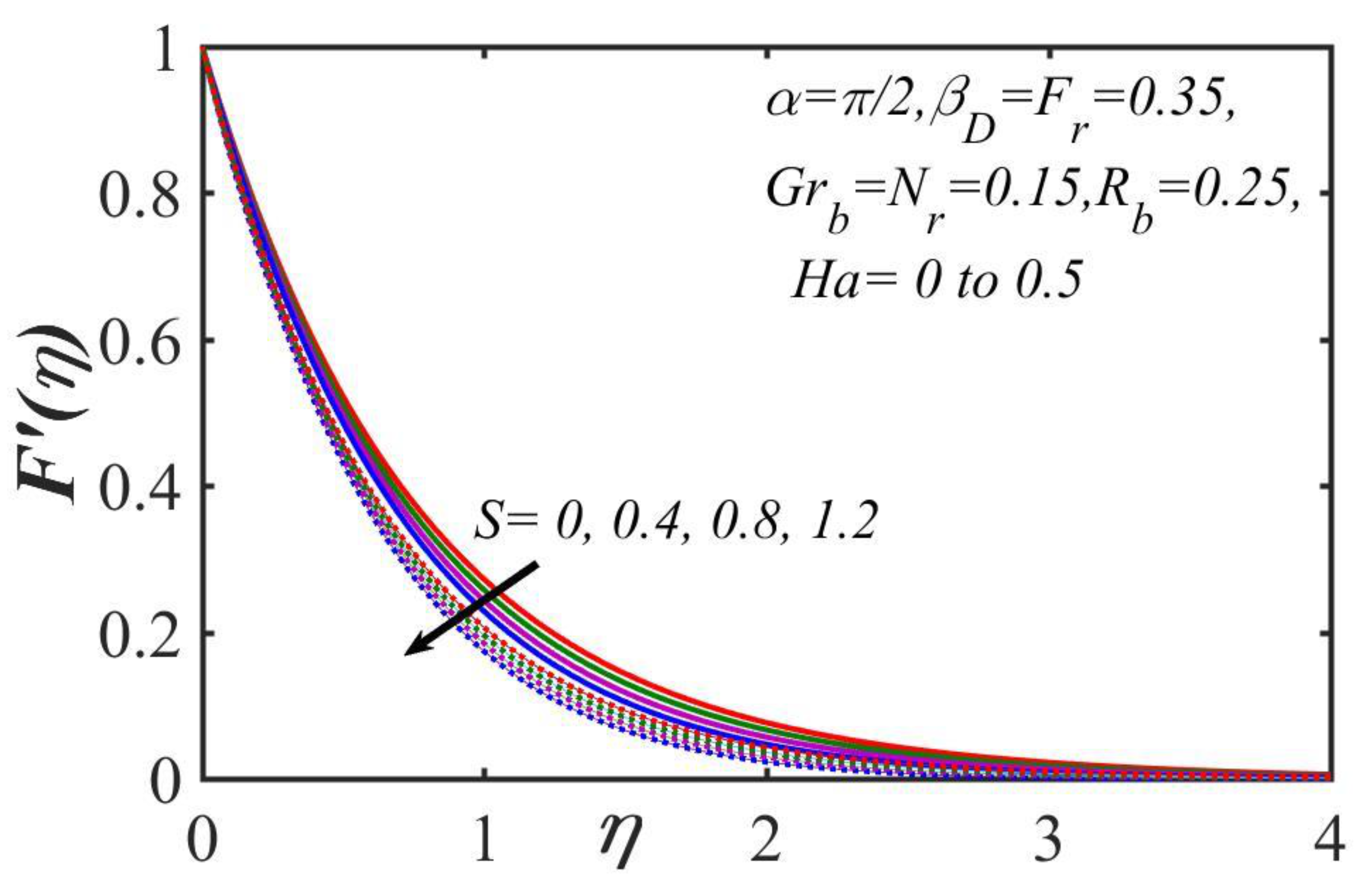
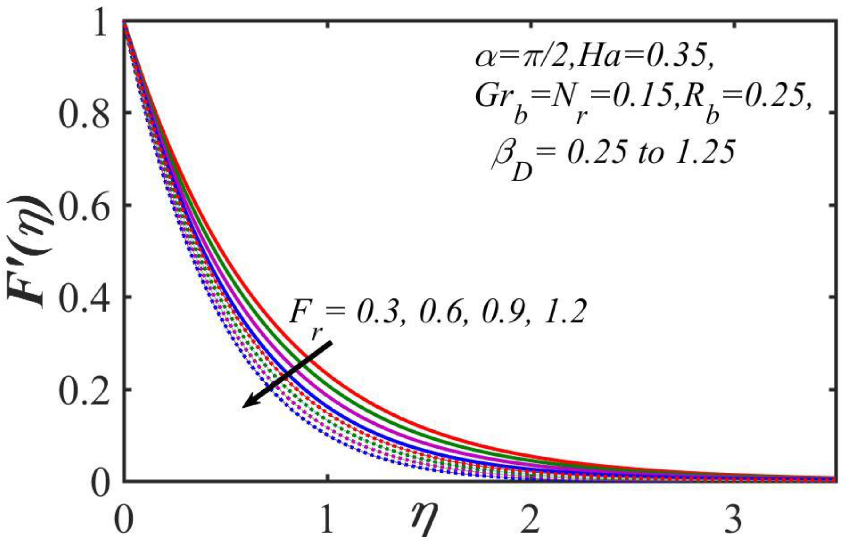
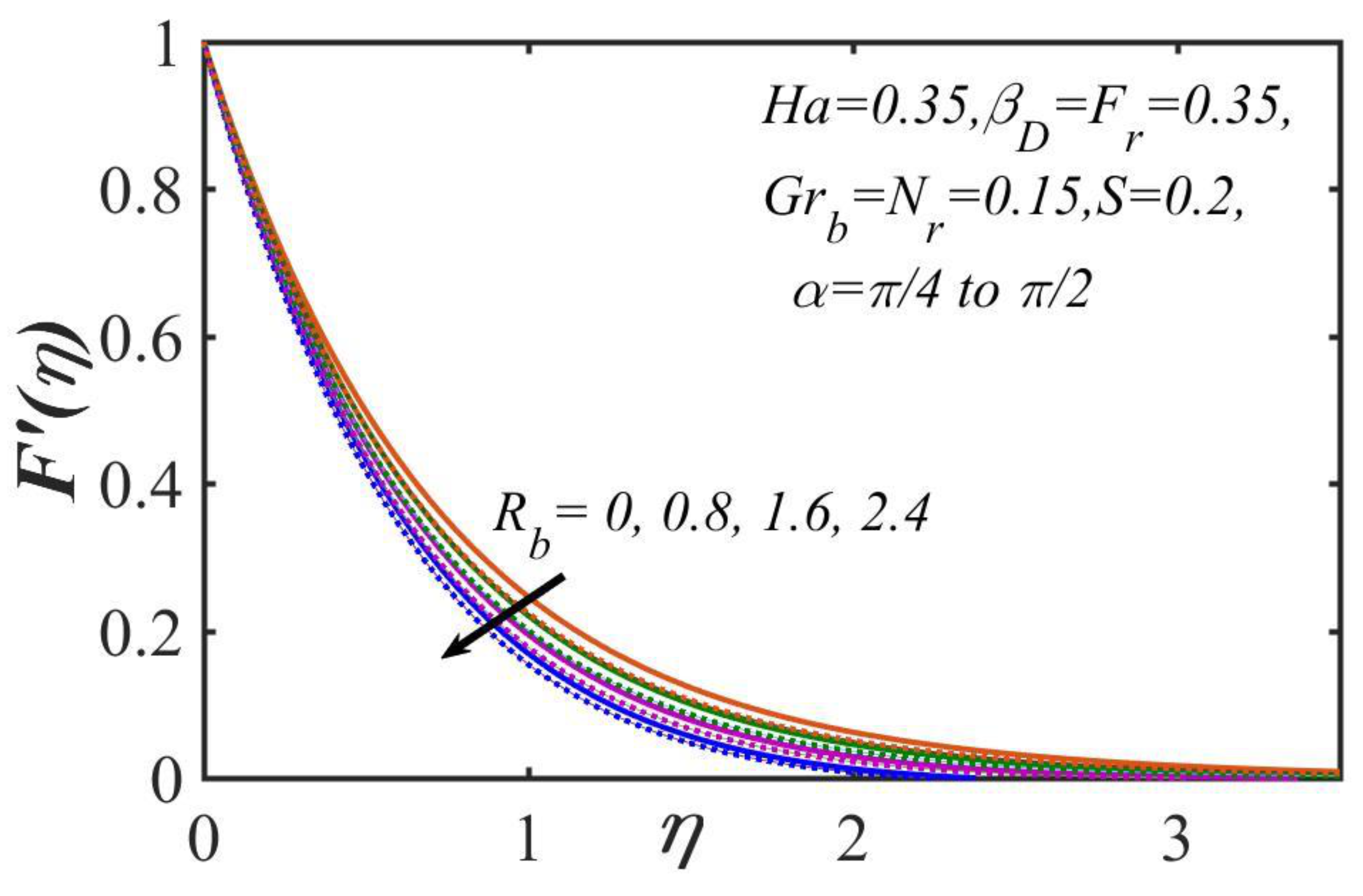
•  The velocity showed a decreasing mechanism against the higher values of the inclination angle, thermal stratification, permeability, the Darcy–Brinkman–Forchheimer parameter, the bioconvection Rayleigh number, the buoyancy proportion parameter, and the Hartmann number, as well as thickening the momentum boundary layer over the horizontal stretched surface as it reduces.
•  The velocity profiles increased as the numerical value of the mixed convection parametric quantity increased, while the thickness of the momentum boundary layer also increased.
•  The temperature magnitude decreased as the Prandtl number, the mixed convection parametric quantity, and the thermal stratification values increased; however, temperature distribution increased as the Brownian motion, Eckert number, and thermophoresis parameters increased.
•  The concentration magnitude decreased as the Lewis number and Brownian motion parameter increased, whereas they increased as the activation energy and thermophoresis parameters increased.
•  The microorganisms’ magnitudes decelerated with higher values in the bioconvection Lewis number, the motile density stratification, and the bioconvection Peclet number.
•  The SRM algorithm’s defining advantage is that it divides a large, coupled set of equations into smaller subsystems that could be handled progressively in a very computationally efficient and effective way. The proposed methodology for SRM showed that this method is accurate, easy to develop, convergent, and highly efficient in solving nonlinear problems.

References

1. Choi, S.U.; Eastman, J.A. Enhancing Thermal Conductivity of Fluids with Nanoparticles; No. ANL/MSD/CP-84938; CONF-951135-29; Argonne National Lab.: Lemont, IL, USA, 1995. [Google Scholar]
2. Das, S.K.; Choi, S.U.; Yu, W.; Pradeep, T. Nanofluids: Science and Technology; John Wiley & Sons: Hoboken, NJ, USA, 2007. [Google Scholar]
3. Buongiorno, J. Convective transport in nanofluids. J. Heat Transf. 2006, 128, 240–250. [Google Scholar] [CrossRef]
4. Tiwari, R.K.; Das, M.K. Heat transfer augmentation in a two-sided lid-driven differentially heated square cavity utilizing nanofluids. Int. J. Heat Mass Transf. 2007, 50, 2002–2018. [Google Scholar] [CrossRef]
5. Kakaç, S.; Pramuanjaroenkij, A. Review of convective heat transfer enhancement with nanofluids. Int. J. Heat Mass Transfer. 2009, 52, 3187–3196. [Google Scholar] [CrossRef]
6. Bachok, N.; Ishak, A.; Pop, I. Boundary-layer flow of nanofluids over a moving surface in a flowing fluid. Int. J. Therm. Sci. 2010, 49, 1663–1668. [Google Scholar] [CrossRef]
7. Makinde, O.D.; Aziz, A. Boundary layer flow of a nanofluid past a stretching sheet with convective boundary condition. Int. J. Therm. Sci. 2011, 50, 1326–1332. [Google Scholar] [CrossRef]
8. Haddad, Z.; Abu-Nada, E.; Oztop, H.F.; Mataoui, A. Natural convection in nanofluids: Are the thermophoresis and Brownian motion effect significant in nanofluids heat transfer enhancement. Int. J. Therm. Sci. 2012, 57, 152–162. [Google Scholar] [CrossRef]
9. Rashidi, M.M.; Nasiri, M.; Khezerloo, M.; Laraqi, N. Numerical investigation of magnetic field effect on mixed convection heat transfer of nanofluid in a channel with sinusoidal walls. J. Magn. Magn. Mater. 2016, 401, 159–168. [Google Scholar] [CrossRef]
10. Kefayati, G.H.R. Simulation of natural convection and entropy generation of non-Newtonian nanofluid in a porous cavity using Buongiorno’s mathematical model. Int. J. Heat Mass Transf. 2017, 112, 709–744. [Google Scholar] [CrossRef]
11. Ibrahim, W.; Shankar, B. MHD boundary layer flow and heat transfer of a nanofluid past a permeable stretching sheet with velocity, thermal and solutal slip boundary conditions. Comp. Fluid. 2013, 75, 1–10. [Google Scholar] [CrossRef]
12. Ibrahim, W.; Shankar, B.; Nandeppanavar, M.M. MHD stagnation point flow and heat transfer due to nanofluid towards a stretching sheet. Int. J. Heat Mass Transf. 2013, 56, 1–9. [Google Scholar] [CrossRef]
13. Mabood, F.; Khan, W.A.; Ismail, A.M. MHD boundary layer flow and heat transfer of nanofluids over a nonlinear stretching sheet: A numerical study. J. Magn. Magn. Mater. 2015, 374, 569–576. [Google Scholar] [CrossRef]
14. Khan, I.; Malik, M.Y.; Hussain, A.; Khan, M. Magnetohydrodynamics Carreau nanofluid flow over an inclined convective heated stretching cylinder with Joule heating. Results Phys. 2017, 7, 4001–4012. [Google Scholar] [CrossRef]
15. Metri, P.G.; Guariglia, E.; Silvestrov, S. Lie group analysis for MHD boundary layer flow and heat transfer over stretching sheet in presence of viscous dissipation and uniform heat source/sink. In AIP Conference Proceedings; American Institute of Physics: College Park, MA, USA, 2017; Volume 1798, p. 020096. [Google Scholar]
16. Rauf, A.; Abbas, Z.; Shehzad, S.A. Magnetohydrodynamics slip flow of a nanofluid through an oscillatory disk under porous medium supremacy. Heat Transf. Asian Res. 2019, 48, 3446–3465. [Google Scholar] [CrossRef]
17. Subhani, M.; Nadeem, S. Numerical investigation into unsteady magnetohydrodynamics flow of micropolar hybrid nanofluid in porous medium. Phys. Scr. 2019, 94, 105220. [Google Scholar] [CrossRef]
18. Zainal, N.A.; Nazar, R.; Naganthran, K.; Pop, I. Stability analysis of MHD hybrid nanofluid flow over a stretching/shrinking sheet with quadratic velocity. Alex. Eng. J. 2021, 60, 915–926. [Google Scholar] [CrossRef]
19. Singh, H.; Myong, R.S. Critical Review of Fluid Flow Physics at Micro-to Nano-scale Porous Media Applications in the Energy Sector. Adv. Mater. Sci. Eng. 2018, 2018, 9565240. [Google Scholar] [CrossRef]
20. Hassan, M.; Marin, M.; Alsharif, A.; Ellahi, R. Convective heat transfer flow of nanofluid in a porous medium over wavy surface. Phys. Lett. A 2018, 382, 2749–2753. [Google Scholar] [CrossRef]
21. Izadi, M.; Sheremet, M.A.; Mehryan, S.A.M. Natural convection of a hybrid nanofluid affected by an inclined periodic magnetic field within a porous medium. Chin. J. Phys. 2020, 65, 447–458. [Google Scholar] [CrossRef]
22. Eid, M.R.; Nafe, M.A. Thermal conductivity variation and heat generation effects on magneto-hybrid nanofluid flow in a porous medium with slip condition. Waves Random Complex Media 2020, 1–25. [Google Scholar] [CrossRef]
23. Ying, Z.; He, B.; Su, L.; Kuang, Y. Thermo-hydraulic analyses of the absorber tube with molten salt-based nanofluid and porous medium inserts. Sol. Energy 2021, 226, 20–30. [Google Scholar] [CrossRef]
24. Loganathan, K.; Alessa, N.; Tamilvanan, K.; Alshammari, F.S. Significances of Darcy–Forchheimer porous medium in third-grade nanofluid flow with entropy features. Eur. Phys. J. Spec. Top. 2021, 230, 1293–1305. [Google Scholar] [CrossRef]
25. Bees, M.A. Advances in bioconvection. Annu. Rev. Fluid Mech. 2020, 52, 449–476. [Google Scholar] [CrossRef]
26. Rashad, A.M.; Nabwey, H.A. Gyrotactic mixed bioconvection flow of a nanofluid past a circular cylinder with convective boundary condition. J. Taiwan Inst. Chem. Eng. 2019, 99, 9–17. [Google Scholar] [CrossRef]
27. Ahmad, S.; Ashraf, M.; Ali, K. Nanofluid Flow Comprising Gyrotactic Microorganisms through a Porous Medium. J. Appl. Fluid Mech. 2020, 13, 1539–1549. [Google Scholar]
28. Alshomrani, A.S. Numerical investigation for bio-convection flow of viscoelastic nanofluid with magnetic dipole and motile microorganisms. Arab. J. Sci. Eng. 2021, 46, 5945–5956. [Google Scholar] [CrossRef]
29. Habib, U.; Abdal, S.; Siddique, I.; Ali, R. A comparative study on micropolar, Williamson, Maxwell nanofluids flow due to a stretching surface in the presence of bioconvection, double diffusion and activation energy. Int. Commun. Heat Mass Transf. 2021, 127, 105551. [Google Scholar] [CrossRef]
30. Koriko, O.K.; Shah, N.A.; Saleem, S.; Chung, J.D.; Omowaye, A.J.; Oreyeni, T. Exploration of bioconvection flow of MHD thixotropic nanofluid past a vertical surface coexisting with both nanoparticles and gyrotactic microorganisms. Sci. Rep. 2021, 11, 16627. [Google Scholar] [CrossRef]
31. Bestman, A.R. Natural convection boundary layer with suction and mass transfer in a porous medium. Int. J. Energy Res. 2009, 14, 389–396. [Google Scholar] [CrossRef]
32. Makinde, O.D.; Olanrewaju, P.O.; Charles, W.M. Unsteady convection with chemical reaction and radiative heat transfer past a flat porous plate moving through a binary mixture. Afr. Mat. 2011, 22, 65–78. [Google Scholar] [CrossRef]
33. Hamid, A.; Khan, M. Impacts of binary chemical reaction with activation energy on unsteady flow of magneto-Williamson nanofluid. J. Mol. Liq. 2018, 262, 435–442. [Google Scholar] [CrossRef]
34. Irfan, M.; Khan, W.A.; Khan, M.; Gulzar, M.M. Influence of Arrhenius activation energy in chemically reactive radiative flow of 3D Carreau nanofluid with nonlinear mixed convection. J. Phys. Chem. Solids 2019, 125, 141–152. [Google Scholar] [CrossRef]
35. Zeeshan, A.; Shehzad, N.; Ellahi, R. Analysis of activation energy in Couette-Poiseuille flow of nanofluid in the presence of chemical reaction and convective boundary conditions. Results Phys. 2018, 8, 502–512. [Google Scholar] [CrossRef]
36. Zhang, L.; Bhatti, M.M.; Shahid, A.; Ellahi, R.; Bég, O.A.; Sait, S.M. Nonlinear nanofluid fluid flow under the consequences of Lorentz forces and Arrhenius kinetics through a permeable surface: A robust spectral approach. J. Taiwan Inst. Chem. Eng. 2021, 124, 98–105. [Google Scholar] [CrossRef]
37. Mosayebidorcheh, S.; Hatami, M. Analytical investigation of peristaltic nanofluid flow and heat transfer in an asymmetric wavy wall channel (Part II: Divergent channel). Int. J. Heat Mass Transf. 2018, 126, 800–808. [Google Scholar] [CrossRef]
38. Fakhar, M.H.; Fakhar, A.; Tabatabaei, H. Mathematical modeling of pipes reinforced by agglomerated CNTs conveying turbulent nanofluid and application of semi-analytical method for studying the instable Nusselt number and fluid velocity. J. Comput. Appl. Math. 2020, 378, 112945. [Google Scholar] [CrossRef]
39. Arain, M.B.; Bhatti, M.M.; Zeeshan, A.; Alzahrani, F.S. Bioconvection Reiner-Rivlin Nanofluid Flow between Rotating Circular Plates with Induced Magnetic Effects, Activation Energy and Squeezing Phenomena. Mathematics 2021, 9, 2139. [Google Scholar] [CrossRef]
40. Alsaedi, A.; Khan, M.I.; Farooq, M.; Gull, N.; Hayat, T. Magnetohydrodynamic (MHD) stratified bioconvective flow of nanofluid due to gyrotactic microorganisms. Adv. Powder Technol. 2017, 28, 288–298. [Google Scholar] [CrossRef]
41. Motsa, S.S. A new spectral relaxation method for similarity variable nonlinear boundary layer flow systems. Chem. Eng. Commun. 2013, 201, 241–256. [Google Scholar] [CrossRef]
42. Malik, M.Y.; Salahuddin, T.; Hussain, A.; Bilal, S. MHD flow of tangent hyperbolic fluid over a stretching cylinder: Using Keller box method. J. Magn. Magn. Mater. 2015, 395, 271–276. [Google Scholar] [CrossRef]
43. Fang, T.; Zhang, J.; Yao, S. Slip MHD viscous flow over a stretching sheet–an exact solution. Commun. Nonlinear Sci. Numer. Simul. 2009, 14, 3731–3737. [Google Scholar] [CrossRef]
Figure 1. Schematic flow diagram.
Mathematics 09 02514 g001
Figure 2. Variation of S and H a over velocity magnitudes. Solid curve: H a = 0 ; dotted curve: H a = 0.5 .
Mathematics 09 02514 g002
Figure 3. Variation of F r and β D on velocity magnitudes. Solid curve: β D = 0.25 ; dotted curve: β D = 1.25 .
Mathematics 09 02514 g003
Figure 4. Variation of G r and N r on velocity distribution. Solid curve: N r = 0.15 ; dotted curve: N r = 0.45 .
Mathematics 09 02514 g004
Figure 5. Effects of R b and α on velocity magnitude. Solid curve: α = π / 4 ; dotted curve: α = π / 2 .
Mathematics 09 02514 g005
Figure 6. Impact of P r and H a on temperature magnitudes. Solid curve: H a = 0 ; dotted curve: H a = 0.5 .
Mathematics 09 02514 g006
Figure 7. Impact of N t and “ N b ” on temperature magnitudes. Solid curve: N b = 0.15 ; dotted curve: N b = 1.15 .
Mathematics 09 02514 g007
Figure 8. Influence of E c and “ α ” on temperature magnitudes. Solid curve: α = π / 4 ; dotted curve: α = π / 2 .
Mathematics 09 02514 g008
Figure 9. Effects of G r and S on temperature magnitude. Hard curve: S = 0 ; dotted curve: S = 0.2 .
Mathematics 09 02514 g009
Figure 10. Impact of N t and N b on the concentration magnitudes. Solid curve: N b = 0.15 ; dotted curve: N b = 0.55 .
Mathematics 09 02514 g010
Figure 11. Influence of L e and “ Q ” on the concentration magnitudes. Solid curve: Q = 0 ; dotted curve: Q = 0.2 .
Mathematics 09 02514 g011
Figure 12. Influences of E and δ on the concentration magnitudes. Solid curve: δ = 0.55 ; dotted curve: δ = 1.1 .
Mathematics 09 02514 g012
Figure 13. Impact of ω and L e on the concentration magnitudes. Solid curve: L e = 1 ; dotted curve: L e = 1.5 .
Mathematics 09 02514 g013
Figure 14. Influence of L b and B on the microorganisms’ magnitudes. Solid curve: B = 0 ; dotted curve: B = 0.2 .
Mathematics 09 02514 g014
Figure 15. Impact of P e and Ω on the microorganisms’ magnitudes. Solid curve: Ω = 0.25 ; dotted curve: Ω = 0.75 .
Mathematics 09 02514 g015