
Comparison of Non-Newtonian Models of One-Dimensional Hemodynamics


Faculty of Applied Mathematics and Control Processes, Saint Petersburg State University, 7/9 Universitetskaya nab., 199034 Saint Petersburg, Russian
Mathematics 2021, 9(19), 2459; https://doi.org/10.3390/math9192459
Submission received: 2 September 2021
/
Revised: 25 September 2021
/
Accepted: 27 September 2021
/
Published: 2 October 2021
(This article belongs to the Special Issue Mathematics in Biomedicine)
Abstract
:The paper is devoted to the comparison of different one-dimensional models of blood flow. In such models, the non-Newtonian property of blood is considered. It is demonstrated that for the large arteries, the small parameter is observed in the models, and the perturbation method can be used for the analytical solution. In the paper, the simplified nonlinear problem for the semi-infinite vessel with constant properties is solved analytically, and the solutions for different models are compared. The effects of the flattening of the velocity profile and hematocrit value on the deviation from the Newtonian model are investigated.
1. Introduction
The one-dimensional (1D) models are used for the simulation of blood flow in large vascular systems, where the application of 2D and 3D models leads to computational difficulties [1,2,3,4]. In clinical practice, such models are used as a predictive tool in vascular surgery [5]. The 1D models are constructed by the averaging of the equations of hydrodynamics on the vessel cross-section [6,7]. The results obtained by 1D models are compatible with the averaged results of the 3D simulations [8].
As it is obtained in experiments, blood demonstrates the non-Newtonian behaviour [9], with the shear-thinning [10], thixotropic [11] and viscoelastic [12] properties. The complete 1D model of blood, with time-dependent characteristics, where all these properties are taken into account, is presented in [13]. As it is mentioned in [14], only the shear-thinning property is important for the blood flow models because the other mentioned properties do not significantly change the velocity field. The shear-thinning property of blood can be successively described by the generalized Newtonian models, where the dynamic viscosity is dependent only on the shear rate tensor [15]. For example, the models of such type are applied to the 2D and 3D blood flow simulations in [16,17,18,19,20,21].
The typical example of the generalized Newtonian fluid is a so-called Power Law model. This model is used for the 2D and 3D modelling of blood flow dynamics in a coronary artery [22], aorta [17], aorta-iliac bifurcation [23], thoracic aorta [24], carotid artery [25] and in various types of stenosed vessels [18,20,26]. In [22,27], it is demonstrated that at high shear rates, the solutions are close to the solutions for the Newtonian model, but at low shear rates, serious deviations are observed.
In many works, models with two asymptotic values of dynamic viscosity, corresponding to infinitely small and infinitely large shear rates, are used. The examples of such models are: Carreau model [9,16,17,18,19,20,22,24,27,28,29,30,31]; Carreau–Yasuda model [9,17,18,22,23,25,27,31,32,33]; Cross model [9,16,17,20,27,34,35]; Simplified Cross model [9,16,36]; Modified Cross model [9,16,22,27,36]; and Yeleswarapu model [37,38,39,40]. In [16], models of such types are applied to the simulation of blood flow in atherosclerotic coronary arteries, and results are compared with clinical measurements. The lowest average deviations are obtained for Cross and Simplified Cross models. The largest deviations are observed for the Modified Cross model. In [23], the non-Newtonian effects on the low-density lipoprotein transport in arteries are analysed. It is demonstrated that the Newtonian model is valid for mass transport at low Reynolds numbers. At high values, the non-Newtonian models provide more accurate results.
Some non-Newtonian models are dependent on the hematocrit—the typical examples are: the Quemada model, used in [16,20,27,41,42], and the Modified Yeleswarapu model [21,43].
In most works devoted to 1D models of blood flow, the non-Newtonian properties are ignored. As it is mentioned above, the complete 1D model, where the time-dependent non-Newtonian properties are considered, is proposed by Ghigo et al. [13]. Some attempts to construct the non-Newtonian models of blood flow in large vascular networks have been made in [44,45].
In the present paper, the non-Newtonian 1D models of blood flow, obtained by the averaging of Navier–Stokes equations on the vessel cross-section, are presented. It is demonstrated that for the large arteries, the small parameters take place in the models. It provides the possibility to use the perturbation method for obtaining analytical solutions of the problems for a 1D system of hemodynamical equations. The simplified but nonlinear problem for the case of a semi-infinite vessel is solved analytically. Thus, in the paper, the theoretical problem for the comparison of different 1D models is considered. The solutions obtained for the non-Newtonian models are compared with each other. The effects of the flattening of the velocity profile and hematocrit are analysed.
The paper has the following structure. In Section 2, the 1D models of blood flow are considered. The nonlinear expressions for the frictional term are presented. Section 3 is devoted to the application of the perturbation method to obtain the analytical solution of the problem for the semi-infinite interval. The solutions for the different models are compared by the values of the non-Newtonian factor, which estimates the deviations of the solutions for Newtonian and non-Newtonian models. Some concluding remarks are made in Section 4.
2. Non-Newtonian Models of One-Dimensional Hemodynamics
2.1. Non-Newtonian Models of Blood Flow
The model of blood flow as a flow of viscous incompressible fluid is described by the incompressibility condition and momentum equation, when the body force action is ignored:
where is a constant density, t is time, is the velocity, p is the pressure, is the viscous stress tensor.
The time-independent non-Newtonian model (so-called generalized Newtonian fluid) is based on the following relation [15]:
where is the strain rate tensor, is its second invariant and is a dynamic viscosity. The case of constant value of corresponds to the Newtonian fluid. The expressions for for the models, widely-used for the blood, are presented in Table 1. The value of parameter for the Newtonian model can be taken from [16,18,21,28]; values of n and k for the Power Law model can be taken from [23,46,47]; values of , , and n for the Carreau model can be taken from [9,16,17,18,19,20,21,22,23,24,48]; values of , , , n and a for the Carreau–Yasuda model can be taken from [9,16,23,33]; values of , , and m for the Cross model can be taken from [9,16,17,20,35]; values of , and for the Simplified Cross model can be taken from [9]; values of , , , m and a for the Modified Cross model can be taken from [9]; values of , and for the Yeleswarapu model can be taken from [16,38]; the dependence of these parameters on hematocrit H for the Modified Yeleswarapu model are presented in [21] and values of , , and for the Quemada model are presented in [16,20,49].
The system (1) under some assumptions (e.g., see [2,6]) can be reduced to the following form:
where are the cylindrical coordinates, is the pressure, corresponding to the vessel cross-section at coordinate z, and are the components of . System (2) can be averaged on the vessel cross-section with the following representation of [6]:
where is the mean velocity, is the vessel radius and s is the dimensionless velocity profile.
As it is demonstrated in [6,7], system (2) after the averaging is reduced to the following form:
where is the cross-sectional area, is the flow rate (), f is the frictional term, defined as [13]:
and is the momentum correction coefficient, obtained as:
where is the vessel cross-section. System (4) must be closed by the equation-of-state . For the case of flow in arteries, the following equation is widely used [8]:
where is the external pressure, and are the diastolic cross-sectional area and pressure, , where E is the Young’s modulus and h is the vessel wall thickness. The case of constant values of these parameters is considered in the present paper.
The system (4) can be rewritten using the new dimensionless variables:
where is considered as a vessel length and is estimated by the wave speed at mean pressure, . The tilde sign will be ignored in the text below.
In the dimensionless variables, system (4) is rewritten as:
where .
The expressions of for the models from Table 1 in the dimensionless case are presented in Table 2. In these expressions, the values of are used. The values of are computed from the values of , where . Thus, the system (6) will be closed if the dependence of s on y will be introduced. This expression can be obtained from the solution of the problem for the steady flow in a circular tube. For the Power Law model, this problem is solved exactly:
and is computed as:
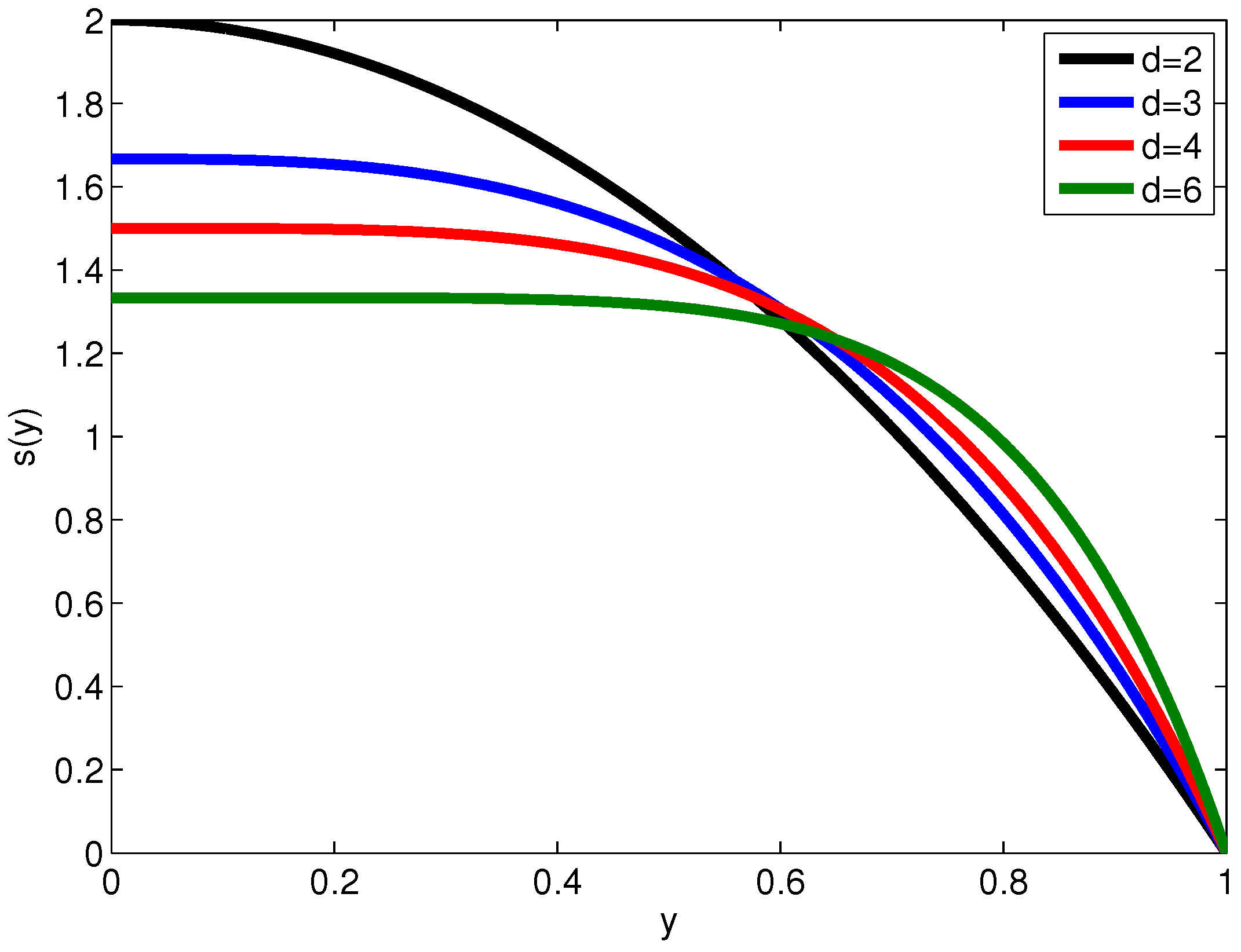
In the cases of other models, can be obtained only numerically. It can be dependent on the flow conditions (e.g., see [30,31]). According to the existence of the cellular part, the flattened velocity profile is typical for the blood [50]. Such profiles are obtained in 2D and 3D simulations of blood flow, based on the non-Newtonian models in [9,18,31,32]. For the introduction of the flattened profile by (3), into the 1D Newtonian model, in [1,4,6,7] the following expression is used:
where d is the dimensionless parameter. Plots of at various values of d are presented in Figure 1. As it can be seen, the flattening of the profile can be regulated by the proper value of d.
A similar approach is used in [13] for the time-dependent non-Newtonian 1D model, but s is dependent on t and y. The expression for the velocity profile is represented by the Womersley solution for the pulsatile flow of the Newtonian fluid in a circular tube.
Being motivated by the works mentioned above, in the presented paper we decided to use the expression (7) for the velocity profile. It must be noted that the use of the prescribed expression for the profile is a lack of the considered 1D models. However, as it is mentioned above, it is used in many other works. Moreover, as it is demonstrated in [8], the effects of a more realistic representation of the profile, where effects such as the existence of boundary layers, recirculation zones and others that can be taken into account, do not seriously change the values of the averaged characteristics. As a result, the model representation (7) is used as an approximation or simplification in this study, but parameter d will be varied to estimate the effect of profile flattening on the solution.
The value of , corresponding to (7), is computed as:
2.2. Dimensionless Parameters
For the estimation of parameters for dimensionless Equation (6), the values of , and are taken from [8] for the large arteries, such as a carotid artery, aorta and iliac artery. The value of is taken as 1.05 . The value of is estimated as 0.9783 for the carotid artery, 0.9501 for the aorta and 0.9739 for the iliac artery. Parameters , and are dependent on the parameters of rheological models and vessel properties. In the presented study, it is proposed that the following relationship between and takes place: , where is a constant.
For the Newtonian model, is approximately equal to 0.0137 for the carotid artery and ≈0.0020 for the aorta and iliac artery. For the Power Law model and parameters from [46] for the carotid artery, for aorta and for the iliac artery. For the parameters from [23,47], for carotid artery, for aorta and for iliac artery.
For the Carreau model and parameters from [9,16,17,18,20,21,22,23,24,48], is approximately equal to 15. For the dimensionless parameters, the following values take place: , for carotid artery; and for aorta; , for the iliac artery.
For the Carreau–Yasuda model and parameters from [9,16,23,33], is approximately equal to 15. The parameter has the same values as for the Carreau model. Parameter has the following values: for the carotid artery; for aorta and for iliac artery.
For the Cross model and parameters from [9], the value of is estimated as 15. Parameter has the same values as for Carreau and Carreau–Yasuda model. For , the following values take place: for the carotid artery, for aorta and 0.0084, for the iliac artery. For the parameters from [16,17,20,35] . Parameter has the same values. Parameter is equal to for the carotid artery, for aorta and for the iliac artery.
For the Simplified Cross model, is estimated as: . Parameters have the following values: , for the carotid artery; 0.0028, for aorta and 0.0029, for iliac artery.
For the case of the Modified Cross model is estimated as 25 and has the same values as for the Cross model. For the carotid artery, ; for aorta and for iliac artery.
For the Yeleswarapu model and parameters from [16,38], and as for the Simplified Cross model, for the carotid artery, 0.0028, for aorta and 0.0029, for the iliac artery.
For the Modified Yeleswarapu model, the parameters are dependent on the hematocrit H [21], so the dimensionless parameters , and are also dependent on its values. Let us obtain its values for two values of H: 0.4 and 0.5. At , the value of is approximately equal to 9.3876 and , for the carotid artery, 0.0025, for aorta and 0.0026, for iliac artery. At , the value of is estimated as 13.3797, , for the carotid artery, 0.0032, for aorta and , for iliac artery.
For the Quemada model, two parameters— and —are considered. For the parameters from [16,20,49], the following values are obtained: , for the carotid artery, , for aorta and , 25.61 for the iliac artery.
As can be seen, the small parameter is observed in the system (6), so the perturbation method can be applied to obtain analytical solutions. For most of the considered models, the large value of takes place. The first term in the expression for prevails, and if the values of are close, it can lead to the close values of the solutions for different models.
3. Solution of the Problem for the Semi-Infinite Interval
In this section, for the comparison of the models, the problem for the system (6) in the semi-infinite spatial interval is solved analytically by the perturbation method. The problem is considered as a model of the flow in a semi-infinite vessel with constant mechanical properties, which is situated at the interval . At the left side of this interval, the flow is induced by the periodic time functions, which are presented as the value of the flow rate. The perturbations induced by this function propagate at . Thus, we try to compare models on the problem, which can be solved analytically. For the solution, the assumption is used. The values of dimensionless parameters are taken for the case of the carotid artery.
It must be noted that the considered problem is analytically solved for the following purposes:
(1) To compare the results for different non-Newtonian models and estimate the deviation from the Newtonian solution;
(2) To estimate the effect of the velocity profile;
(3) To estimate the effect of hematocrit H (for the Quemada and modified Yeleswarapu models);
(4) To provide a tool for testing the programs that implement the numerical methods algorithms.
3.1. Perturbation Method
Let the semi-infinite interval be considered. The initial conditions are presented as:
where , are bounded at , , are the constants. The solutions obtained by this method correspond to the situation when the steady state, defined by the constant values and , is perturbed by the small additive terms, as shown in (8) and (9).
The boundary condition for (6) is presented as:
where are discussed below. This condition induces the flow at the left boundary .
After the substitution of (11), (12) into (6), the problems for , are formulated. In the presented study, the terms only up to and including the second order of are considered. It is easy to obtain that , .
For the first-order terms and , the following problem takes place:
where , and are defined as:
For the second-order terms , , the following problem is considered:
where
where
and constants , for every model have its own expressions. For the Power Law model (including Newtonian at ), they are written as:
For the Carreau–Yasuda model (including Carreau at ), the following expressions take place:
for the Modified Cross model ( corresponds to the Cross model, , —to the Simplified Cross model):
For the Yeleswarapu model and its modified form, and are presented as:
For the Quemada model, the following expressions are obtained:
For the simulation of the oscillatory behaviour of flow rate at , it is proposed that function in (15) is presented as:
where and are the solutions of the following initial problems:
It is easy to obtain that:
where and
at . Constants and are computed as:
Let the function be presented as:
where , , are the solutions of the following initial problems:
where ,
where .
The solution of (21) is obtained as:
where is the fundamental matrix of system . The expression for is written as: , expressions for , , , are not presented according to its cumbersomeness, but they can be easily obtained using the systems of symbolic computations.
3.2. Comparison of Solutions
For the comparison of the solutions, obtained for the non-Newtonian and Newtonian models, the following criterion, which is called the non-Newtonian factor, is used:
where norm is used, is the solution for the Newtonian model. The values of are considered in because the damping of the solution, induced by the viscosity, is most evident for this function. For various models, the following factors affect the obtained solutions: the value of and the expression for the nonlinear frictional term , which are defined by the characteristics of rheological models. These factors can lead to the difference between the solutions.
For the comparison of the solutions, the following parameter values are used: , , , t is considered on the time interval , . The plots of the real part of and corresponding for the Power Law model with parameters from [47] are presented in Figure 2. Figure 3 shows typical plots of the real parts of Q and A.
The value of for the Power Law model is equal to 2.5826 % for the parameters from [47] and to 4.4378 % for parameters from [46]. The plots of the at the midpoint of the considered space interval are presented in Figure 4. As can be seen, the strongest damping is demonstrated for the Newtonian model.
The plots of for the models without the hematocrit at different values of d are shown in Figure 5. The maximum values take place for Simplified Cross and Yeleswarapu models (≈14%) at . The maximum values for other models are realized also at this value of d and are approximately equal to 8 %. For the parabolic profile (), typical for the Newtonian model, the NNF is equal to 3 % for the Simplified Cross and Yeleswarapu model and can be considered as negligible for the other models.
In Figure 6, the plots of NNF for the models, where the value of H is included, are presented. At most H values, the value of for the parabolic profile is greater than for the Modified Yeleswarapu model, but at other d values, the situation is reversed. The greatest deviations from the solution for the Newtonian model are observed at (approximately 11% for the Quemada model and 17% for the modified Yeleswarapu model). The plots of at selected values of d and H are presented in Figure 7 in comparison with the solution for the Newtonian case.
4. Conclusions
In the presented paper, the following problems are considered:
(1) The non-Newtonian models of 1D hemodynamics are presented. Such models are constructed by the averaging of the equation of incompressible flow of viscous fluid over a vessel’s cross-section. The models are characterized by the nonlinear frictional terms, obtained from the rheological relations on the stress tensor.
(2) It is demonstrated that in the case of large arteries, small parameters are observed in the models, so the perturbation method can be used for the analytical solution of model problems.
(3) The problem for the semi-infinite space interval is solved. The expressions for the first- and second-order terms in the expansion on the small parameter are obtained.
(4) For the comparison of the solutions, the non-Newtonian factor is introduced. For the Power Law model, it is demonstrated that the flattening of the velocity profile does not lead to more significant damping of the solution than for the Newtonian case. For the other models, the deviation from the Newtonian case starts to increase with the increase in the flattening of the profile. For the models, where the hematocrit is taken into account, the deviation from the Newtonian solution increases with the increase of hematocrit value at all considered velocity profiles.
It must be noted that the obtained analytical solutions can be used for the testing of the programs, which implement the algorithms for the simulation of blood flow in large vascular systems.
The comparison of models is based on a simplified problem which can be solved analytically. For a whole comparison, the models will be compared in the cases of flows in large vascular systems, which will be considered in future works.
Funding
This research received no external funding.
Institutional Review Board Statement
Not applicable.
Informed Consent Statement
Not applicable.
Acknowledgments
The author wishes to thank the anonymous referees for careful checking of the article and helpful comments.
Conflicts of Interest
The author declares no conflict of interest.
References
- Dobroserdova, T.; Liang, F.; Panasenko, G.; Vassilevski, Y. Multiscale models of blood flow in the compliant aortic bifurcation. Appl. Math. 2019, 93, 98–104. [Google Scholar] [CrossRef]
- Quarteroni, A.; Manzoni, A.; Vergara, C. The cardiovascular system: Mathematical modelling, numerical algorithms and clinical applications. Acta Numer. 2017, 26, 365–590. [Google Scholar] [CrossRef] [Green Version]
- Boileau, E.; Nithiarasu, P.; Blanco, P.J.; Muller, L.O.; Fossan, F.E.; Hellevik, L.R.; Donders, W.P.; Huberts, W.; Willemet, M.; Alastruey, J. A benchmark study of numerical schemes for one-dimensional arterial blood flow modeling. Int. J. Numer. Methods Biomed. Eng. 2015, 31, 1–33. [Google Scholar] [CrossRef] [PubMed] [Green Version]
- Puelz, C.; Canic, S.; Riviere, B.; Rusin, C.G. Comparison of reduced models for blood flow using Runge–Kutta discontinuous Galerkin methods. Appl. Numer. Mathet. 2017, 115, 114–141. [Google Scholar] [CrossRef] [Green Version]
- Marchandise, E.; Willemet, M.; Lacroix, V. A numerical hemodynamic tool for predictive vascular surgery. Med. Eng. Phys. 2009, 31, 131–144. [Google Scholar] [CrossRef]
- Formaggia, L.; Lamponi, D.; Quarteroni, A. One-dimensional models for blood flow in arteries. J. Eng. Math. 2003, 47, 251–276. [Google Scholar] [CrossRef]
- Canic, S.; Kim, E.H. Mathematical analysis of the quasilinear effects in a hyperbolic model blood flow through compliant axi-symmetric vessels. Math. Methods Appl. Sci. 2003, 26, 1161–1186. [Google Scholar] [CrossRef]
- Xiao, N.; Alastruey, J.; Figueroa, C. A systematic comparison between 1-D and 3-D hemodynamics in compliant arterial models. Int. J. Numer. Methods Biomed. Eng. 2014, 30, 203–231. [Google Scholar] [CrossRef] [Green Version]
- Cho, Y.I.; Kensey, K.R. Effects of the non-Newtonian viscosity of blood on flows in a diseased arterial vessel. Part 1: Steady ows. Biorheology 1991, 28, 241–262. [Google Scholar] [CrossRef] [PubMed]
- Charm, S.; Kurland, G. Viscometry of human blood for shear rates of 0-100,000 sec-1. Nature 1965, 206, 617–618. [Google Scholar] [CrossRef] [PubMed]
- Huang, C.; Siskovic, N.; Robertson, R.; Fabisiak, W.; Smitherberg, E.; Copley, A. Quantitative characterization of thixotropy of whole human blood. Biorheology 1975, 12, 279–282. [Google Scholar] [CrossRef]
- Thurston, G. Viscoelasticity of human blood. Biophys. J. 1972, 12, 1205–1217. [Google Scholar] [CrossRef] [Green Version]
- Ghigo, A.R.; Lagree, P.-Y.; Fullana, J.-M. A time-dependent non-Newtonian extension of a 1D blood flow model. J. Non-Newton. Fluid Mech. 2018, 253, 36–49. [Google Scholar] [CrossRef]
- Gijsen, F.J.H.; Allanic, E.; van de Vosse, F.N.; Janssen, J.D. The influence of non-Newtonian property of blood on the flow in large arteries: Unsteady flow in a 90∘ curved tube. J. Biomech. 1999, 32, 705–713. [Google Scholar] [CrossRef]
- Irgens, F. Rheology and Non-Newtonian Fluids; Springer: Berlin, Germany, 2014. [Google Scholar]
- Abbasian, M.; Shams, M.; Valizadeh, Z.; Moshfegh, A.; Javadzadegan, A.; Cheng, S. Effects of different non-Newtonian models on unsteady blood flow hemodynamics in patient-specific arterial models with in-vivo validation. Comput. Methods Programs Biomed. 2020, 186, 105185. [Google Scholar] [CrossRef]
- Karimi, S.; Dabagh, M.; Vasava, P.; Dadvar, M.; Dabir, B.; Jalali, P. Effect of rheological models on the hemodynamics within human aorta: CFD study on CT image-based geometry. J. Non-Newton. Fluid Mech. 2014, 207, 42–52. [Google Scholar] [CrossRef]
- Razavi, A.; Shirani, E.; Sadeghi, M.R. Numerical simulation of blood pulsatile flow in a stenosed carotid artery using different rheological models. J. Biomech. 2011, 44, 2021–2030. [Google Scholar] [CrossRef] [PubMed]
- Doost, S.N.; Zhong, L.; Su, B.; Morsi, Y.S. The numerical analysis of non- Newtonian blood flow in human patient-specific left ventricle. Comput. Programs Biomed. 2016, 127, 232–247. [Google Scholar] [CrossRef]
- Molla, M.M.; Paul, M.C. LES of non-Newtonian physiological blood flow in a model of arterial stenosis. Med. Eng. Phys. 2012, 34, 1079–1087. [Google Scholar] [CrossRef] [Green Version]
- Ameenuddin, M.; Anand, M.; Massoudi, M. Effects of shear-dependent viscosity and hematocrit on blood flow. Appl. Math. Comput. 2019, 356, 299–311. [Google Scholar] [CrossRef]
- Soulis, J.V.; Giannoglou, G.D.; Chatzizisis, Y.S.; Seralidou, K.V.; Parcharidis, G.E.; Louridas, G.E. Non-Newtonian models for molecular viscosity and wall shear stress in a 3D reconstructed human left coronary artery. Med. Eng. Phys. 2008, 30, 9–19. [Google Scholar] [CrossRef] [PubMed]
- Iasiello, M.; Vafai, K.; Andreozzi, A.; Bianco, N. Analysis of non-Newtonian effects within an aorta-iliac bifurcation region. J. Biomech. 2017, 64, 153–163. [Google Scholar] [CrossRef] [PubMed]
- Caballero, A.B.; Lain, S. Numerical simulation of non-Newtonian blood flow dynamics in human thoracic aorta. Comput. Methods Biomech. Biomed. Eng. 2015, 18, 1200–1216. [Google Scholar] [CrossRef]
- Moradicheghamahi, J.; Sadeghiseraji, J.; Jahangiri, M. Numerical solution of the pulsatile, non-Newtonian and turbulent blood ow in a patient specific elastic carotid artery. Int. J. Mech. Sci. 2019, 150, 393–403. [Google Scholar] [CrossRef]
- Tu, C.; Deville, M. Pulsatile flow of non-Newtonian fluids through arterial stenoses. J. Biomech. 1996, 29, 899–908. [Google Scholar] [CrossRef]
- O’Callaghan, S.; Walsh, M.; McGloughlin, T. Numerical modelling of Newtonian and non-Newtonian representation of blood in a distal end-to-side vascular bypass graft anastomosis. Med. Eng. Phys. 2006, 28, 70–74. [Google Scholar] [CrossRef]
- Johnston, B.M.; Johnston, P.R.; Corney, S.; Kilpatrick, D. Non-Newtonian blood flow in human right coronary arteries: Steady state simulations. J. Biomech. 2004, 37, 709–720. [Google Scholar] [CrossRef] [Green Version]
- Morbiducci, U.; Gallo, D.; Massai, D.; Ponzini, R.; Deriu, M.A.; Antiga, L.; Redaelli, A.; Montevecchi, F.M. On the importance of blood rheology for bulk flow in hemodynamic models of the carotid bifurcation. J. Biomech. 2011, 44, 2427–2438. [Google Scholar] [CrossRef]
- Tabakova, S.; Nikolova, E.; Radev, S. Carreau model for oscillatory blood flow in a tube. AIP Conf. Proc. 2014, 1629, 336–343. [Google Scholar]
- Boyd, J.; Buick, J.M.; Green, S. Analysis of the Casson and Carreau–Yasuda non-Newtonian blood models in steady and oscillatory flows using the lattice Boltzmann method. Phys. Fluids 2007, 19, 093103. [Google Scholar] [CrossRef] [Green Version]
- Elhanafy, A.; Guaily, A.; Elsaid, A. Numerical simulation of blood flow in abdominal aortic aneurysms: Effects of blood shear-thinning and viscoelastic properties. Math. Comput. Simul. 2019, 160, 55–71. [Google Scholar] [CrossRef]
- Vimmir, J.; Jonasova, A. Non-Newtonian effects of blood flow in complete coronary and femoral bypasses. Math. Comput. Simul. 2010, 80, 1324–1336. [Google Scholar] [CrossRef]
- Leuprecht, A.; Perktold, K. Computer simulation of non-Newtonian effects on blood flow in large arteries. Comput. Methods Biomech. Biomed. Eng. 2001, 4, 149–163. [Google Scholar] [CrossRef] [PubMed]
- Rabby, M.G.; Razzak, A.; Molla, M.M. Pulsatile non-Newtonian blood flow through a model of arterial stenosis. Procedia Eng. 2013, 56, 225–231. [Google Scholar] [CrossRef]
- Iasiello, M.; Vafai, K.; Andreozzi, A.; Bianco, N. Analysis of non-Newtonian effects on low-density lipoprotein accumulation in an artery. J. Biomech. 2016, 49, 1437–1446. [Google Scholar] [CrossRef] [PubMed]
- Yeleswarapu, K.K.; Kameneva, M.V.; Rajagopal, K.R.; Antaki, J.F. The flow of blood in tubes: Theory and experiment. Mech. Res. Commun. 1998, 25, 257–262. [Google Scholar] [CrossRef]
- Nandakumar, N.; Sahn, K.C.; Anand, M. Pulsatile flow of a shear thinning model for blood through a two-dimensional stenosed vessel. Eur. J. Mech. 2015, 49, 29–35. [Google Scholar] [CrossRef]
- Deyranlou, A.; Niazmand, H.; Sadeghi, M.-R. Low-density lipoprotein accumulation within a carotid artery with multilayer elastic porous wall: Fluid-structure interaction and non-Newtonian considerations. J. Biomech. 2015, 48, 2948–2959. [Google Scholar] [CrossRef]
- Ameenuddin, M.; Anand, M. CFD analysis of hemodynamics in idealized abdominal aorta-renal artery junction: Preliminary study to locate atherosclerotic plague. Comput. Res. Model. 2019, 11, 695–706. [Google Scholar] [CrossRef]
- van Wyk, S.; Wittberg, L.P.; Bulusu, K.V.; Fuchs, L.; Plesniak, M.W. Non-Newtonian perspectives on pulsatile blood-analog flows in a curved artery model. Phys. Fluids 2015, 27, 071901. [Google Scholar] [CrossRef]
- Elhanafy, A.; Elsaid, A.; Guaily, A. Numerical investigation of hematocrit variation effect on blood flow in an arterial segment with variable stenosis degree. J. Mol. Liquids 2020, 313, 113550. [Google Scholar] [CrossRef]
- Wu, W.-T.; Aubry, N.; Antaki, J.F.; Massoudi, M. Simulation of blood flow in a sudden expansion channel and a coronary artery. J. Comput. Appl. Math. 2020, 376, 112856. [Google Scholar] [CrossRef]
- Perdikaris, P.; Grinberg, L.; Karniadakis, G.E. An effective fractal-tree closure model for simulating blood flow in large arterial networks. Ann. Biomed. Eng. 2015, 43, 1432–1442. [Google Scholar] [CrossRef] [PubMed] [Green Version]
- Sochi, T. The flow of power law fluids in elastic vessels and porous media. Comput. Biomech. Biomed. Eng. 2016, 19, 324–329. [Google Scholar] [CrossRef] [Green Version]
- Razavi, M.S.; Shirani, E. Development of a general methods for designing microvascular using distribution of wall shear stress. J. Biomech. 2013, 46, 2303–2309. [Google Scholar] [CrossRef]
- Kim, S.; Cho, Y.I.; Jeon, A.H.; Hogenauer, B.; Kensey, K.R. A new method for blood viscosity measurement. J. Non-Newton. Fluid Mech. 2000, 94, 47–56. [Google Scholar] [CrossRef]
- Myers, T.G. Application of non-Newtonian models to thin film flow. Phys. Rev. E 2015, 72, 066302. [Google Scholar] [CrossRef]
- Skiadopoulos, A.; Neofytou, P.; Housiadas, C. Comparison of blood rheological models in patient specific cardiovascular system simulations. J. Hydrodyn. 2017, 29, 293–304. [Google Scholar] [CrossRef]
- Caro, C.G.; Pedley, T.J.; Schroter, R.C.; Seed, W.A. The Mechanics of the Circulation; Cambridge University Press: Cambridge, UK, 2011. [Google Scholar]
Figure 1.
Plots of at different values of d.

Figure 2.
Plots of the real parts of solution on the boundary for the Power Law with parameters from [47]. (a) plot of . (b) plot of .
Figure 2.
Plots of the real parts of solution on the boundary for the Power Law with parameters from [47]. (a) plot of . (b) plot of .

Figure 3.
Plots of the real parts of solution for the Power Law with parameters from [47]. (a) plot of . (b) plot of .
Figure 3.
Plots of the real parts of solution for the Power Law with parameters from [47]. (a) plot of . (b) plot of .

Figure 4.
Plots of for the Power Law model: 1—Newtonian model; 2—model with parameters from [46]; 3—model with parameters from [47].

Figure 5.
Plots of as function of d for the models without the hematocrit: 1—Cross model with parameters from [9]; 2—Cross model with parameters from [16]; 3—Simplified Cross model; 4—Modified Cross model; 5—Carreau–Yasuda model; 6—Carreau model; 7—Yeleswarapu model.

Figure 6.
Plots of NNF for the models with hematocrit for the problem for semi-infinite interval: blue line—Modified Yeleswarapu model; red line—Quemada model.
Figure 6.
Plots of NNF for the models with hematocrit for the problem for semi-infinite interval: blue line—Modified Yeleswarapu model; red line—Quemada model.

Figure 7.
Plots of for the models including H at selected values of d and H in comparison with the solution for the Newtonian model (a) , . (b) , . Black line—Newtonian model; blue line—Modified Yeleswarapu model; red line—Quemada model.
Figure 7.
Plots of for the models including H at selected values of d and H in comparison with the solution for the Newtonian model (a) , . (b) , . Black line—Newtonian model; blue line—Modified Yeleswarapu model; red line—Quemada model.


Table 1.
Rheological models of blood as generalized Newtonian fluid.
| Model | |
|---|---|
| Newtonian | |
| Power Law | |
| Carreau | |
| Carreau–Yasuda | |
| Cross | |
| Simplified Cross | |
| Modified Cross | |
| Yeleswarapu | |
| Modified Yeleswarapu | |
| Quemada | , |
Table 2.
Expressions for the frictional term.
| Model | |
|---|---|
| Newtonian | , , , |
| Power Law | , , |
| Carreau | , |
| , , , | |
| , , | |
| Carreau–Yasuda | , |
| , , , | |
| , , | |
| Cross | , |
| , , , | |
| , , | |
| Simplified Cross | , |
| , , , | |
| , , | |
| Modified Cross | , |
| , , , | |
| , , | |
| Yeleswarapu | , |
| , , , | |
| , , | |
| Quemada | |
| , | |
| , |
Publisher’s Note: MDPI stays neutral with regard to jurisdictional claims in published maps and institutional affiliations. |
© 2021 by the author. Licensee MDPI, Basel, Switzerland. This article is an open access article distributed under the terms and conditions of the Creative Commons Attribution (CC BY) license (https://creativecommons.org/licenses/by/4.0/).
Share and Cite
MDPI and ACS Style
Krivovichev, G.V. Comparison of Non-Newtonian Models of One-Dimensional Hemodynamics. Mathematics 2021, 9, 2459. https://doi.org/10.3390/math9192459
AMA Style
Krivovichev GV. Comparison of Non-Newtonian Models of One-Dimensional Hemodynamics. Mathematics. 2021; 9(19):2459. https://doi.org/10.3390/math9192459
Chicago/Turabian StyleKrivovichev, Gerasim Vladimirovich. 2021. "Comparison of Non-Newtonian Models of One-Dimensional Hemodynamics" Mathematics 9, no. 19: 2459. https://doi.org/10.3390/math9192459
Note that from the first issue of 2016, this journal uses article numbers instead of page numbers. See further details here.