Analysis of MAP/PH/1 Queueing System with Degrading Service Rate and Phase Type Vacation

Abstract

Degradation of services arises in practice due to a variety of reasons including wear-and-tear of machinery and fatigue. In this paper, we look at $MAP/PH/1$-type queueing models in which degradation is introduced. There are several ways to incorporate degradation into a service system. Here, we model the degradation in the form of the service rate declining (i.e., the service rate decreases with the number of services offered) until the degradation is addressed. The service rate is reset to the original rate either after a fixed number of services is offered or when the server becomes idle. We look at two models. In the first, we assume that the degradation is instantaneously fixed, and in the second model, there is a random time that is needed to address the degradation issue. These models are analyzed in steady state using the classical matrix-analytic methods. Illustrative numerical examples are provided. Comparisons of both the models are drawn.

1. Introduction

It is common to see services get degraded for a variety of reasons including wear-and-tear, fatigue, and other inherent issues. Machines are the integral part of industrial systems as well as in our daily life. To address the issue of degrading service maintenance, strategies are required, and a condition-based maintenance for a single-server queueing system is analyzed by Ejaz et al. [1]. Due to the nature of offering continuous services to customers, one could expect some form of degradation to the service provided. While degradation is addressed in the context of (condition-based) maintenance in the literature (see in [1]) to the best of our knowledge the degradation of services in the context of a more general queueing model has not been addressed so far. queueing models play an important role in the study of service systems. In this paper, we incorporate the degradation of services in the context of a single server, Markovian arrival process ($MAP$), and phase type ($PH-$) services. We look at two models. In the first model, we assume that the degradation is instantaneously fixed, and in the second model, there is a random time that is needed to address the degradation issue. This random duration can be thought of as a maintenance time or a vacation time during which the degradation issues are addressed and fixed.

When instantaneous fixing (such as new server/machine replacing the existing one) of the degrading issues is not possible, it is natural to introduce a random duration to address such issues. queueing models where there is a discontinuity in providing services have been studied under the theme of queueing systems with vacations. Such models have been studied extensively in the literature. We refer to the survey paper by Doshi [2] and the book by Tian and Zhang [3] for vacation queueing models. A working vacation means that the server works with a lower service rate than the normal rate provided during the busy period of the server. This type of working vacation model was introduced by Servi and Finn [4]. Kim et al. [5] generalized the working vacation concept for $M/G/1$ queue and analyzed the queue length distribution in steady state. Multiple working vacations were studied by Baba [6] for the $GI/M/1$ queueing system. Li and Tian [7] studied the working vacation for the $M/M/1$ model and introduced the vacation interruption in which due to some conditions the server will be back without completing the ongoing vacation. In the context of a multiple server queueing system, Chakravarthy [8,9] studied the synchronous vacations and phase type distributed vacation periods. He discussed an optimization problem and did the steady-state analysis of the model. A survey emphasizing on the matrix-analytic method and the working vacation in the queueing models is presented in Tian et al. [10]. Working vacations and vacation interruptions in the context of an $MAP/G/1$ model were studied by Zhang and Hou [11]. Using supplementary method and matrix-analytic method, they obtained the queue length distribution in steady state. In [12,13], Chakravarthy studied queueing models in which vacations and optional secondary services were used. Sreenivasan et al. [14] studied queueing models with $MAP$ arrivals, phase type services and with working vacations, N-policy, and vacation interruptions. The vacation is interrupted whenever the number of customers in the queue reaches a threshold number N. Alfa [15] studied vacations for the $MAP/PH/1$ model using the classical matrix-analytic method and established decomposition results for the rate matrices R and G. He extended his theory to $BMAP/PH/1$ queues, and also showed the results for the models $G\mathit{e}o/PH/1$ and $M/PH/1$. Cost optimization in the context of $M/M/1$ queueing model was analyzed by Yang and Wu [16] considering the vacation of the server and the server breakdown. The vacation of the server is also interrupted when the number of customers reaches a predetermined threshold. The concept of a back-up server (during the times the main server is under repair) serving at a lower rate, in the context of $MAP/PH/1$ queueing model was analyzed by Chakravarthy et al. [17]. Recently, Jain et al. [18] analyzed the working vacation queue with imperfect service and impatient customers. Using the simulation approach, Chakravarthy [19] did a comparative study of the queueing models with various vacation policies and obtained some interesting results.

In this study, we incorporate the degradation of services in the context of $MAP/PH/1$-type queues. The organization of the paper is as follows. In Section 2, we analyze the first model in steady state including establishing the stability condition and list some key performance measures. In Section 3, the second model is explained along with the stability condition, the steady-state solutions, and key performance measures. In Section 4, we discuss a few illustrative numerical examples. Concluding remarks are provided in Section 5.

In the sequel, we set the following notations.

• All bold-faced letters will indicate either row or column vectors which will be clear from context.
• e is the column vector with 1’s, of appropriate dimension. Where clarifications on the dimensions are needed, we will indicate accordingly.
• ${\mathit{e}}_i\left(m\right)$ is a column vector of dimension m with all but one entries are zero and the nonzero entry in the ith position is taken to be 1. That is, ${\mathit{e}}_i\left(m\right)={\left(\begin{array}{ccccc}0& \cdots & 1& \cdots & 0\end{array}\right)}^t,$ where the notation ‘t’ denotes the transpose notation.
• I is the identity matrix of appropriate order.
• The symbols ⊗ and ⊕ stand for the Kronecker product and the Kronecker sum, respectively. Note that these play a major role in stochastic modeling. For more information, one can refer to the works in [20,21].

2. $\mathit{MAP}/\mathit{PH}/\mathbf{1}$ Model with Degradation Restored Instantaneously ($\mathit{Model}\mathbf{1}$)

We assume that the customers arrive according to a Markovian arrival process ($MAP$) which was introduced by Neuts [22] in a more general context. Modeling of the customers’ arrivals with $MAP$ is very useful and natural in the context of both independent and correlated nature of the arrival processes. Let $D=D_0+D_1$ be the generator of $MAP$, where $D_0$ governs transitions for no arrival, whereas $D_1$ governs transitions for an arrival in the system, and both $D_0$ and $D_1$ are of dimension m. If $\mathit{\pi }$ denotes the stationary vector of D, then we have

$$\mathit{\pi }D=0,\mathrm{and}\mathit{\pi }\mathit{e}=1.$$

The arrival rate is then given by, $\lambda =\mathit{\pi }{D}_1\mathit{e}$.

The system is studied on a first-come-first-served ($FCFS$) basis. The service times are modeled using $PH$-distribution, which was introduced by Neuts [23]. We assume that the $PH$-distribution has an irreducible representation given by $(\mathit{\beta },S)$ of order n. The average service rate, $\mu$, is given by $\mu ={\left[\mathit{\beta }{(-S)}^{-1}\mathit{e}\right]}^{-1}$. For more details on $PH$-distributions and $MAP$, we refer the reader to the works in [24,25,26,27,28,29] and the recent book by Dudin et al. [30].

The service rate degrades after completion of each service. Let the initial service rate be $\mu$ and the service rate of the ith service be ${\mu }_i$ such that $\mu ={\mu }_1\ge {\mu }_2\ge {\mu }_3\ge \cdots \ge {\mu }_L,$ where ${\mu }_i={\theta }_i\mu$, and $0<{\theta }_i\le 1$, for all $i=1,2,3,\cdots ,L$. The degraded service rate is restored to the original rate of $\mu$ instantaneously after completion of L services or whenever the server becomes idle. Note that ${\theta }_1=1$ so that the service rate of the first customer after addressing the degradation is always $\mu$.

2.1. Generator of the Model

At any time t, we define the following random variables so as to keep track of the status of the system.

• $N_1\left(t\right)$ is the number of customers in the system,
• $N_2\left(t\right)$ is the phase of service, if any,
• $N_3\left(t\right)$ is the phase of arrival process.
• $N_4\left(t\right)$ is the type of service, if any.

Therefore, $\{(N_1\left(t\right),N_2\left(t\right),N_3\left(t\right),N_4\left(t\right)),t\ge 0\}$ forms a Markov process on state space: $\mathsf{\Omega }=\left\{\right(0,k):1\le k\le m\}\cup \left\{\right(i,j,k,l):1\le j\le n,1\le k\le m,1\le l\le L,i\ge 1\}$. Define $\mathit{\theta }={({\theta }_1,{\theta }_2,\cdots ,{\theta }_L)}^t,$ and $\mathsf{\Delta }\left(\mathit{\theta }\right)=\left(\begin{array}{c}{\theta }_1\\ & {\theta }_2\\ & & \ddots \\ & & & {\theta }_L\end{array}\right)$. Then, the generator governing the system under study is given by

$$Q^{\left(1\right)}=\left(\begin{array}{ccccc}{D}_0& {\mathit{e}}_{\mathbf{1}}^{\mathit{\prime }}\otimes \mathit{\beta }\otimes D_1& 0& 0& \cdots \\ \mathit{\theta }\otimes S^0\otimes I& A_1& A_0& 0& \cdots \\ 0& A_2& A_1& A_0& \cdots \\ ⋮& \ddots & \ddots & & \ddots \end{array}\right),$$

where

$$A_0=I\otimes D_1,A_1=(\mathsf{\Delta }\left(\mathit{\theta }\right)\otimes S)\oplus D_0,$$

and

$$A_2=\left(\begin{array}{ccccc}0& {\theta }_1{S}^0\mathit{\beta }\otimes I& 0& \cdots & 0\\ 0& 0& {\theta }_2{S}^0\mathit{\beta }\otimes I& \cdots & 0\\ ⋮& ⋮& ⋮& \ddots & ⋮\\ 0& 0& 0& \cdots & {\theta }_{L-1}{S}^0\mathit{\beta }\otimes I\\ {\theta }_L{S}^0\mathit{\beta }\otimes I& 0& 0& \cdots & 0\end{array}\right).$$

Note that $A_0,A_1$, and $A_2$ are square matrices of order $Lmn$. The dimensions of the other matrices appearing in $Q^{\left(1\right)}$ should be self-explanatory.

2.2. Stability Analysis

Here, we will derive the stability condition in terms of the input parameters.

Result 1.

The queueing system, namely, Model 1, under study is stable if and only if

$$\lambda <\mu L{\left[\sum _{j=1}^L\frac{1}{{\theta }_j}\right]}^{-1}.$$

(1)

Proof. 

Letting $A=A_0+A_1+A_2$, we get

$$A=\left(\begin{array}{ccccc}{\theta }_{1}S\oplus D& {\theta }_1{S}^0\mathit{\beta }\otimes I& 0& \cdots & 0\\ 0& {\theta }_{2}S\oplus D& {\theta }_2{S}^0\mathit{\beta }\otimes I& \cdots & 0\\ ⋮& \ddots & \ddots & \ddots & ⋮\\ 0& 0& 0& \cdots & {\theta }_{L-1}{S}^0\mathit{\beta }\otimes I\\ {\theta }_L{S}^0\mathit{\beta }\otimes I& 0& 0& \cdots & {\theta }_{L}S\oplus D\end{array}\right).$$

Define, $\mathit{\delta }=({\mathit{\delta }}_{\mathbf{1}},{\mathit{\delta }}_{\mathbf{2}},\cdots ,{\mathit{\delta }}_L)$ with ${\mathit{\delta }}_j,1\le j\le L,$ of dimension $1\times mn$ to be the steady-state probability vector of the matrix A. Then, $\mathit{\delta }A=0,\mathrm{and}\mathit{\delta }\mathit{e}=1$. Therefore,

$$\begin{array}{cc}\hfill {\mathit{\delta }}_1({\theta }_{1}S\oplus D)+{\mathit{\delta }}_L({\theta }_L{S}^0\mathit{\beta }\otimes I)& =\mathbf{0},\hfill \\ \hfill {\mathit{\delta }}_{j-1}({\theta }_{j-1}{S}^0\mathit{\beta }\otimes I)+{\mathit{\delta }}_j({\theta }_{j}S\oplus D)& =\mathbf{0},2\le j\le L-1,\hfill \\ \hfill {\mathit{\delta }}_{L-1}({\theta }_{L-1}{S}^0\mathit{\beta }\otimes I)+{\mathit{\delta }}_L({\theta }_{L}S\oplus D)& =\mathbf{0},\hfill \end{array}$$

(2)

with

$$\sum _{j=1}^L{\mathit{\delta }}_j\mathit{e}=1.$$

(3)

Summing up the equations in (2) over j, we get

$$\sum _{j=1}^L{\mathit{\delta }}_{\mathit{j}}\left[({\theta }_{j}S+{\theta }_j{S}^0\mathit{\beta })\oplus D\right]=\mathbf{0}.$$

Using the uniqueness of the invariant vector $\mu \mathit{\beta }{(-S)}^{-1}$ of the generator ($S+S^0\mathit{\beta }$), along with the fact that, if b and c are the invariant vectors of B and C, then $b\otimes c$ is the invariant vector of $B\oplus C$, we get

$${\mathit{\delta }}_{\mathit{j}}=\frac{d}{{\theta }_j}(\mathit{\beta }{(-S)}^{-1}\otimes \mathit{\pi }),$$

(4)

where d is the normalizing constant to satisfy Equation (3) and is given by

$$d=\mu {\left[\sum _{j=1}^L\frac{1}{{\theta }_j}\right]}^{-1}.$$

(5)

As the above model is a quasi-birth-and-death ($QBD$) model, the stability condition for this model is given by $\mathit{\delta }{A}_0\mathit{e}<\mathit{\delta }{A}_2\mathit{e}$ (see in [31]),

$$\begin{array}{c}\hfill \lambda <\sum _{j=1}^L{\theta }_j{\mathit{\delta }}_j(S^0\otimes \mathit{e}),\\ \hfill \Rightarrow \lambda <\mu L{\left[\sum _{j=1}^L\frac{1}{{\theta }_j}\right]}^{-1}.\end{array}$$

□

Remark 1.

When ${\theta }_j=1$ for all $j,1\le j\le L$, then the stability condition reduces to that of the corresponding classical queueing model, that is, $\lambda <\mu$. This is due to the fact that in Model 1 the server remains available after becoming idle to serve at the normal rate of μ.

2.3. Steady-State Probability Vector

Assuming that the stability condition given in Equation (1) holds good, the steady-state probability vector of $Q^{\left(1\right)}$ exists. Let $\mathit{x}=({\mathit{x}}_0,{\mathit{x}}_1,\cdots )$ be the steady-state probability vector such that

$$\mathit{x}{Q}^{\left(1\right)}=0,\mathrm{and}\mathit{x}\mathit{e}=1.$$

Then, due to the nature of $Q^{\left(1\right)}$, which is a $QBD$-process, the steady-state probabilities are (see in [31]) obtained as

$${\mathit{x}}_i={\mathit{x}}_1{R}^{i-1},i\ge 1,$$

where ${\mathit{x}}_0$ and ${\mathit{x}}_1$ are obtained by solving

$$\begin{array}{cc}\hfill {\mathit{x}}_0{D}_0+{\mathit{x}}_1(\mathit{\theta }\otimes S^0\otimes I)& =\mathbf{0},\hfill \\ \hfill {\mathit{x}}_0({{\mathit{e}}^{\mathit{\prime }}}_1\otimes \mathit{\beta }\otimes D_1)+{\mathit{x}}_1(A_1+R{A}_2)& =\mathbf{0},\hfill \\ \hfill {\mathit{x}}_0\mathit{e}+{\mathit{x}}_1{(I-R)}^{-1}\mathit{e}& =1,\hfill \end{array}$$

(6)

and the rate matrix R is the minimal non-negative solution to the matrix-quadratic equation $R^2{A}_2+R{A}_1+A_0=0.$

2.4. Performance Measures

For the qualitative study of the model, we look at the following key system performance measures.

• Mean number of the customers in the system $L_s={\sum }_{i=1}^{\infty }i{\mathit{x}}_i\mathit{e}={\mathit{x}}_1{(I-R)}^{-2}\mathit{e}.$
• Mean waiting time of the customer in the system $W_s=\frac{L_s}{\lambda }$.
• Probability of the server being in busy state $P_{busy}={\sum }_{i=1}^{\infty }{\mathit{x}}_i\mathit{e}$.
• Probability of the server being in idle state $P_{idl\mathit{e}}={\mathit{x}}_0\mathit{e}$.

3. $\mathit{MAP}/\mathit{PH}/\mathbf{1}$ Model with Degradation Restored after a Random Time (a.k.a. Vacation)—$\mathit{Model}\mathbf{2}$

In this model, the degraded system is restored to a normal one after a random time. This random time is referred to as a vacation time for the server. Like in Model 1, the system is restored to a normal one either when the server becomes idle or after L service completions. However, here the restoration time is random. We will henceforth refer to this as vacation time. Note that once the random time expires, the server returns and at that time the system is restored to its original state. One can view this as the server is recalled at the instant of the restoration of the system. We assume that the vacation time follows a $PH$-distribution with an irreducible representation given by ${(\mathit{r},V)}_{\nu }.$ Let ${\mathit{V}}^{\mathbf{0}}$ be such that $V\mathit{e}+{\mathit{V}}^{\mathbf{0}}=0$ and $\tilde{V}=V+{\mathit{V}}^{\mathbf{0}}\mathit{r}$. Then, the average vacation rate ${\mu }_{\nu }={\left[\mathit{r}{(-V)}^{-1}\mathit{e}\right]}^{-1}.$ The arrivals and the services are according to $MAP$ and $PH$-type, respectively, same as considered for the previous model. All the processes considered in this model are mutually independent.

3.1. Generator of the Model

Let us define the random variables, at any time t as,

• $N_1\left(t\right)$ is the number of customers in the system,
• $N_2\left(t\right)$ is the phase of vacation or service depending on the server being idle or busy,
• $N_3\left(t\right)$ is the phase of arrival process,
• $N_4\left(t\right)$ is the type of service when the server is busy.

Then, $\{(N_1\left(t\right),N_2\left(t\right),N_3\left(t\right),N_4\left(t\right)),t\ge 0\}$ forms a Markov process on the state space, $\mathsf{\Omega }=\left\{\mathbf{0}\right\}\cup \left\{\mathit{i}\right\}$, where $\mathbf{0}=\{(0,j_1,k):1\le j_1\le \nu ,1\le k\le m\}$, and $\mathit{i}=\{(i,j_2,k,l):1\le j_2\le n,1\le k\le m,1\le l\le L\}\cup \{(i,j_1,k):1\le j_1\le \nu ,1\le k\le m\},i\ge 1.$

Therefore, the generator of the system governing Model 2 is given by

$$Q^{\left(2\right)}=\left(\begin{array}{ccccc}\tilde{V}\oplus D_0& B_1& 0& 0& \cdots \\ \mathit{\theta }\otimes S^0\mathit{r}\otimes I& {A_1}^{\left(v\right)}& {A_0}^{\left(v\right)}& 0& \cdots \\ 0& {A_2}^{\left(v\right)}& {A_1}^{\left(v\right)}& {A_0}^{\left(v\right)}& \cdots \\ ⋮& \ddots & \ddots & & \ddots \end{array}\right),$$

where

$$B_1=(O,I\otimes D_1),{A_0}^{\left(v\right)}=I\otimes D_1,$$

$${A_1}^{\left(v\right)}=\left(\begin{array}{cc}{A}_1& O\\ {\mathit{e}}_1^{\mathit{\prime }}\left(L\right)\otimes {\mathit{V}}^{\mathbf{0}}\mathit{\beta }\otimes I& V\oplus D_0\end{array}\right),{A_2}^{\left(v\right)}=\left(\begin{array}{cc}{\widehat{A}}_2& {\mathit{e}}_L\otimes {\theta }_L{S}^0\mathit{r}\otimes I\\ O& O\end{array}\right),$$

and ${\widehat{A}}_2=\left(\begin{array}{ccccc}0& {\theta }_1{S}^0\mathit{\beta }\otimes I& 0& \cdots & 0\\ 0& 0& {\theta }_2{S}^0\mathit{\beta }\otimes I& \cdots & 0\\ ⋮& ⋮& ⋮& \ddots & ⋮\\ 0& 0& 0& \cdots & {\theta }_{L-1}{S}^0\mathit{\beta }\otimes I\\ 0& 0& 0& \cdots & 0\end{array}\right)$.

3.2. Stability Analysis

Result 2.

The system governing Model 2 is stable if and only if

$$\lambda <L{\left[\frac{1}{\mu }\sum _{j=1}^L\frac{1}{{\theta }_j}+(\mathit{r}\otimes \mathit{\pi })(-{(V\oplus D)}^{-1})\mathit{e}\right]}^{-1}.$$

(7)

Proof. 

Let the invariant probability vector ${\mathit{\delta }}^{\left(v\right)}=({\mathit{\delta }}_1^{\left(v\right)},{\mathit{\delta }}_2^{\left(v\right)},\cdots ,{\mathit{\delta }}_L^{\left(v\right)},{\mathit{\delta }}^{\ast })$ of $A^{\left(v\right)}=A_0^{\left(v\right)}+A_1^{\left(v\right)}+A_2^{\left(v\right)}$ be such that

$${\mathit{\delta }}^{\left(v\right)}{A}^{\left(v\right)}=\mathbf{0},\mathrm{and}{\mathit{\delta }}^{\left(v\right)}\mathit{e}=1.$$

Then, we have

$$\begin{array}{ccc}\hfill {\mathit{\delta }}_1^{\left(v\right)}({\theta }_{1}S\oplus D)+{\mathit{\delta }}^{\ast }({\mathit{V}}^{\mathbf{0}}\mathit{\beta }\otimes I)& =& \mathbf{0},\hfill \end{array}$$

(8)

$$\begin{array}{ccc}\hfill {\mathit{\delta }}_{j-1}^{\left(v\right)}({\theta }_{j-1}{S}^0\mathit{\beta }\otimes I)+{\mathit{\delta }}_j^{\left(v\right)}({\theta }_{j}S\oplus D)& =& \mathbf{0},2\le j\le L,\hfill \end{array}$$

(9)

$$\begin{array}{ccc}\hfill {\mathit{\delta }}^{\ast }(V\oplus D)+{\mathit{\delta }}_L^{\left(v\right)}({\theta }_L{S}^0\mathit{r}\otimes I)& =& \mathbf{0}.\hfill \end{array}$$

(10)

Using Equation (10), we get

$${\mathit{\delta }}^{\ast }={\mathit{\delta }}_L^{\left(v\right)}({\theta }_L{S}^0\mathit{r}\otimes I)(-{(V\oplus D)}^{-1}).$$

Now, after multiplying Equation (10) by $(\mathit{e}\mathit{\beta }\otimes I)$, we get

$$-{\mathit{\delta }}^{\ast }({\mathit{V}}^{\mathbf{0}}\mathit{\beta }\otimes I)+{\mathit{\delta }}^{\ast }(\mathit{e}\mathit{\beta }\otimes D)+{\mathit{\delta }}_L^{\left(v\right)}({\theta }_L{S}^0\mathit{\beta }\otimes I)=0.$$

(11)

Substituting (11) in (8) and adding the resulting equation to Equation (10) and the one obtained by summing over $1\le j\le L,$ of those equations in (9), we get

$$\sum _{j=1}^L{\mathit{\delta }}_j^{\left(v\right)}\left[({\theta }_{j}S+{\theta }_j{S}^0\mathit{\beta })\oplus D\right]+{\mathit{\delta }}^{\ast }(\mathit{e}\mathit{\beta }\otimes D)=0.$$

(12)

Furthermore, we have

$$\sum _{j=1}^L{\mathit{\delta }}_j^{\left(v\right)}(\mathit{e}\otimes I)+{\mathit{\delta }}^{\ast }(\mathit{e}\otimes I)=\mathit{\pi }.$$

(13)

Now, after multiplying Equation (13) by $(\mathit{e}\mathit{\beta }\otimes D)$, we get

$$\sum _{j=1}^L{\mathit{\delta }}_j^{\left(v\right)}(\mathit{e}\mathit{\beta }\otimes D)+{\mathit{\delta }}^{\ast }(\mathit{e}\mathit{\beta }\otimes D)=\mathbf{0}.$$

(14)

Now, using ${\mathit{\delta }}_j^{\left(v\right)}(\mathit{e}\mathit{\beta }\otimes D)=0,\forall j$, we get

$${\mathit{\delta }}^{\ast }(\mathit{e}\mathit{\beta }\otimes D)=\mathbf{0}.$$

(15)

Then, from Equation (12), we get

$${\mathit{\delta }}_j^{\left(v\right)}=\frac{d}{{\theta }_j}(\mathit{\beta }{(-S)}^{-1}\otimes \mathit{\pi })\mathrm{and}{\mathit{\delta }}^{\ast }(\mathit{e}\mathit{\beta }\otimes D)=\mathbf{0},$$

where d is the normalizing constant appearing in the following equation:

$$d\left[\frac{1}{\mu }\sum _1^L\frac{1}{{\theta }_j}+(\mathit{r}\otimes \mathit{\pi })(-{(V\oplus D)}^{-1})\mathit{e}\right]=1.$$

(16)

Now using the stability condition ${\mathit{\delta }}^{\left(v\right)}{A}_0^{\left(v\right)}\mathit{e}<{\mathit{\delta }}^{\left(v\right)}{A}_2^{\left(v\right)}\mathit{e}$, we get

$$\begin{array}{cc}\hfill \lambda & <\sum _{j=1}^L{\theta }_j{\mathit{\delta }}_j^{\left(v\right)}(S^0\otimes \mathit{e}),\hfill \\ \hfill \Rightarrow \lambda & <L{\left[\frac{1}{\mu }\sum _{j=1}^L\frac{1}{{\theta }_j}+(\mathit{r}\otimes \mathit{\pi })(-{(V\oplus D)}^{-1})\mathit{e}\right]}^{-1}.\hfill \end{array}$$

□

3.3. Steady-State Probability Vector

The stability condition (7) ensures that the steady-state probability vector exists for the current model. Let ${\mathit{x}}^{\left(v\right)}=({\mathit{x}}_0^{\left(v\right)},{\mathit{x}}_1^{\left(v\right)},\cdots )$ be the steady-state probability vector such that ${\mathit{x}}^{\left(v\right)}{Q}^{\left(2\right)}=0,$ and ${\mathit{x}}^{\left(v\right)}\mathit{e}=1.$

Then, applying Neuts’ result on QBD-process, we get

$${\mathit{x}}_i^{\left(v\right)}={\mathit{x}}_1^{\left(v\right)}{R}_v^{i-1},i\ge 1,$$

where ${\mathit{x}}_0^{\left(v\right)}$ and ${\mathit{x}}_1^{\left(v\right)}$ are obtained by solving

$$\begin{array}{cc}\hfill {\mathit{x}}_0^{\left(v\right)}(\tilde{V}\oplus D_0)+{\mathit{x}}_1^{\left(v\right)}(\mathit{\theta }\otimes S^0\mathit{r}\otimes I)& =\mathbf{0},\hfill \\ \hfill {\mathit{x}}_0^{\left(v\right)}{B}_1+{\mathit{x}}_1^{\left(v\right)}(A_1^{\left(v\right)}+R_v{A}_2^{\left(v\right)})& =\mathbf{0},\hfill \\ \hfill {\mathit{x}}_0^{\left(v\right)}\mathit{e}+{\mathit{x}}_1^{\left(v\right)}{(I-R_v)}^{-1}\mathit{e}& =1.\hfill \end{array}$$

(17)

and $R_v$ is the minimal nonnegative solution to $R_v^2{A}_2^{\left(v\right)}+R_v{A}_1^{\left(v\right)}+A_0^{\left(v\right)}=0.$

3.4. Performance Measures

Following are the performance measures for the model under study in this section.

• Mean number of customers in the system $L_s^{\left(v\right)}={\sum }_{i=1}^{\infty }i{\mathit{x}}_i^{\left(v\right)}\mathit{e}={\mathit{x}}_1^{\left(v\right)}{(I-R_v)}^{-2}\mathit{e}.$
• Mean waiting time of the customer in the system $W_s^{\left(v\right)}=\frac{L_s^{\left(v\right)}}{\lambda }.$
• Probability of the server being in busy state $P_{busy}={\sum }_{i=1}^{\infty }{\mathit{x}}_i^{\left(v\right)}\left(\begin{array}{c}\mathit{e}\\ \mathbf{0}\end{array}\right).$

• (a)

  Probability of the server being on vacation with no customer in the system $P_{NCvacation}={\mathit{x}}_0^{\left(v\right)}\mathit{e}.$

  (b)

  Probability of the server being on vacation with at least one customer in the system $P_{OCvacation}={\sum }_{i=1}^{\infty }{\mathit{x}}_i^{\left(v\right)}\left(\begin{array}{c}0\\ \mathit{e}\end{array}\right).$

  (c)

  Probability of the server being on vacation $P_{vacation}={\mathit{x}}_0^{\left(v\right)}\mathit{e}+{\sum }_{i=1}^{\infty }{\mathit{x}}_i^{\left(v\right)}\left(\begin{array}{c}0\\ \mathit{e}\end{array}\right).$

4. Numerical Examples

In this section, we will discuss a few illustrative numerical examples of the two models under study in this paper. For the arrival process, we include five different $MAP$ processes as Erlang, exponential, hyperexponential, negatively correlated, and positively correlated arrivals having independent and identical distribution of inter-arrival times.

Notations for all the arrival processes are fixed as follows.

(i)

$ErA$—This is the Erlang distribution of order 5 for the arrival process. Here

• $D_0=\left(\begin{array}{ccccc}-5& 5& 0& 0& 0\\ 0& -5& 5& 0& 0\\ 0& 0& -5& 5& 0\\ 0& 0& 0& -5& 5\\ 0& 0& 0& 0& -5\end{array}\right)$ and $D_1=\left(\begin{array}{ccccc}0& 0& 0& 0& 0\\ 0& 0& 0& 0& 0\\ 0& 0& 0& 0& 0\\ 0& 0& 0& 0& 0\\ 5& 0& 0& 0& 0\end{array}\right)$.
• The standard deviation for this process is 0.4472.

(ii)

$ExA$—This is the exponential distribution for the arrival process for which

• $D_0=-1$ and $D_1=1$.
• The standard deviation for this process is 1.

(iii)

$HeA$—This is the hyperexponential distribution for the arrival process for which

• $D_0=$$\left(\begin{array}{cccc}-68.5& 0& 0& 0\\ 0& -6.85& 0& 0\\ 0& 0& -0.685& 0\\ 0& 0& 0& -0.0685\end{array}\right)$ and $D_1=$$\left(\begin{array}{cccc}34.2500& 20.5500& 10.2750& 3.4250\\ 3.425& 2.0550& 1.0275& 0.3425\\ 0.3425& 0.2055& 0.1028& 0.0343\\ 0.0343& 0.0206& 0.0103& 0.0034\end{array}\right)$.
• The standard deviation for this process is 4.5787.

(iv)

$NeA$—It is the negatively correlated distribution for the arrival process, for which

• $D_0=\left(\begin{array}{ccc}-1.25& 1.25& 0\\ 0& -1.25& 0\\ 0& 0& -2.5\end{array}\right)$ and $D_1=\left(\begin{array}{ccc}0& 0& 0\\ 0.0125& 0& 1.2375\\ 2.4750& 0& 0.0250\end{array}\right)$.
• The standard deviation for this process is 1.0392 and since this arrival process is correlated, it can be verified that the 1-lag correlation is given by −0.3267.

(v)

$PoA$—It is the positively correlated distribution for the arrival process, for which

• $D_0=\left(\begin{array}{ccc}-1.25& 1.25& 0\\ 0& -1.25& 0\\ 0& 0& -2.5\end{array}\right)$ and $D_1=\left(\begin{array}{ccc}0& 0& 0\\ 1.2375& 0& 0.0125\\ 0.0250& 0& 2.4750\end{array}\right)$.
• The standard deviation for this process is 1.0392 and here the 1-lag correlation is given by 0.3267.

$PH$-distribution for services and vacations

We will consider here 3 types of $PH$-distributions for service and vacation processes. These are given as follows.

(i)

Erlang distribution (E). For this

$\mathit{\beta }=\left(10000\right)\mathrm{and}S=\left(\begin{array}{ccccc}-5a_1& 5a_1& 0& 0& 0\\ 0& -5a_1& 5a_1& 0& 0\\ 0& 0& -5a_1& 5a_1& 0\\ 0& 0& 0& -5a_1& 5a_1\\ 0& 0& 0& 0& -5a_1\end{array}\right)$.

(ii)

Exponential distribution (X). For this

$\mathit{\beta }=1$ and $S=-a_1$.

(iii)

Hyperexponential distribution (H). For this

$\mathit{\beta }=\left(0.70.250.05\right)$ and $S=\left(\begin{array}{ccc}-8.2a_1& 0& 0\\ 0& -0.82a_1& 0\\ 0& 0& -0.082a_1\end{array}\right)$.

The value of $a_1$ will be chosen so as to arrive at a desired service rate. Note that these three distributions are qualitatively different.

Example 1.

In this example, we look at Model 1 under various scenarios. Note that in this model, there is no vacation and the restoration of the system to its original mode is instantaneous. The graphs of various measures for this model are plotted in Figure 1, Figure 2 and Figure 3. We fix $\lambda =1$, $\mu =1.3$, and $\mathit{\theta }=(1,0.98,0.96,0.94,0.92,0.90,0.87,0.84,0.81,0.78,$$0.75,0.72,0.69,0.66,0.63,0.60,0.57,0.54,0.52,$${0.5)}^t$ unless these are varied. We look at three sets of values for the θ values. These are as follows:

• ${\mathit{\theta }}^{\left(\mathbf{1}\right)}={(1,1,1,1,1,1,1,1,1,1,1,1,1,1,1,1,1,1)}^t$,
• ${\mathit{\theta }}^{\left(\mathbf{2}\right)}=(1,0.99,0.98,0.97,0.96,0.95,0.94,0.92,0.90,0.88,0.86,0.84,0.82,0.80,0.78,0.76,$${0.74,0.72)}^t,$
• ${\mathit{\theta }}^{\left(\mathbf{3}\right)}=(1,0.98,0.96,0.94,0.92,0.90,0.87,0.84,0.81,0.78,0.75,0.72,0.69,0.66,0.63,0.60,$${0.57,0.54)}^t$.

From these figures, we notice the following observations.

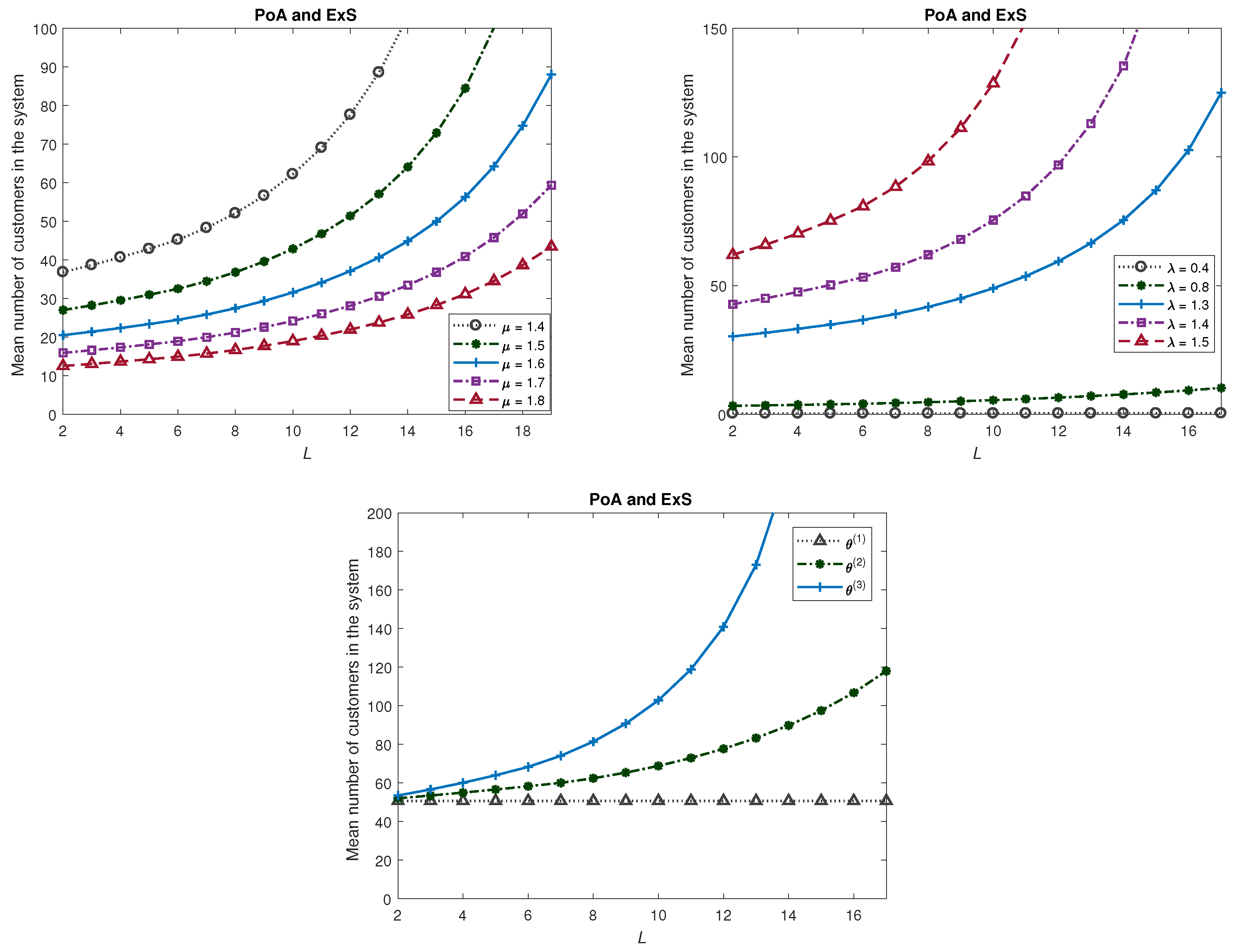
• As is to be expected, the mean number of customers in the system increases as L is increased. This is due to the fact that as L is increased, the rate of service is decreased and thus an increase in the mean number of customers in the system. However, the rate of increase (as a function of L) is higher as $\mu$ is decreased.
• $L_s$ increases as the arrival rate is increased. Furthermore, the rate of increase of $L_s$ (with respect to L) is higher as $\lambda$ is increased.
• First observe that ${\mathit{\theta }}^{\left(\mathbf{3}\right)}$ gives a higher degradation in service rates as compared to ${\mathit{\theta }}^{\left(\mathbf{1}\right)}$ and ${\mathit{\theta }}^{\left(\mathbf{2}\right)}$. We see from the third graph of Figure 1, Figure 2 and Figure 3 that more degradation in service rate gives more $L_s$ and more $P_{busy}$ but less $P_{idl\mathit{e}}$.
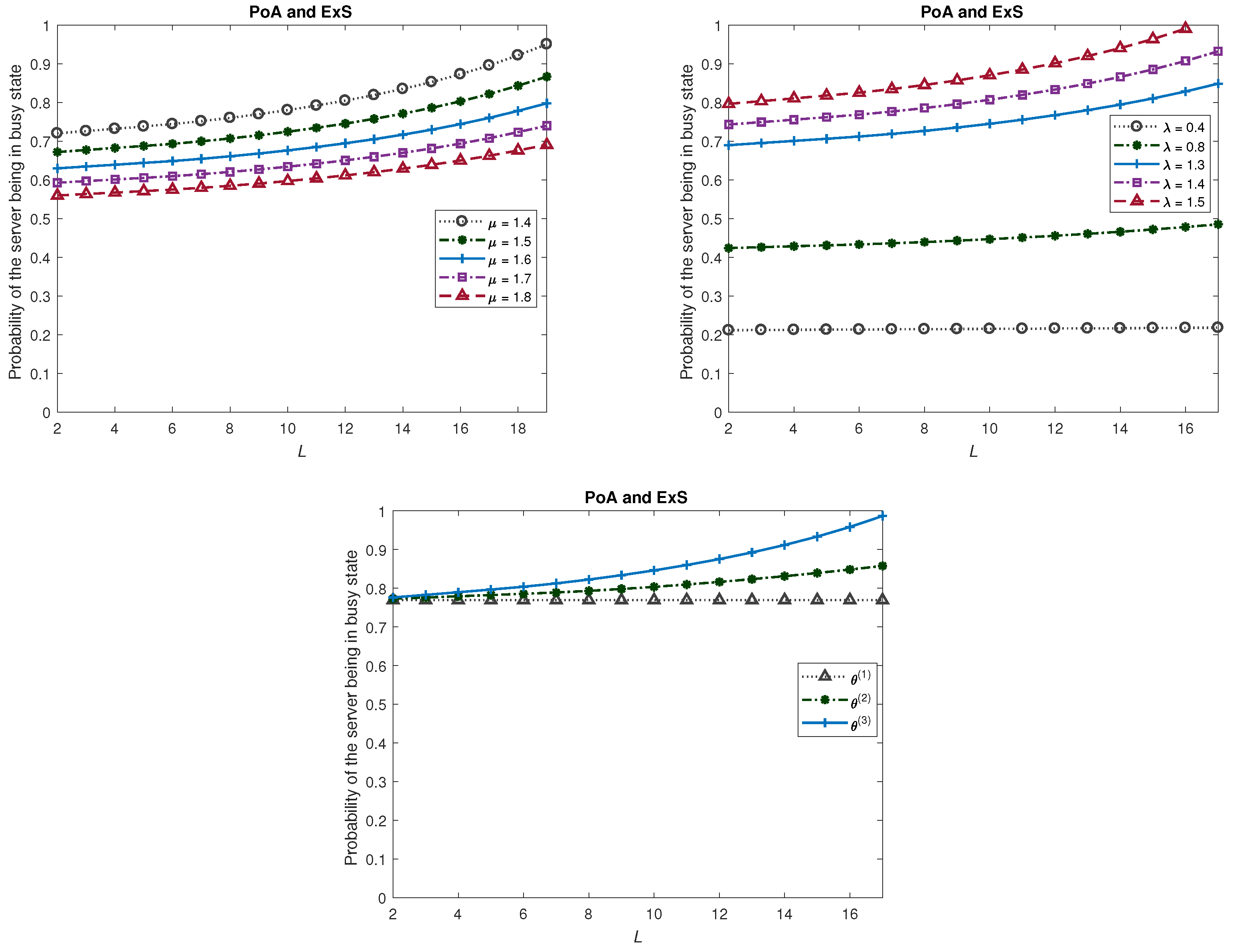
• The server will be more busy if there are more customers in the system and so is the measure $P_{busy}$. Also, an increase in L and in $\lambda$ will result in an increase in $P_{busy}$ and similarly an increase in $\mu$ will decrease the measure $P_{busy}$.
• Obviously, a higher degradation in the services provided will lead to the server being more busy and this is seen in the measure $P_{busy}$.

Example 2.

In this example, we look at Model 2 under various scenarios. Note that in this model, there is a vacation for the server. Thus, the vacation distribution is also varied. Where we need to denote the type of service and the type of vacation used, we will denote by $EE$ to indicate that both service and vacation times have Erlang (E) distribution; similarly, $EX$ will denote that the service time is Erlang and the vacation duration is exponential. Thus, the first letter represents the service process and the second one represents the vacation process.

First, we compare the degrading system with vacation with that of the classical vacation model. To compare properly, we will take the service rate for the classical vacation model to be the average of the service rates in the corresponding degrading system. That is, for the classical vacation model the service rate is taken to be $\frac{\mu }{L}{\displaystyle \sum _{i=1}^L}{\theta }_i$. In the following we fix $\lambda =1$, unless it is varied. Using the same arrival and service processes of Example 1, and looking at the vacation times to follow one of the three PH-distributions listed above, fixing $L=10,\mu =1.9,{\mu }_v=10$, and taking $\mathit{\theta }={(1,0.98,0.96,0.94,0.92,0.90,0.87,0.84,0.81,0.78)}^t$, we display the mean number of customers in the system under various scenarios in Figure 4. The figure contains the plots for both degradation system as well as for the corresponding classical queueing model with vacation. As the average service rate in the degradation system is $\left(1.9\right)\left(0.9\right)=1.71$, the classical vacation model will have the service rate fixed at 1.71.

Following are the key observations from these two figures.

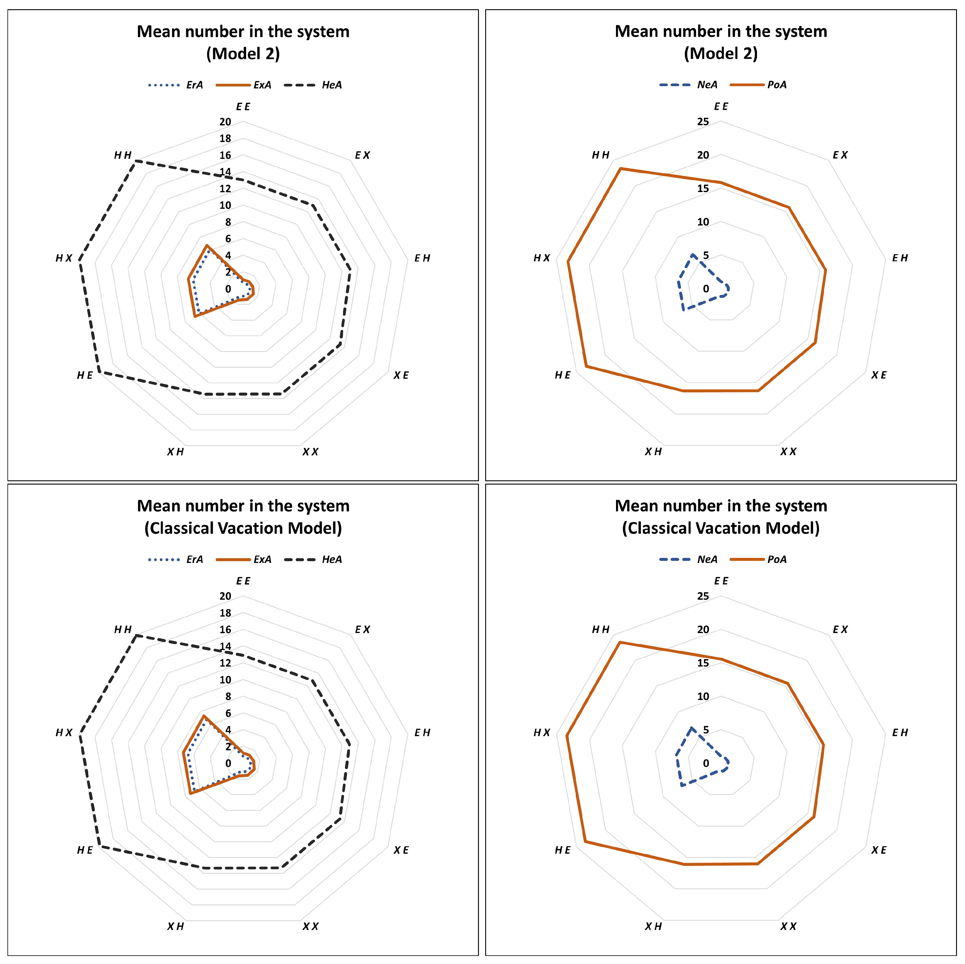
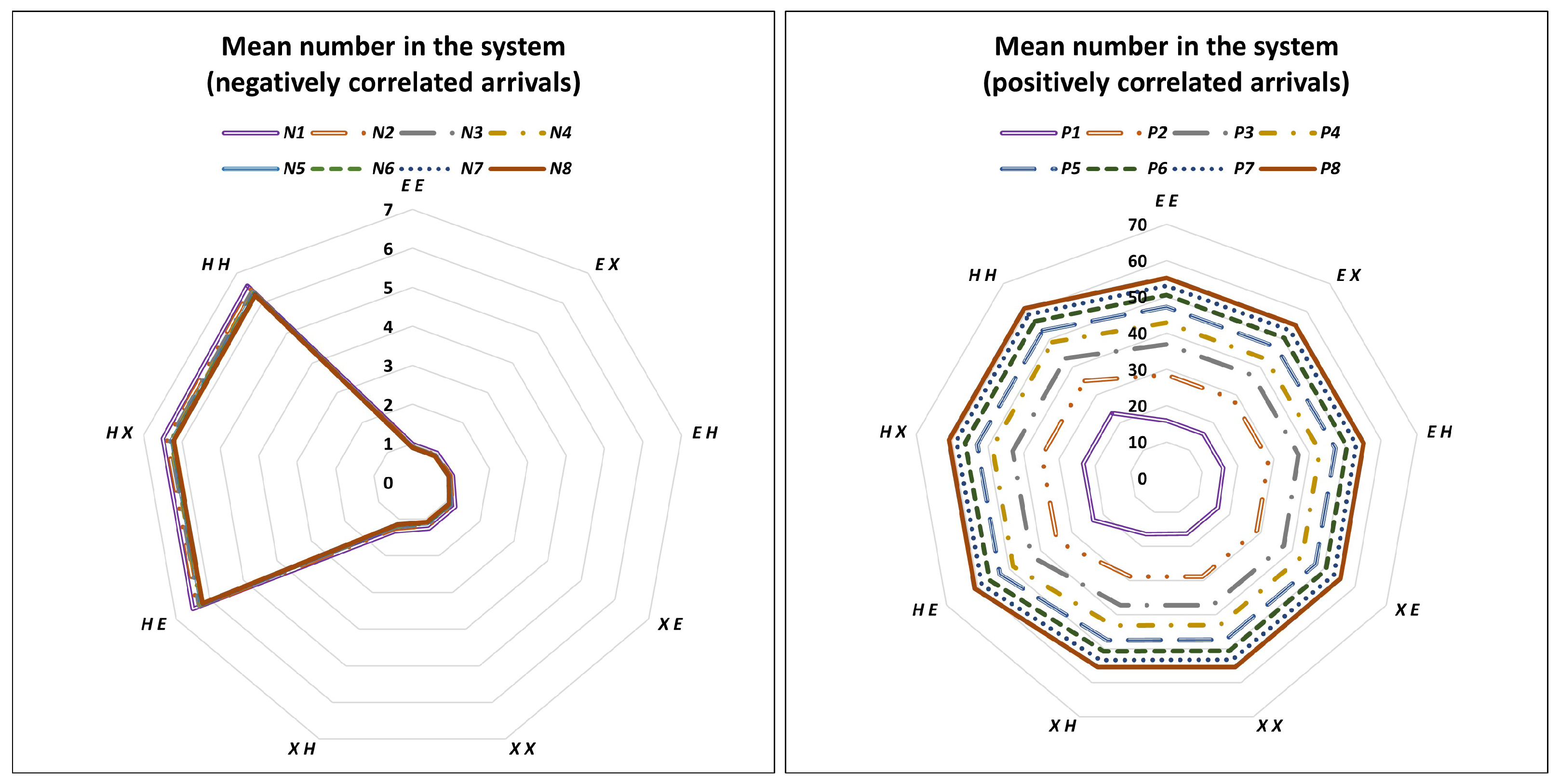
• Both the degradation and the corresponding classical vacation models have almost the same mean number of customers in the system, and also follow the same pattern as we change the service and vacation processes.
• Furthermore, the positively correlated arrival process gives the highest mean number of customers among all the considered arrival processes which reflects the role of correlation.
• The hyperexponential service gives more mean number of customers than the Erlang and exponential service.
• Erlang, exponential, and negatively correlated arrivals have the same pattern as the service and the vacation processes are varied. Similarly, the hyperexponential and positively correlated arrivals have the same pattern.

Example 3.

Next, to see the effects of positive and negative correlated arrivals, we look at more arrival processes with negative and positive correlations. Towards this end, we look at eight negatively correlated and eight positively correlated arrival processes. The correlation coefficients for the positively correlated arrivals $P1,P2,\cdots ,P8$ are 0.3267, 0.4804, 0.5786, 0.6454, 0.6935, 0.7296, 0.7577, and 0.7802, respectively. The correlation coefficients for the negatively correlated ones, $N1,N2,\cdots ,N8$, have the same values in magnitude. The standard deviations for $Ni$’s and $Pi$’s, $i=1,2,\cdots ,8$, are the same and are given by 1.0392, 1.0202, 1.0123, 1.0082, 1.0059, 1.0044, 1.0035, and 1.0028.

In Figure 5, we plot the mean number of customers in the system for the degradation system.

Following are some key observations from Figure 5.

• For the negatively correlated arrivals, as the magnitude of the correlation coefficient decreases, the mean number of costumers in the system increases.
• For the positively correlated arrivals, as the magnitude of correlation coefficient increases, the mean number in the system increases.
• Furthermore, the effect of the positively correlated arrivals is seen more than the negatively correlated arrivals as the magnitude of the correlation is varied.

Example 4.

Furthermore, the graphs of various measures for Model 2 are plotted in Figure 6, Figure 7 and Figure 8 to see the effects of the number of services done before vacation, under various scenarios. In Figure 6, Figure 7 and Figure 8, we fix $\lambda =1,\mu =1.3,{\mu }_v=5$, and $\mathit{\theta }=(1,0.98,0.96,0.94,0.92,0.90,0.87,0.84$, $0.81,0.78,0.75$, $0.72,0.69,0.66,0.63,0.60,0.57,0.54$, ${0.52,0.5)}^t$ unless these are varied. ${\mathit{\theta }}^{\left(\mathbf{1}\right)}$, ${\mathit{\theta }}^{\left(\mathbf{2}\right)}$, and ${\mathit{\theta }}^{\left(\mathbf{3}\right)}$ are same as the Example 1. For the third and the fourth graphs, namely, the ones that are displayed in the second row, seen in Figure 6, Figure 7 and Figure 8, μ is fixed to be 1.9.

Some key observations from these figures are summarized below.

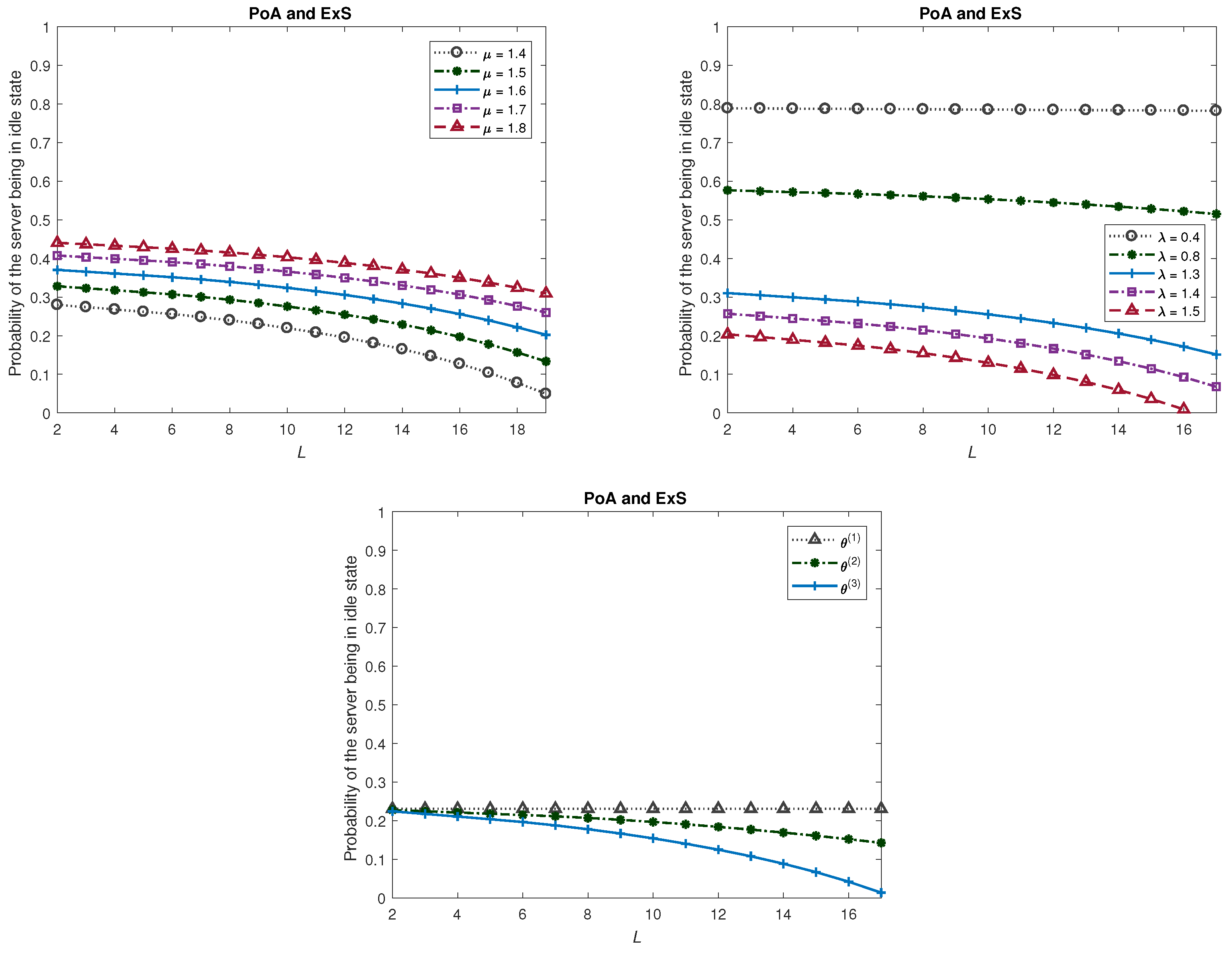
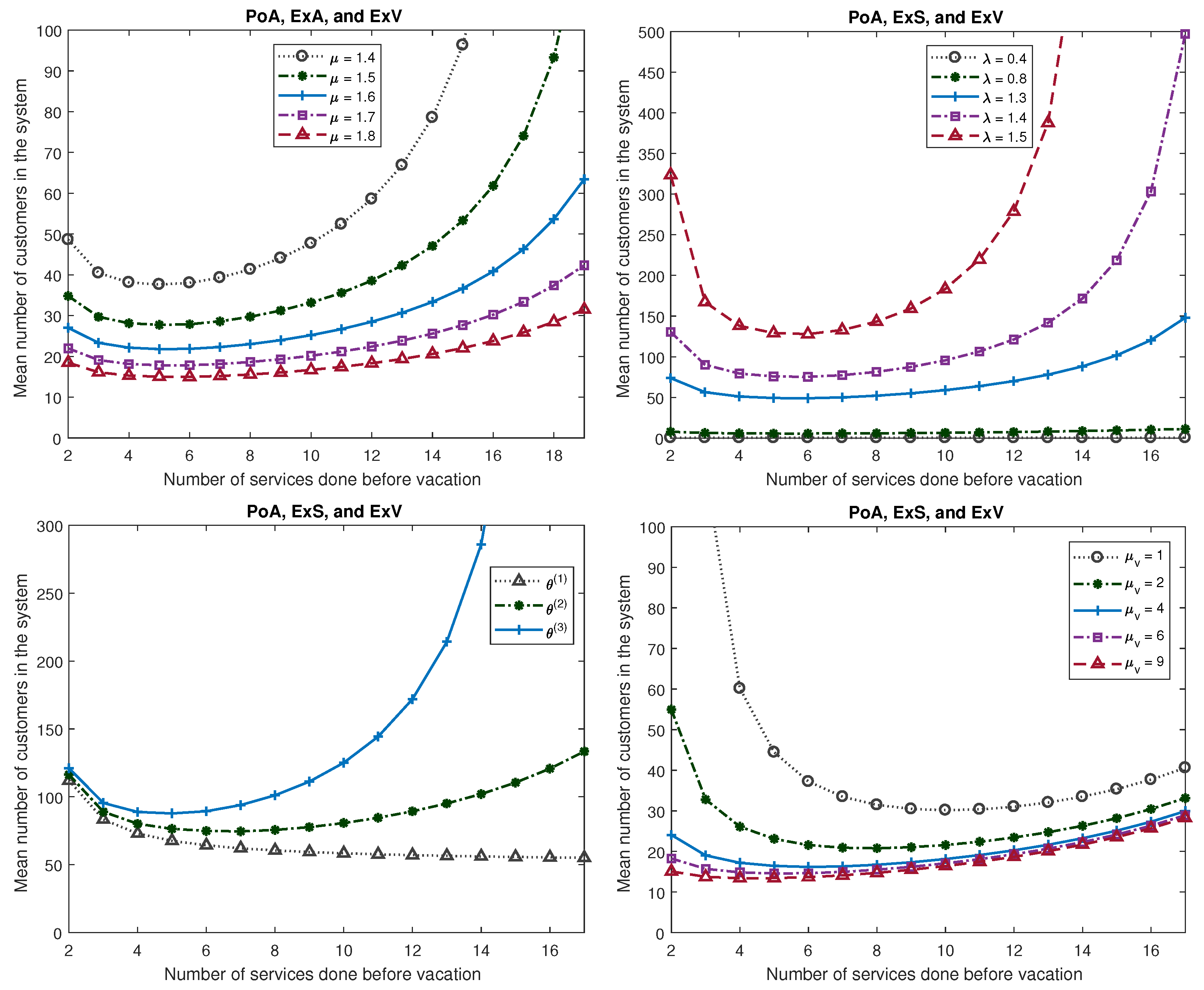
• For the mean number of customers in the system $L_s^{\left(v\right)}$:
  • $L_s^{\left(v\right)}$ decreases if there is an increase in $\mu$ as well as in ${\mu }_v$.
  • An increase in $\lambda$ results in an increase in $L_s^{\left(v\right)}$.
  • More degradation in the service rate will result in a higher value for $L_s^{\left(v\right)}$.
  • An increase in L will decrease the $L_s^{\left(v\right)}$ initially but after a certain point we notice an increase in $L_s^{\left(v\right)}$. The value of L for which the $L_s^{\left(v\right)}$ is smallest depends on all the system parameters.
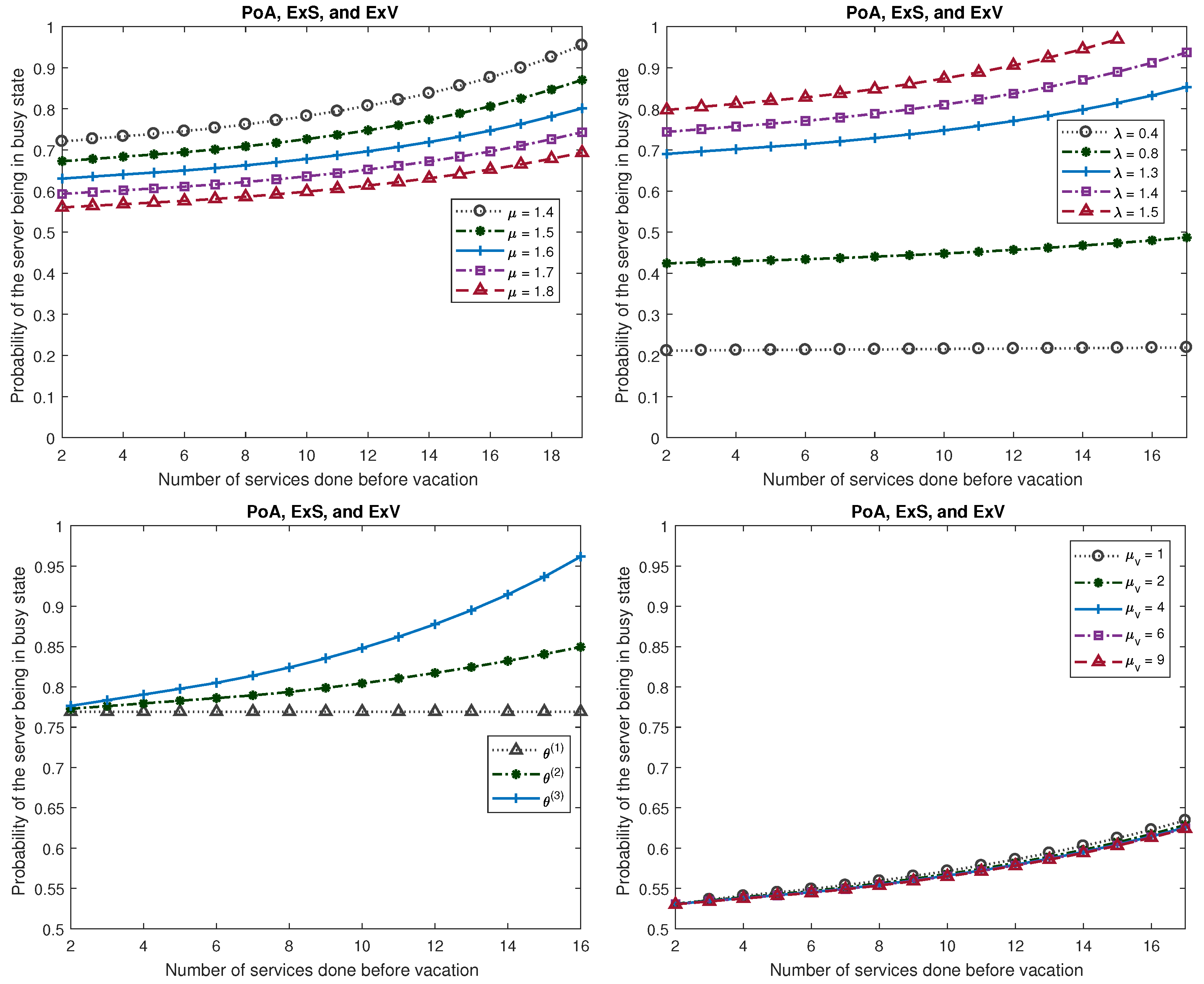
• For the probability of the server being in busy state $\left(P_{busy}\right)$:
  • An increase in $\mu$ will decrease the probability, $P_{busy}$, but an increase in $\lambda$ increases $P_{busy}$.
  • The more degradation is present in the services, the busier the server is.
  • The parameter ${\mu }_v$ has a negligible effect on $P_{busy}$ as compared to other parameters. However, an increment in ${\mu }_v$ will decrease the $P_{busy}$.
  • Increment in L will increase the $P_{busy}$.
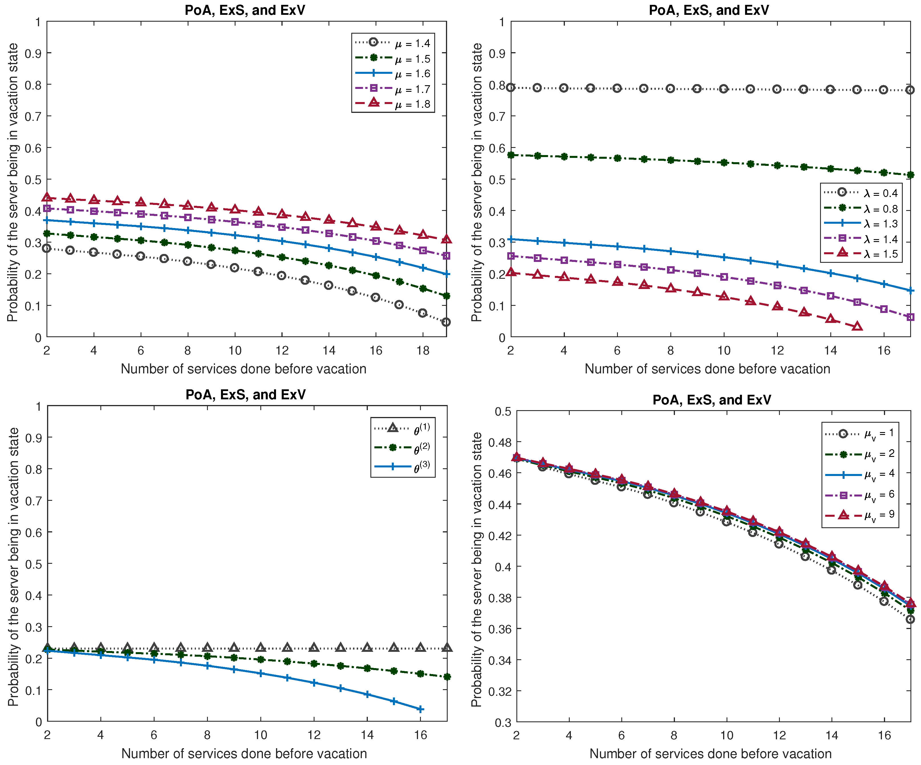
• The probability of the server being in vacation state ($P_{vacation}$) behaves opposite to the $P_{busy}$ as the system parameters are varied.

Finally, we compare Model 1 and Model 2 by looking at the figures displayed for these two models in Examples 1 and 4. In both the models, we see that all the system parameters have a similar effect on the performance measures of Model 1 as the performance measures of Model 2 have. However, Model 1 has less mean number of customers in the system as compared to Model 2. This is due to the fact that the degraded services are instantaneously fixed in Model 1, whereas in Model 2 it takes a random time to fix the same. We displayed graphs only for the positively correlated arrivals and the exponential distribution for both service and vacation processes as we observed all the processes of arrival, service, and vacation have a similar effect as the system parameters are varied.

Example 5.

In this example, we compare Model 1 to the classical MAP/PH/1 model. For this we consider negatively and positively correlated arrivals with the same $D_0$ and $D_1$ provided in Example 1. For the service process, we consider Erlang distribution and hyperexponential distribution same as in Example 1. For Model 1, we consider $\mu =1.4$, $L=10$, and $\theta =(1,0.98,0.96,0.94,$${0.92,0.90,0.87,0.84,0.81,0.78)}^t$. For the classical $MAP/PH/1$ model, service rate is taken to be the average of the service rates of Model 1, which is $1.26$.

In

Table 1. Performance measures for classical $MAP/PH/1$ model, Model 1, and Model 2.

Model	Processes	${\mathit{L}}_{\mathit{s}}$	${\mathit{P}}_{\mathit{busy}}$	${\mathit{P}}_{\mathit{idle}}/{\mathit{P}}_{\mathit{vacation}}$
Classical $MAP/PH/1$ model	NeA, ErS	2.22305	0.790528	0.206349
	NeA, HyS	58.92956	0.82926	0.206349
	PoA, ErS	24.16811	0.791647	0.206349
	PoA, HyS	82.19010	0.848347	0.206349
Model 1	NeA, ErS	2.07631	0.762403	0.237597
	NeA, HyS	60.92105	0.779311	0.220689
	PoA, ErS	23.63030	0.773938	0.226062
	PoA, HyS	84.05024	0.782954	0.217046
Model 2	NeA, ErS	2.45311	0.768110	0.231890
	NeA, HyS	71.03092	0.781503	0.218497
	PoA, ErS	26.56992	0.777106	0.222894
	PoA, HyS	96.61144	0.784809	0.215191

, we display some key measures for the classical MAP/PH/1 and the two models studied here. We observe that Model 1 has higher values for $L_s$ and $P_{busy}$ than the corresponding classical $MAP/PH/1$ model which is obvious and shows the impact of the degrading services. We see that for the processes NeA and ErS, Model 1 has less $L_s$ and less $P_{busy}$ than the classical $MAP/PH/1$ model. This is because the server becomes frequently idle in Model 1 and the service rate is instantaneously restored to the original rate, which results in having a lower $L_s$. To compare it with Model 2, we consider the exponential distribution of vacation process with mean rate ${\mu }_v=5$. Model 2 has the highest mean number of customers in the system due to being on vacation for a random time.

5. Conclusions

In this paper, we studied the degradation that commonly occurs in many industries, notably in service sectors, in the context of $MAP/PH/1$-type queues. We studied two types of models. In Model 1, the degrading service rate is reset to its initial rate instantaneously after a fixed number of services or when the server becomes idle. In Model 2, it requires some random time to fix the service rate to resume to its normal rate. Stability conditions for both the models are derived and some important performance measures are also given. Numerical examples are provided and the comparison of both the models is also done. This study can be extended to include breakdowns and repairs of the server, and for multiple server systems. These are currently being investigated.

References

1. Ejaz, I.; Alvarado, M.; Gautam, N.; Gebraeel, N.; Lawley, M. Condition-based maintenance for queues with degrading servers. IEEE Trans. Autom. Sci. Eng. 2019, 16, 1750–1762. [Google Scholar] [CrossRef]
2. Doshi, B.T. Queueing systems with vacations—A survey. Queueing Syst. 1986, 1, 29–66. [Google Scholar] [CrossRef]
3. Tian, N.; Zhang, Z.G. Vacation Queueing Models: Theory and Applications; Springer Publishers: New York, NY, USA, 2006. [Google Scholar]
4. Servi, L.; Finn, S. M/M/1 queue with working vacations (M/M/1/WV). Perform. Eval. 2002, 50, 41–52. [Google Scholar] [CrossRef]
5. Kim, J.; Choi, D.; Chae, K. Analysis of queue-length distribution of the M/G/1 queue with working vacations. In Proceedings of the Hawaii International Conference on Statistics and Related Fields, Honolulu, HI, USA, 5–8 June 2003. [Google Scholar]
6. Baba, Y. Analysis of a GI/M/1 queue with multiple working vacations. Oper. Res. Lett. 2005, 33, 201–209. [Google Scholar] [CrossRef]
7. Li, J.; Tian, N. The M/M/1 queue with working vacations and vacation interruptions. J. Syst. Sci. Syst. Eng. 2007, 16, 121–127. [Google Scholar] [CrossRef]
8. Chakravarthy, S.R. A multi-server synchronous vacation model with thresholds and a probabilistic decision rule. Eur. J. Oper. Res. 2007, 182, 305–320. [Google Scholar] [CrossRef]
9. Chakravarthy, S.R. Analysis of a multi-server queue with Markovian arrivals and synchronous phase type vacations. Asia-Pac. J. Oper. Res. 2009, 26, 85–113. [Google Scholar] [CrossRef]
10. Tian, N.; Li, J.; Zhang, Z.G. Matrix-analytic method and working vacation queues—A survey. Int. J. Inf. Manag. Sci. 2009, 20, 603–633. [Google Scholar]
11. Zhang, M.; Hou, Z. Performance analysis of MAP/G/1 queue with working vacations and vacation interruption. Appl. Math. Model. 2011, 35, 1551–1560. [Google Scholar] [CrossRef] [Green Version]
12. Chakravarthy, S.R. Analysis of a multi-server queueing model with vacations and optional secondary services. Math. Appl. 2013, 41, 127–151. [Google Scholar] [CrossRef]
13. Chakravarthy, S.R. Analysis of MAP/PH1, PH2/1 queue with vacations and optional secondary services. Appl. Math. Model. 2013, 37, 8886–8902. [Google Scholar] [CrossRef]
14. Sreenivasan, C.; Chakravarthy, S.R.; Krishnamoorthy, A. MAP/PH/1 queue with working vacations, vacation interruptions and N policy. Appl. Math. Model. 2013, 37, 3879–3893. [Google Scholar] [CrossRef]
15. Alfa, A. Some decomposition results for a class of vacation queues. Oper. Res. Lett. 2014, 42, 140–144. [Google Scholar] [CrossRef]
16. Yang, D.-Y.; Wu, C.-H. Cost-minimization analysis of a working vacation queue with N-policy and server breakdowns. Comput. Ind. Eng. 2015, 82, 151–158. [Google Scholar] [CrossRef]
17. Chakravarthy, S.R.; Shruti; Kulshrestha, R. A queueing model with server breakdowns, repairs, vacations, and backup server. Oper. Res. Perspect. 2020, 7, 100131. [Google Scholar] [CrossRef]
18. Jain, M.; Dhibar, S.; Sanga, S.S. Markovian working vacation queue with imperfect service, balking and retrial. J. Ambient. Intell. Humaniz. Comput. 2021, 1–17. [Google Scholar] [CrossRef]
19. Chakravarthy, S.R. A Comparative Study of Vacation Models Under Various Vacation Policies: A Simulation Approach. In Mathematical Modeling and Computation of Real-Time Problems; CRC Press: Boca Raton, FL, USA, 2021; pp. 3–20. [Google Scholar]
20. Marcus, M.; Minc, H. Survey of Matrix Theory and Matrix Inequalities; Allyn and Bacon: Boston, MA, USA, 1964. [Google Scholar]
21. Steeb, W.H.; Hardy, Y. Matrix Calculus and Kronecker Product: A Practical Approach to Linear and Multilinear Algebra; World Scientific Publishing: Singapore, 2011. [Google Scholar]
22. Neuts, M.F. A versatile Markovian point process. J. Appl. Probab. 1979, 16, 764–779. [Google Scholar] [CrossRef]
23. Neuts, M.F. Probability distributions of phase type. Liber Amicorum Prof. Emeritus H. Florin, Dept. Math. Univ. Louvain, Belgium 1975, 173–206. [Google Scholar]
24. Lucantoni, D.M.; Meier-Hellstern, K.S.; Neuts, M.F. A single server queue with server vacations and a class of non-renewal arrival processes. Adv. Appl. Probab. 1990, 22, 676–705. [Google Scholar] [CrossRef]
25. Chakravarthy, S.R. The batch Markovian arrival process: A review and future work. In Advances in Probability Theory and Stochastic Processes; Krishnamoorthy, A., Raju, N., Ramaswami, V., Eds.; Notable Publications Inc.: Princeton, NJ, USA, 2001; pp. 21–39. [Google Scholar]
26. Artalejo, J.R.; Gomez-Corral, A. Markovian arrivals in stochastic modelling: A survey and some new results (invited article with discussion: Rafael Perez-Ocaon, Miklos Telek and Yiqiang Q. Zhao). SORT Stat. Oper. Res. Trans. 2010, 34, 101–156. [Google Scholar]
27. Chakravarthy, S.R. Markovian Arrival Process. Wiley Encyclopedia of Operations Research and Management Science. 2010. Available online: https://onlinelibrary.wiley.com/doi/abs/10.1002/9780470400531.eorms0499 (accessed on 15 June 2010).
28. Basharin, G.; Naumov, V.; Samouylov, K. On Markovian modelling of arrival processes. Stat. Pap. 2018, 59, 1533–1540. [Google Scholar] [CrossRef]
29. He, Q.M. Fundamentals of Matrix-Analytic Methods; Springer: New York, NY, USA, 2014. [Google Scholar]
30. Dudin, A.N.; Klimenok, V.I.; Vishnevsky, V.M. The Theory of queueing Systems with Correlated Flows; Springer: Cham, Switzerland, 2020. [Google Scholar] [CrossRef]
31. Neuts, M.F. Matrix-Geometric Solutions in Stochastic Models: An Algorithmic Approach; Johns Hopkins University: Baltimore, MD, USA, 1981. [Google Scholar]
Figure 1. Mean number of customers in the system (Model 1).
Mathematics 09 02387 g001
Figure 2. Probability of the server being in busy state (Model 1).
Mathematics 09 02387 g002
Figure 3. Probability of the server being in idle state (Model 1).
Mathematics 09 02387 g003
Figure 4. Mean number of customers in the system for Model 2 under various scenarios.
Mathematics 09 02387 g004
Figure 5. Mean number of customer in the system for negatively correlated and positively correlated arrivals (Model 2).
Mathematics 09 02387 g005
Figure 6. Mean number of customer in the system (Model 2).
Mathematics 09 02387 g006
Figure 7. Probability of the server being in busy state (Model 2).
Mathematics 09 02387 g007
Figure 8. Probability of the server being in vacation state (Model 2).
Mathematics 09 02387 g008