Planar Typical Bézier Curves with a Single Curvature Extremum

Abstract

This paper focuses on planar typical Bézier curves with a single curvature extremum, which is a supplement of typical curves with monotonic curvature by Y. Mineur et al. We have proven that the typical curve has at most one curvature extremum and given a fast calculation formula of the parameter at the curvature extremum. This will allow designers to execute a subdivision at the curvature extremum to obtain two pieces of typical curves with monotonic curvature. In addition, we put forward a sufficient condition for typical curve solutions under arbitrary degrees for the G1 interpolation problem. Some numerical experiments are provided to demonstrate the effectiveness and efficiency of our approach.

1. Introduction

In CAGD (Computer Aided Geometric Design) applications, it is preferable to generate aesthetically pleasing surfaces, which are usually modeled by a set of feature curves with the required fairing shape. The shape of such curves and surfaces is usually influenced by curvature distribution; therefore, curvature plays a critical role in measuring the fairness of curves and surfaces. Farin [1,2] pointed out that a curve is fair on the condition that it has relatively few monotonic curvature variation segments. There is much research that discusses how to control curvature distribution based on Bézier or B-spline curves [1,3,4,5], which are effective design tools in CAD (Computer Aided Design) systems. However, the conditions of conventional methods are complex, which leads to a limitation in usefulness.

Some research concentrates on realizing the monotonic variation of curvature. Different from traditional methods, a new class of geometric methods have been developed. Mineur et al. [6] defined a special 2D Bézier curve with monotonic curvature called a “typical curve”, which has particular geometric constraints on control edges. In 2006, Farin [7] put forward the concept of “Class A Bézier curves”, a generalization of typical curves in 3D space. The key to obtain monotonic curvature and torsion is to construct a Class A matrix. However, the conditions of a Class A matrix cannot guarantee monotonic curvature [8], and several counter-examples have verified this [9]. Recently, new sufficient conditions of a 2D and 3D Class A matrix have been proposed [10,11]. In addition, Wang et al. gave other sufficient conditions for monotonic curvature of planar Bézier curves and B-spline curves without a transformation matrix [12,13].

Although the conditions of monotonic curvature have been widely studied, it is inevitable that curvature extrema are sometimes produced, such as with an interpolation problem. In recent years, articles have focused on how to control the local maxima of curvature at given points. According to [14], points with a curvature extremum are a salient geometric feature of a curve, because human beings are more sensitive to minima and maxima of curvature. To better control curvature distribution, it makes sense to identify the local maxima of curvature. Ref. [15] introduced kappa curves to interpolate a series of points with local curvature maxima only appearing at given points. Kappa curves consist of piecewise-quadratic Bézier curves and have G2 continuity over the whole curve except for the inflection points, where only G1 continuity remains. In [16], the authors similarly used piecewise rational curves as interpolatory curves to reproduce circles. Other extensions of kappa curves include two types of ϵκ-curves [17], which make it possible to control the magnitudes of local maximum curvature. In [18], a class of C2 interpolating splines were introduced, showing the superiority of C2 continuity as well as local support compared to kappa curves.

However, for the interpolatory methods mentioned above, obtaining the parameter at the curvature extremum requires much computation. Considering the generality of objective curves for the interpolation problem, we relaxed the constraints of typical Bézier curves and provided a fast calculation of the parameter at the curvature extremum under arbitrary degrees.

This paper is organized as follows. Section 2 introduces typical Bézier curves with only one curvature extremum. Section 3 gives the formula of the parameter at the curvature extremum. Section 4 shows the application in G1 interpolation. Finally, conclusions are given in Section 5.

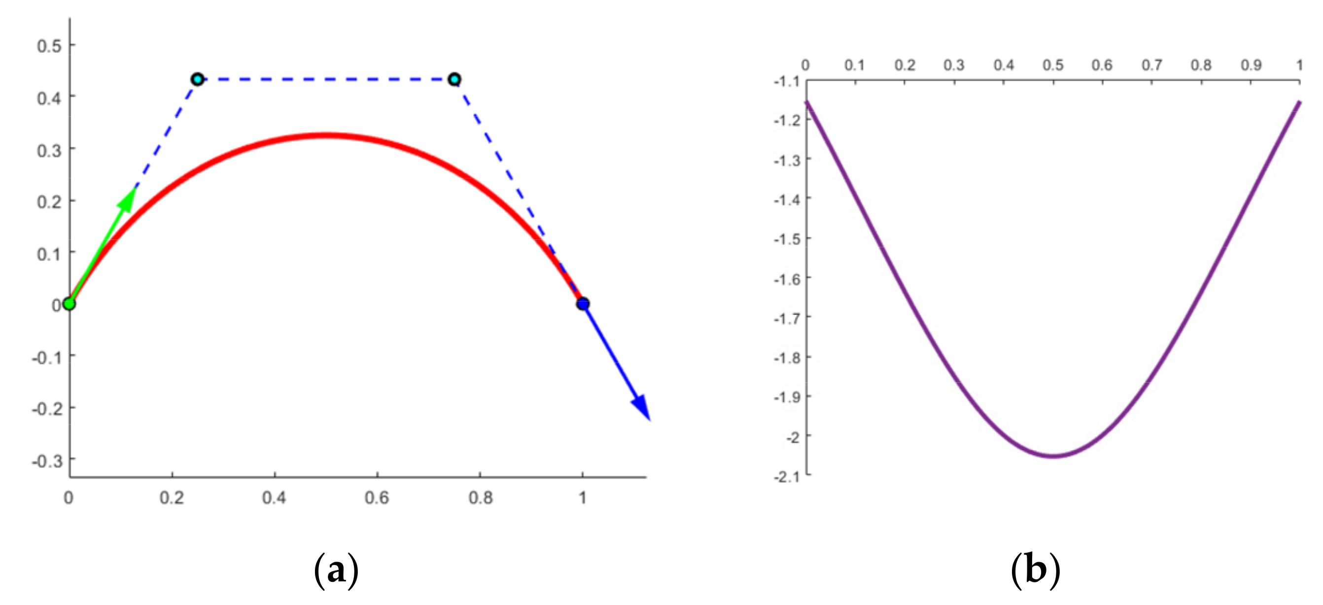
2. Typical Bézier Curves with One Curvature Extremum

A planar k-degree Bézier curve in parametric form is defined by

$$\mathit{P}(t)={\displaystyle \sum _{i=0}^k{\mathit{b}}_i{B}_{i,k}}(t),t\in \left[0,1\right]$$

(1)

where $\left\{{\mathit{b}}_i\right\}$, $\left\{B_{i,k}(t)=C_k^i{t}^i{\left(1-t\right)}^{k-i}\right\}$ are control points and Bernstein polynomials, respectively. In this paper we agree that all vectors are column vectors in a two-dimensional plane.

Typical Bézier curves belong to a special subset of Bézier curves, whose control edge vector $\Delta {\mathit{b}}_i={\mathit{b}}_{i+1}-{\mathit{b}}_i$ is given as follows:

$$\Delta {\mathit{b}}_i={\mathit{M}}^i\cdot \Delta {\mathit{b}}_0,i=0,1,\dots ,k-1$$

(2)

where $\mathit{M}=s\cdot \left(\begin{array}{cc}\cos \theta & -\sin \theta \\ \sin \theta & \cos \theta \end{array}\right)$ with $s>0$ and $\theta \in [-\pi ,\pi ]$, $\Delta {\mathit{b}}_0\ne 0$ is the first control edge vector. In this way, we get $〈\Delta {\mathit{b}}_{i-1},\Delta {\mathit{b}}_i〉\equiv \theta$ and $‖\Delta {\mathit{b}}_i‖/‖\Delta {\mathit{b}}_{i-1}‖\equiv s$, where 〈 〉 denotes the angle formed by two vectors and ‖ ‖ denotes the Euclidean norm of a given vector. If $s\cdot \cos \theta \ge 1$ ($s\ge 1$) or $s\le \cos \theta$ ($0<s<1$), then typical curves have monotonic curvature variation [6]. In this paper, we mainly focus on the complementary relation

$$\left\{\begin{array}{l}s\cdot \cos \theta <1,s\ge 1\hfill \\ s>\cos \theta ,0<s<1\hfill \end{array}\right.,$$

(3)

and prove that there exists only one curvature extremum under this condition.

Theorem 1.

Planar typical Bézier curves with Equation (3) have only one curvature extremum.

Proof. 

In essence, the parameter direction for $0<s<1$ is opposite to that of $s\ge 1$, so the conclusion for $0<s<1$ can be made in the same way as for $s\ge 1$. Similarly, the curve with rotation angle for $\theta \in [-\pi ,0)$ is symmetric to that for $\theta \in [0,\pi ]$. Hence, only the condition for $s\ge 1$ and $\theta \in [0,\pi ]$ will be verified.

The derivative of a Bernstein polynomial can be written as a combination of two lower degree polynomials:

$$\frac{\mathrm{d}{B}_{i,k}(t)}{\mathrm{d}t}=k\left(B_{i-1,k-1}(t)-B_{i,k-1}(t)\right).$$

Therefore, based on Equation (1), the first and second derivatives of the Bézier curve can be expressed as [2]

$${\mathit{P}}^{\prime }(t)=k{\displaystyle \sum _{i=0}^{k-1}{\mathit{b}}_i^1{B}_{i,k-1}}(t),$$

(4)

$${\mathit{P}}^{″}(t)=k\left(k-1\right){\displaystyle \sum _{i=0}^{k-2}{\mathit{b}}_i^2{B}_{i,k-2}}(t),$$

(5)

where ${\mathit{b}}_i^1={\mathit{b}}_{i+1}-{\mathit{b}}_i=\Delta {\mathit{b}}_i$ and ${\mathit{b}}_i^2={\mathit{b}}_{i+1}^1-{\mathit{b}}_i^1$ are the control points of first and second derivatives, respectively. Recall that the relative curvature is given by

$$\kappa (t)=\frac{\det \left({\mathit{P}}^{\prime }(t),{\mathit{P}}^{″}(t)\right)}{{‖{\mathit{P}}^{\prime }(t)‖}^3},$$

(6)

where $\det \left({\mathit{P}}^{\prime }(t),{\mathit{P}}^{″}(t)\right)$ is the determinant of matrix $\left({\mathit{P}}^{\prime }(t),{\mathit{P}}^{″}(t)\right)$. Since $\det \left({\mathit{P}}^{\prime }(t),{\mathit{P}}^{″}(t)\right)=‖{\mathit{P}}^{\prime }(t)‖\cdot ‖{\mathit{P}}^{″}(t)‖\cdot \sin 〈{\mathit{P}}^{\prime }(t),{\mathit{P}}^{″}(t)〉$, Equation (6) can be transformed to

$$\kappa (t)=\frac{‖{\mathit{P}}^{″}(t)‖}{‖{\mathit{P}}^{\prime }(t)‖}\cdot \frac{\sin 〈{\mathit{P}}^{\prime }(t),{\mathit{P}}^{″}(t)〉}{‖{\mathit{P}}^{\prime }(t)‖}.$$

(7)

Based on Equations (4) and (5), $\mathit{P}(t)$, ${\mathit{P}}^{\prime }(t)$ and ${\mathit{P}}^{″}(t)$ can be represented as in Figure 1. Since the translation operation has no effect on the geometric property of $\mathit{P}(t)$ and its derivatives ${\mathit{P}}^{\prime }(t)$, ${\mathit{P}}^{″}(t)$, the i-th control point ${\mathit{b}}_i$ is taken as the origin and then ${\mathit{b}}_i^{}{\mathit{b}}_{i+1}^{}={\mathit{b}}_i^{}{\mathit{b}}_i^1$ as in Figure 1b.

Following Figure 1 and Equation (2), it can be inferred that

$$\frac{‖{\mathit{b}}_i{\mathit{b}}_{i+1}^1‖}{‖{\mathit{b}}_i{\mathit{b}}_i^1‖}=\frac{‖{\mathit{b}}_i{\mathit{b}}_{i+2}^1‖}{‖{\mathit{b}}_i{\mathit{b}}_{i+1}^1‖},\angle {\mathit{b}}_{i+1}^1{\mathit{b}}_i^{}{\mathit{b}}_i^1=\angle {\mathit{b}}_{i+2}^1{\mathit{b}}_i^{}{\mathit{b}}_{i+1}^1,$$

which indicates $△{\mathit{b}}_i^{}{\mathit{b}}_i^1{\mathit{b}}_{i+1}^1\sim △{\mathit{b}}_i^{}{\mathit{b}}_{i+1}^1{\mathit{b}}_{i+2}^1$. Similarly, we find that $△{\mathit{b}}_i^{}{\mathit{b}}_i^1{\mathit{b}}_{i+1}^1$, $△{\mathit{b}}_i^{}{\mathit{b}}_{i+1}^1{\mathit{b}}_{i+2}^1$, $△{\mathit{b}}_i^{}{\mathit{b}}_i^2{\mathit{b}}_{i+1}^2$, $△{\mathit{b}}_i^{}{\mathit{b}}_{i,k-3}^1{\mathit{b}}_{i+1,k-3}^1$, $△{\mathit{b}}_i^{}{\mathit{b}}_{i,k-2}^1{\mathit{b}}_{i+1,k-2}^1$ and $△{\mathit{b}}_i^{}{\mathit{b}}_{i,k-3}^2{\mathit{b}}_{i+1,k-3}^2$ are six similar triangles. Since $s\cdot \cos \theta <1$ ($s\ge 1$, $\theta \in [0,\pi ]$), ${\mathit{b}}_{i+1}^1$ will be located in the green region in Figure 2, then $\angle {\mathit{b}}_i^{}{\mathit{b}}_i^1{\mathit{b}}_{i+1}^1$ is an acute angle and the corresponding triangle $△{\mathit{b}}_i^{}{\mathit{b}}_i^1{\mathit{b}}_{i+1}^1$ is an acute triangle. Hence, the above triangles are six similar acute triangles.

Suppose ${\mathit{b}}_h^{}$ is the endpoint of the segment ${\mathit{b}}_i^{}{\mathit{b}}_h^{}$, which is perpendicular to the segment ${\mathit{b}}_{i,k-3}^1{\mathit{b}}_{i+1,k-3}^1$ (Figure 3), and the corresponding parameter at ${\mathit{b}}_h^{}$ is $t^{\ast }$. Since $△{\mathit{b}}_i^{}{\mathit{b}}_{i,k-3}^1{\mathit{b}}_{i+1,k-3}^1$ is an acute triangle due to the similarity, the endpoint ${\mathit{b}}_h^{}$ is located in the segment ${\mathit{b}}_{i,k-3}^1{\mathit{b}}_{i+1,k-3}^1$. Accordingly, $\angle {\mathit{b}}_i^{}{\mathit{b}}_{i,k-2}^1{\mathit{b}}_{i+1,k-3}^1$ first increases from $\angle {\mathit{b}}_i^{}{\mathit{b}}_{i,k-3}^1{\mathit{b}}_{i+1,k-3}^1$ ($<\pi /2$) to $\pi /2$ then decreases to $\angle {\mathit{b}}_i^{}{\mathit{b}}_{i+1,k-3}^1{\mathit{b}}_{i,k-3}^1$. Meanwhile $‖{\mathit{b}}_i^{}{\mathit{b}}_{i,k-2}^1‖$ first decreases from $‖{\mathit{b}}_i^{}{\mathit{b}}_{i,k-3}^1‖$ to the minimum $‖{\mathit{b}}_i^{}{\mathit{b}}_h^{}‖$ then increases to $‖{\mathit{b}}_i^{}{\mathit{b}}_{i+1,k-3}^1‖$. It is not hard to draw the conclusions (I), (II) and (III), as follows.

(I).

$\sin 〈{\mathit{P}}^{\prime }(t),{\mathit{P}}^{″}(t)〉$ increases in $\left[0,t^{\ast }\right]$ then decreases in $\left[t^{\ast },1\right]$.

By $△{\mathit{b}}_i^{}{\mathit{b}}_{i,k-3}^2{\mathit{b}}_{i+1,k-3}^2\sim △{\mathit{b}}_i^{}{\mathit{b}}_{i,k-2}^1{\mathit{b}}_{i+1,k-2}^1$, ${\mathit{b}}_{i,k-3}^2{\mathit{b}}_i\parallel {\mathit{b}}_{i+1,k-3}^1{\mathit{b}}_{i,k-3}^1$ and the de Casteljau algorithm, we get

$$〈{\mathit{P}}^{\prime }(t),{\mathit{P}}^{″}(t)〉=\angle {\mathit{b}}_{i,k-3}^2{\mathit{b}}_i{\mathit{b}}_{i,k-2}^1=\angle {\mathit{b}}_i{\mathit{b}}_{i,k-2}^1{\mathit{b}}_{i,k-3}^1.$$

$\angle {\mathit{b}}_i{\mathit{b}}_{i,k-2}^1{\mathit{b}}_{i,k-3}^1$ first increases from acute angle $\angle {\mathit{b}}_i{\mathit{b}}_{i,k-3}^1{\mathit{b}}_{i+1,k-3}^1$ to $\pi /2$, where $t=t^{\ast }$ and then decreases to $\angle {\mathit{b}}_i{\mathit{b}}_{i+1,k-3}^1{\mathit{b}}_{i,k-3}^1$, so does $〈{\mathit{P}}^{\prime }(t),{\mathit{P}}^{″}(t)〉$. Consequently, $〈{\mathit{P}}^{\prime }(t),{\mathit{P}}^{″}(t)〉$ and $\sin 〈{\mathit{P}}^{\prime }(t),{\mathit{P}}^{″}(t)〉$ is increasing for $\left[0,t^{\ast }\right]$ and decreasing for $\left[t^{\ast },1\right]$.

(II).

$\frac{‖{\mathit{P}}^{″}(t)‖}{‖{\mathit{P}}^{\prime }(t)‖}$ increases in $\left[0,t^{\ast }\right]$ then decreases in $\left[t^{\ast },1\right]$.

From $△{\mathit{b}}_i^{}{\mathit{b}}_{i,k-3}^2{\mathit{b}}_{i+1,k-3}^2\sim △{\mathit{b}}_i^{}{\mathit{b}}_{i,k-2}^1{\mathit{b}}_{i+1,k-2}^1$ and the de Casteljau algorithm, we can obtain

$$\frac{‖{\mathit{P}}^{″}(t)‖}{‖{\mathit{P}}^{\prime }(t)‖}=\frac{‖{\mathit{b}}_i{\mathit{b}}_{i,k-3}^2‖}{‖{\mathit{b}}_i{\mathit{b}}_{i,k-2}^1‖}.$$

In the above equation, $‖{\mathit{b}}_i{\mathit{b}}_{i,k-2}^1‖$ decreases in $\left[0,t^{\ast }\right]$ and then increases in $\left[t^{\ast },1\right]$ while $‖{\mathit{b}}_i{\mathit{b}}_{i,k-3}^2‖$ keeps constant. For this reason, we deduce $\frac{‖{\mathit{P}}^{″}(t)‖}{‖{\mathit{P}}^{\prime }(t)‖}$ increases in $\left[0,t^{\ast }\right]$ and then decreases in $\left[t^{\ast },1\right]$.

(III).

$\frac{1}{‖{\mathit{P}}^{\prime }(t)‖}$ increases in $\left[0,t^{\ast }\right]$ and then decreases in $\left[t^{\ast },1\right]$.

By $△{\mathit{b}}_i^{}{\mathit{b}}_{i,k-3}^1{\mathit{b}}_{i+1,k-3}^1\sim △{\mathit{b}}_i^{}{\mathit{b}}_{i,k-2}^1{\mathit{b}}_{i+1,k-2}^1$, there holds $\frac{‖{\mathit{b}}_i{\mathit{b}}_{i,k-2}^1‖}{‖{\mathit{P}}^{\prime }(t)‖}=\frac{‖{\mathit{b}}_i{\mathit{b}}_{i,k-3}^1‖}{‖{\mathit{b}}_i{\mathit{b}}_{i,k-2}^1‖}$, thus we get

$$\frac{1}{‖{\mathit{P}}^{\prime }(t)‖}=\frac{‖{\mathit{b}}_i{\mathit{b}}_{i,k-3}^1‖}{{‖{\mathit{b}}_i{\mathit{b}}_{i,k-2}^1‖}^2}.$$

In acute triangle $△{\mathit{b}}_i^{}{\mathit{b}}_{i,k-3}^1{\mathit{b}}_{i+1,k-3}^1$, $‖{\mathit{b}}_i{\mathit{b}}_{i,k-2}^1‖$ is decreasing for $\left[0,t^{\ast }\right]$ then increasing for $\left[t^{\ast },1\right]$ while $‖{\mathit{b}}_i{\mathit{b}}_{i,k-3}^1‖$ remains invariant; therefore $\frac{1}{‖{\mathit{P}}^{\prime }(t)‖}$ first increases and then decreases.

Based on (I), (II) and (III), the curvature function of Equation (7) first increases and then decreases, which indicates that $\kappa (t)$ possesses a single curvature extremum for $t\in \left[0,1\right]$ when $s\cdot \cos \theta <1$ ($s\ge 1$). □

Figure 4 and Figure 5 illustrate two typical Bézier curves with a unimodal curvature profile for $s\ge 1$ and $0<s<1$, respectively.

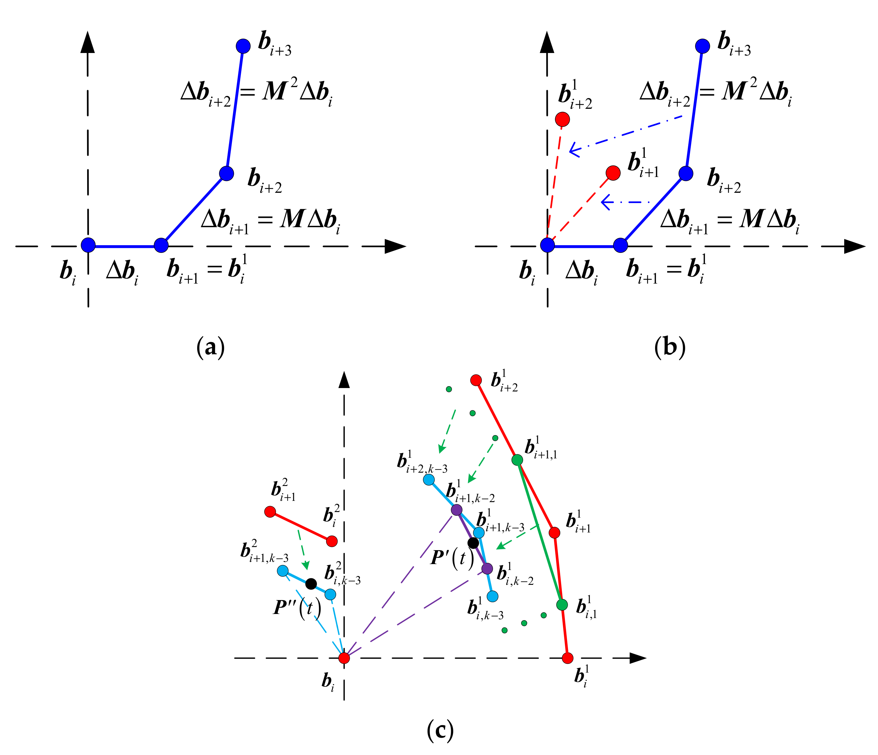
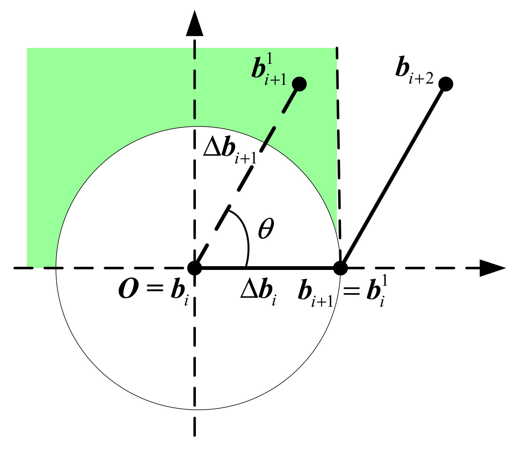
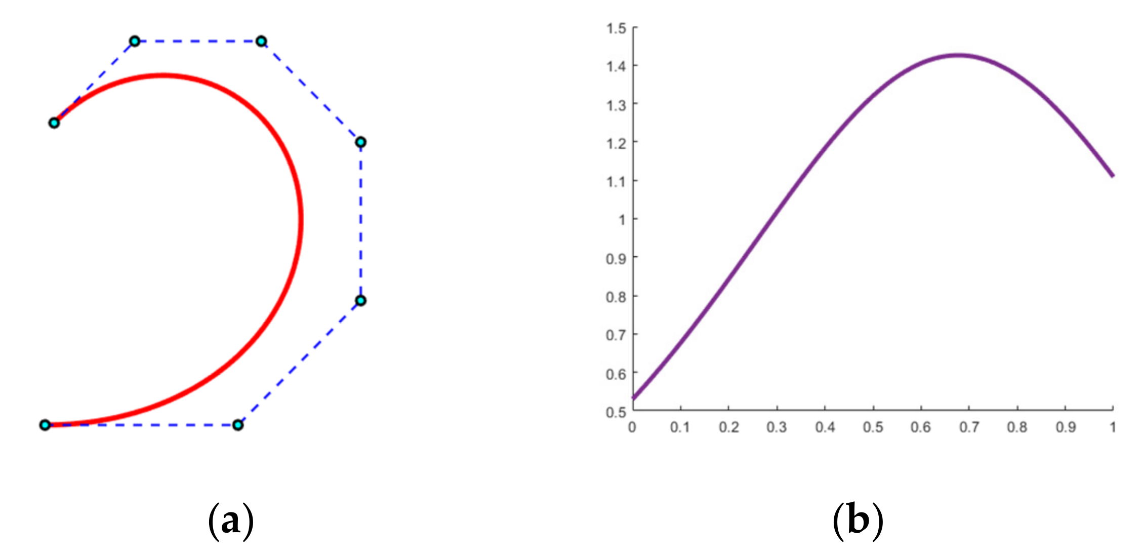
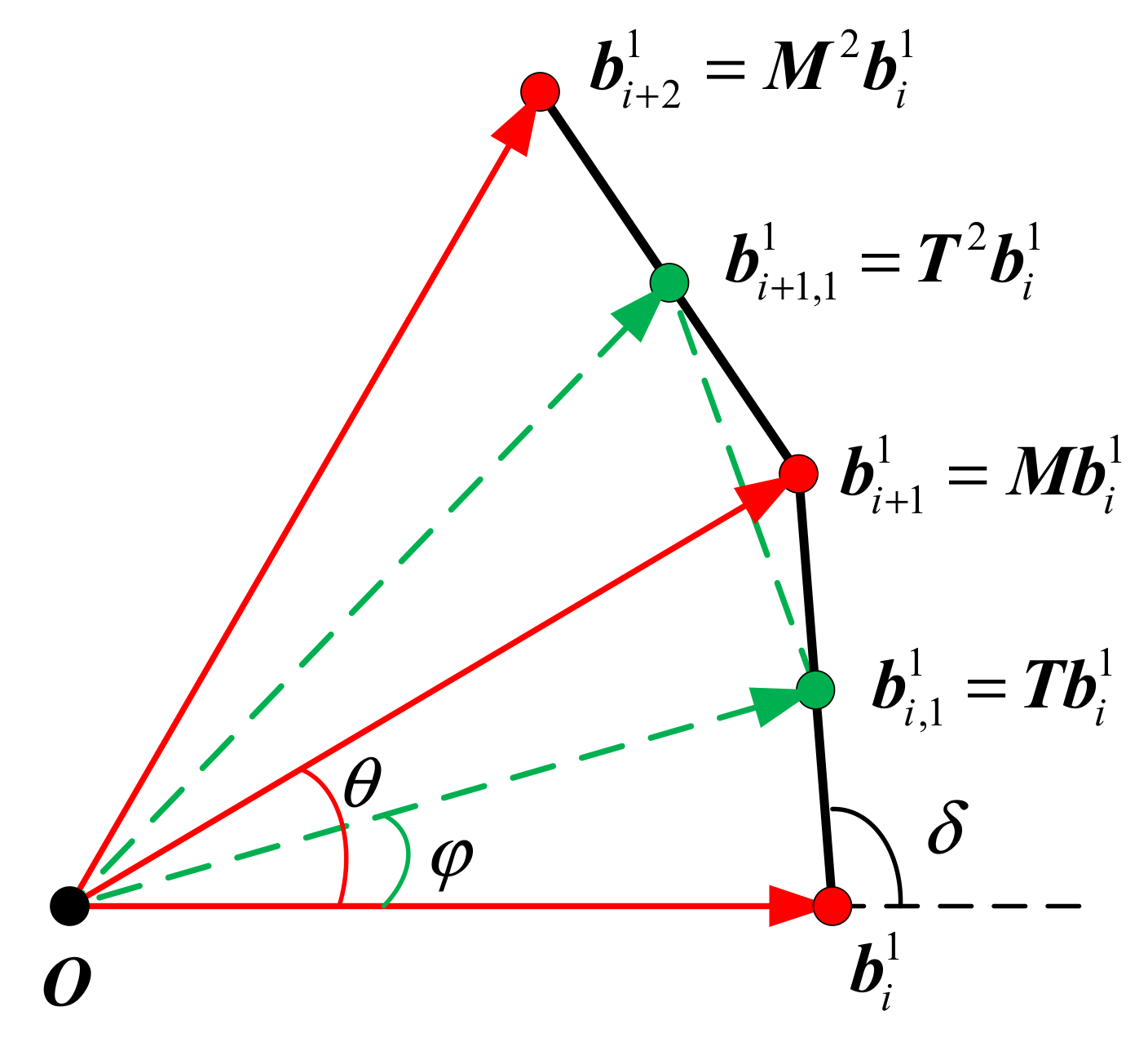
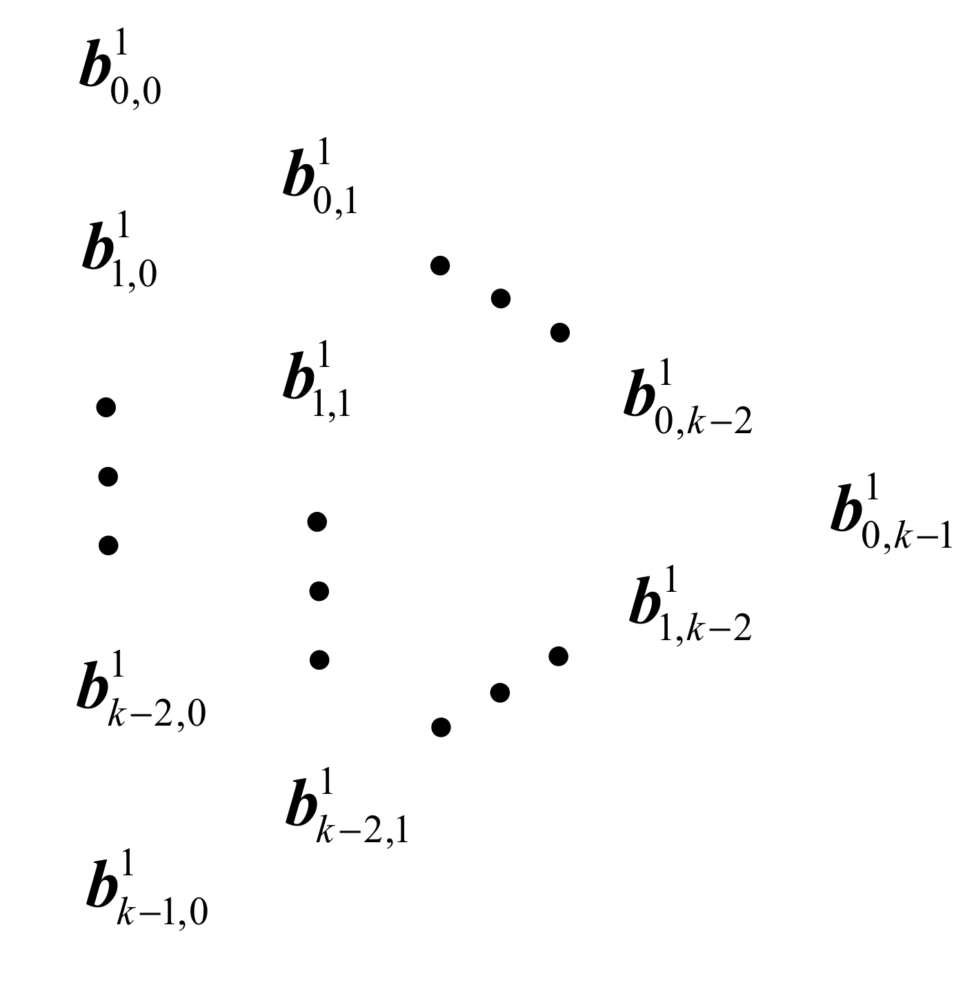
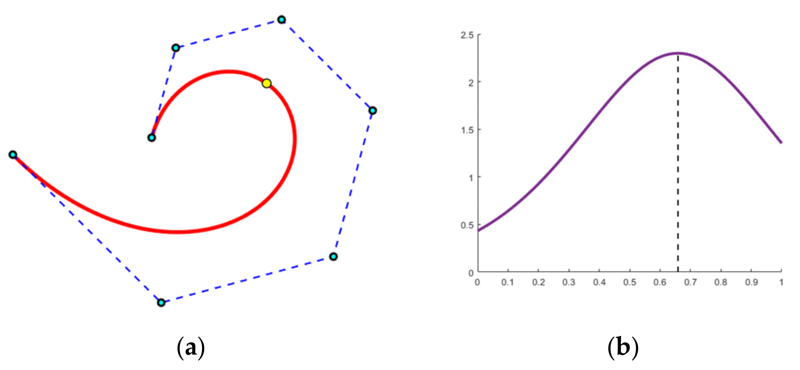
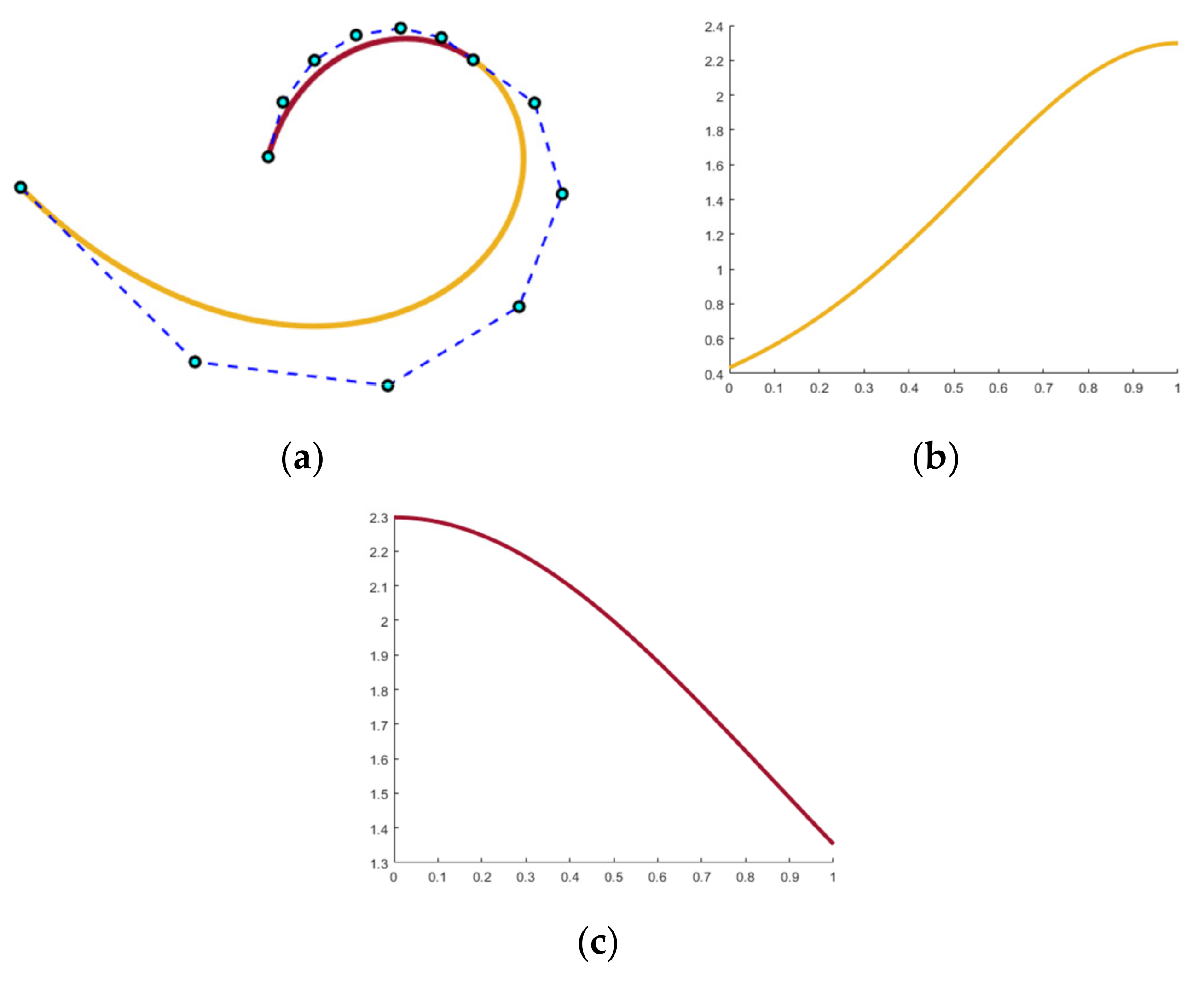
3. Parameter Formula and Subdivision at Curvature Extremum

In this section, we provide a fast formula to calculate parameter $t^{\ast }$ at the point with curvature extremum, which also proves Theorem 1 in an algebraic way. Then we show the subdivision at $t^{\ast }$ and prove that the two obtained segments belong to typical curves with monotonic curvature.

3.1. Fast Parameter Formula

Let ${\mathit{b}}_{i,1}^1=\left(1-t\right){\mathit{b}}_i^1+t{\mathit{b}}_{i+1}^1=\left(1-t\right){\mathit{b}}_i^1+t\mathit{M}{\mathit{b}}_i^1$ be the i-th auxiliary point in the first recursive level by the de Casteljau algorithm. Here we introduce a new transformation $\mathit{T}\left(t\right)=\left(1-t\right)\mathit{I}+t\mathit{M}$ to describe linear interpolation between adjacent control edges of a typical Bézier curve (Figure 6), where $\mathit{I}$ is second order identity matrix. Take $h=\frac{‖{\mathit{b}}_{i,1}^1‖}{‖{\mathit{b}}_i^1‖}$ and $\phi =〈{\mathit{b}}_i^1,{\mathit{b}}_{i,1}^1〉$ as the scale factor and rotation angle of $\mathit{T}\left(t\right)$ for ${\mathit{b}}_{i,1}^1=\mathit{T}{\mathit{b}}_i^1$ (Figure 6). They can be specifically expressed as (see Appendix A)

$$h=\sqrt{{\left(1-t\right)}^2+2t\left(1-t\right)s\cdot \cos \theta +{\left(ts\right)}^2},$$

(8)

$$\sin \phi =\frac{st\cdot \sin \theta }{h}.$$

(9)

From the de Casteljau algorithm (Figure 7), the i-th auxiliary point of recursive level m of the first derivative satisfies

$${\mathit{b}}_{i,m}^1=\left(1-t\right){\mathit{b}}_{i,m-1}^1+t{\mathit{b}}_{i+1,m-1}^1=\mathit{T}\left(t\right){\mathit{b}}_{i,m-1}^1$$

(10)

where $m=0,1,\dots ,k-1$, $i=0,1,\dots ,k-1-m$ and ${\mathit{b}}_{i,0}^1={\mathit{b}}_i^1$. We can rewrite the first derivative of the typical Bézier curve as

$${\mathit{P}}^{\prime }(t)=k{\displaystyle \sum _{i=0}^{k-1}{\mathit{b}}_i^1{B}_{i,k-1}}(t)=k\cdot {\mathit{b}}_{0,k-1}^1=k\cdot {\mathit{T}}^{k-1}\left(t\right){\mathit{b}}_{0,0}^1=k\cdot {\mathit{T}}^{k-1}\left(t\right){\mathit{b}}_0^1.$$

(11)

Similarly, the second derivative of the typical Bézier curve can be rewritten as

$${\mathit{P}}^{″}(t)=k\left(k-1\right)\cdot {\mathit{T}}^{k-2}\left(t\right){\mathit{b}}_0^2.$$

(12)

Therefore, the curvature $\kappa (t)$ in Equation (7) now is

$$\kappa (t)=\frac{‖k\left(k-1\right)\cdot {\mathit{T}}^{k-2}\left(t\right){\mathit{b}}_0^2‖}{‖k\cdot {\mathit{T}}^{k-1}\left(t\right){\mathit{b}}_0^1‖}\cdot \frac{\sin 〈k\cdot {\mathit{T}}^{k-1}\left(t\right){\mathit{b}}_0^1,k\left(k-1\right)\cdot {\mathit{T}}^{k-2}\left(t\right){\mathit{b}}_0^2〉}{‖k\cdot {\mathit{T}}^{k-1}\left(t\right){\mathit{b}}_0^1‖}.$$

(13)

After simplification, we get

$$\kappa (t)=\frac{k-1}{k}\cdot \frac{1}{h^k}\frac{‖{\mathit{b}}_0^2‖}{‖{\mathit{b}}_0^1‖}\cdot \frac{\sin \left(\delta -\phi \right)}{‖{\mathit{b}}_0^1‖}.$$

(14)

By the sine theorem, there holds $\frac{\sin \left(\delta -\phi \right)}{‖\mathit{O}{\mathit{b}}_i^1‖}=\frac{\sin \delta }{‖\mathit{O}{\mathit{b}}_{i,1}^1‖}$ in $△\mathit{O}{\mathit{b}}_i^1{\mathit{b}}_{i,1}^1$ and $\frac{\sin \delta }{‖\mathit{O}{\mathit{b}}_{i+1}^1‖}=\frac{\sin \theta }{‖{\mathit{b}}_i^1{\mathit{b}}_{i+1}^1‖}$ in $△\mathit{O}{\mathit{b}}_i^1{\mathit{b}}_{i+1}^1$, respectively (Figure 6); thus, we can obtain

$$\sin \left(\delta -\phi \right)=\frac{s\sin \theta }{h}\frac{‖{\mathit{b}}_i^1‖}{‖{\mathit{b}}_i^2‖}(i=0,1,\dots ,k-2).$$

The curvature function of Equation (14) is then converted to

$$\kappa (t)=\frac{k-1}{k}\cdot \frac{1}{h^k}\frac{‖{\mathit{b}}_0^2‖}{{‖{\mathit{b}}_0^1‖}^2}\cdot \frac{\sin \delta }{h}=\frac{k-1}{k}\cdot \frac{s\sin \theta }{‖{\mathit{b}}_0^1‖}\cdot \frac{1}{h^{k+1}}$$

(15)

Taking the derivative in Equation (15), we can obtain ${\kappa }^{\prime }(t)=-\frac{\left(k-1\right)\left(k+1\right)}{k}\cdot \frac{s\sin \theta }{‖{\mathit{b}}_0^1‖}\cdot \frac{h^{\prime }}{h^{k+2}}$. From Equation (8), $h^{\prime }=\frac{t-1+s\sin \theta \left(1-2t\right)+s^{2}t}{h}$; thus the derivative of the curvature is

$${\kappa }^{\prime }(t)=-\frac{\left(k-1\right)\left(k+1\right)}{k}\cdot \frac{s\sin \theta }{‖{\mathit{b}}_0^1‖}\cdot \frac{\left(s^2-2s\cos \theta +1\right)t+s\cos \theta -1}{h^{k+3}}$$

(16)

The sign of ${\kappa }^{\prime }(t)$ is related to $\left(s^2-2s\cos \theta +1\right)t+s\cos \theta -1$, which is a linear function of $t$ and changes sign at most once in $t\in \left[0,1\right]$, so the number of curvature extremum is either 0 or 1. Let ${\kappa }^{\prime }(t^{\ast })=0$ and we get

$$t^{\ast }=\frac{1-s\cos \theta }{s^2-2s\cos \theta +1}$$

(17)

Since $s^2-2s\cos \theta +1={\left(s-\cos \theta \right)}^2+{\sin }^2\theta \ge 0$, the equal sign holds only when $\theta =0$ and $s=1$. Under this condition, the typical Bézier curve degenerates into a straight line, and the curvature equals zero constantly. For the non-degeneration case, we aim to find out the relation between $s$ and $\theta$ such that $t^{\ast }\in \left(0,1\right)$, which means that ${\kappa }^{\prime }(t)$ changes sign exactly once for $t\in \left[0,1\right]$ and the corresponding typical Bézier curve will have a single curvature extremum. Thus, only when $\cos \theta <s<1/\cos \theta$ there is $0<t^{\ast }<1$, i.e., $s\cos \theta <1$ for $s\ge 1$ and $s>\cos \theta$ for $0<s<1$. Otherwise, there is $t^{\ast }\notin \left(0,1\right)$ and the typical Bézier curve will have monotonic curvature for $t\in \left[0,1\right]$.

For $t^{\ast }\notin \left(0,1\right)$, whether curvature increases or decreases depends on the sign of ${\kappa }^{\prime }(t)$, which is concerned with $\sin \theta$ and $\left(s^2-2s\cos \theta +1\right)t+s\cos \theta -1$. We draw the domain for curvature variation in $s-\theta$ coordinate system and divide it into several regions (Figure 8). The horizontal axis is limited between $-\pi$ and $\pi$, while the vertical axis extends infinitely upward from 0. The colored areas and curves in Figure 8 are symmetric with respect to $\theta =0$.

Equation (17) also gives a fast method to calculate the parameter at the curvature extremum. In particular, when $s=1$, $t^{\ast }\equiv 0.5$ for all $\theta \ne 0$. In this case, the typical Bézier curve and associated curvature plot are symmetric with respect to parameter $t=0.5$ (see Figure 9).

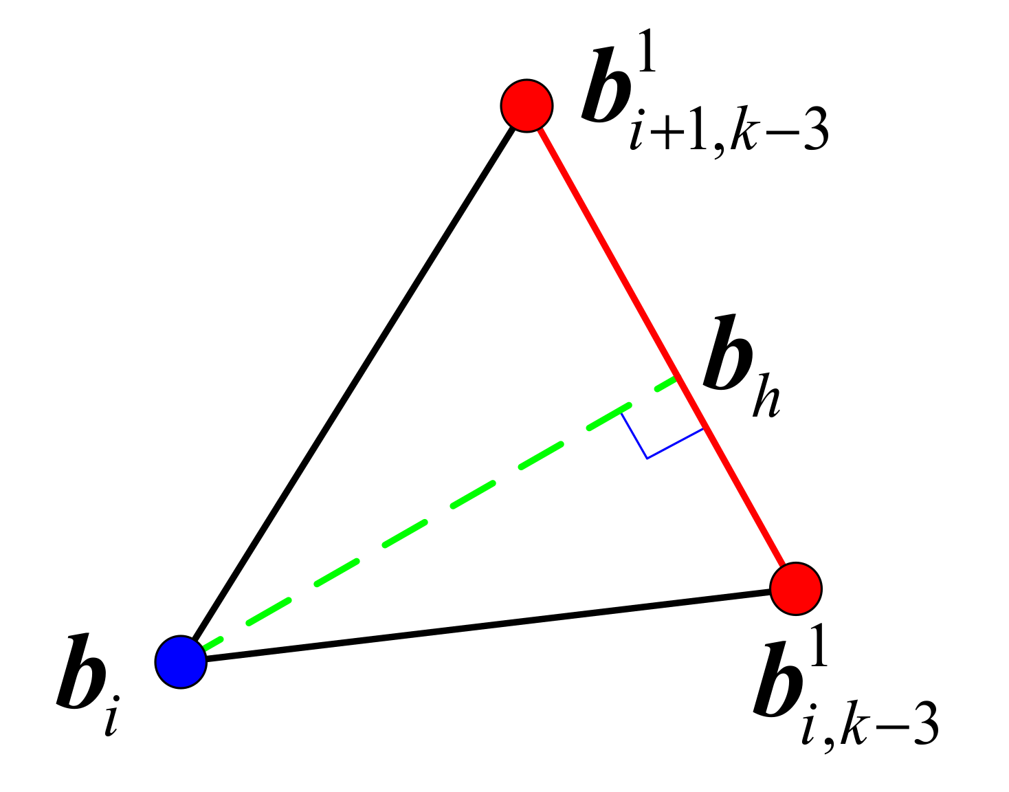
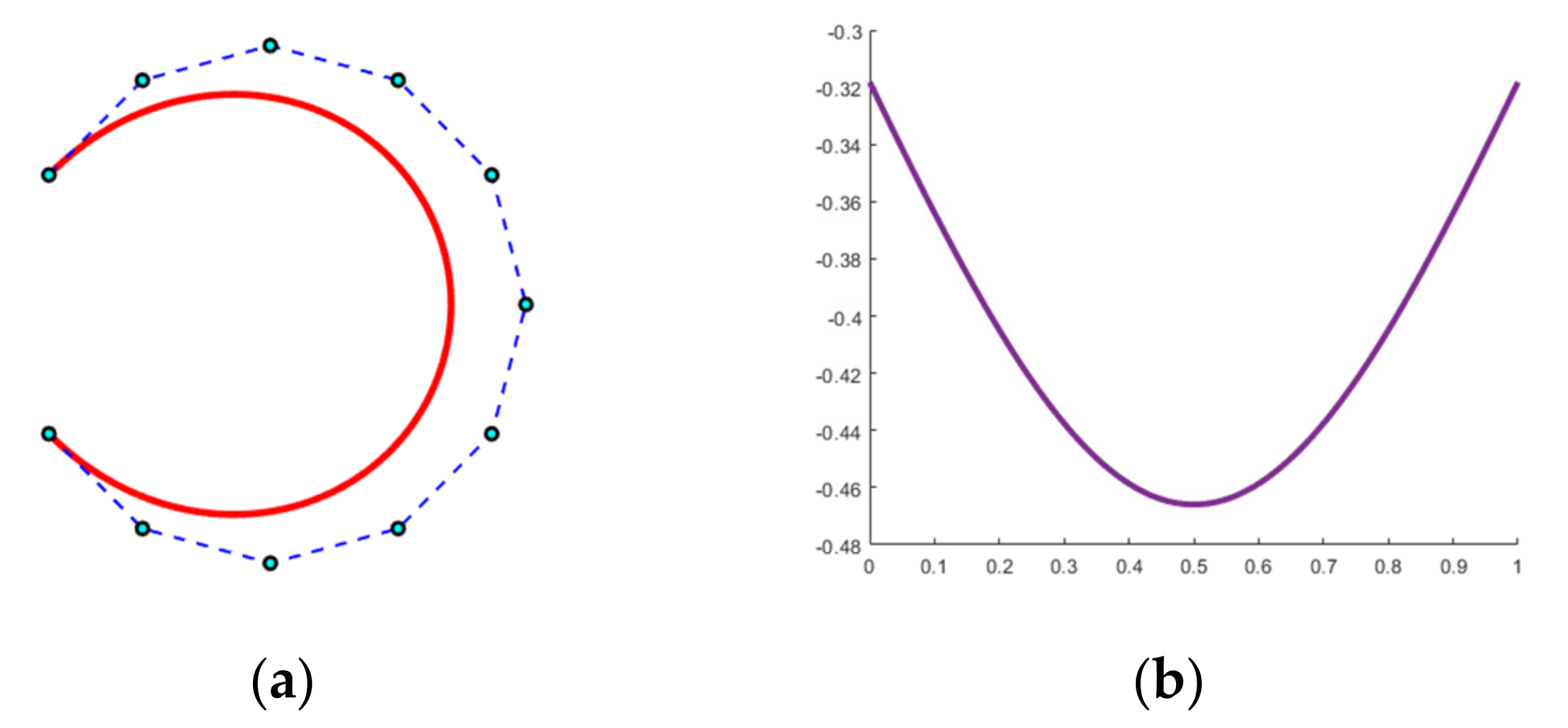
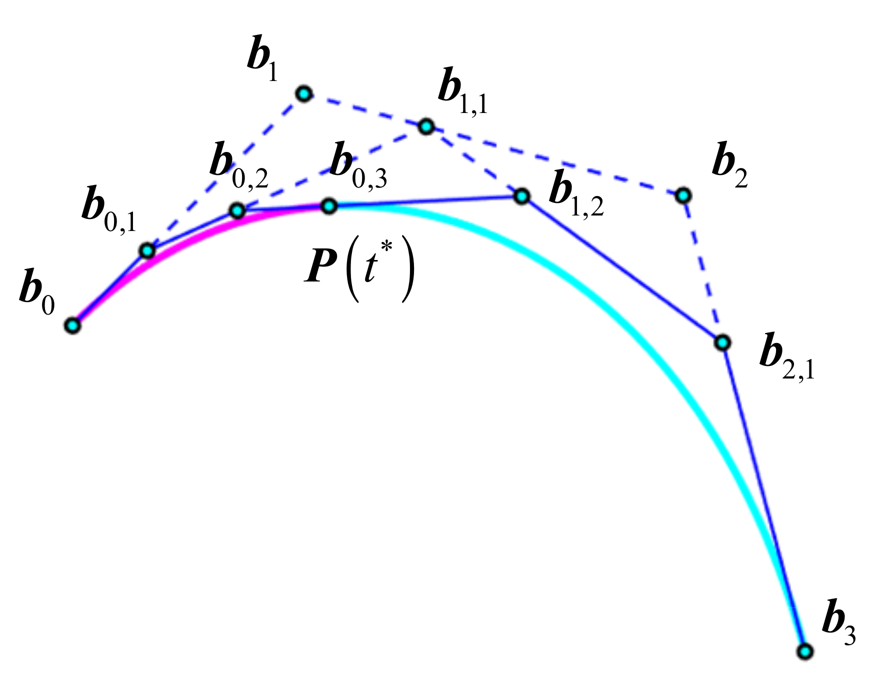
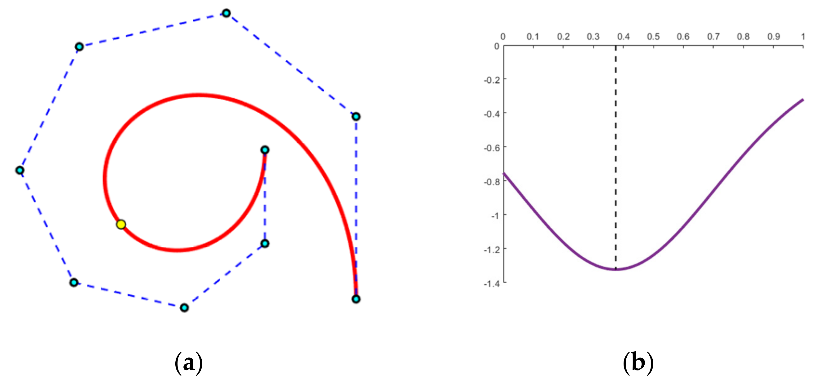
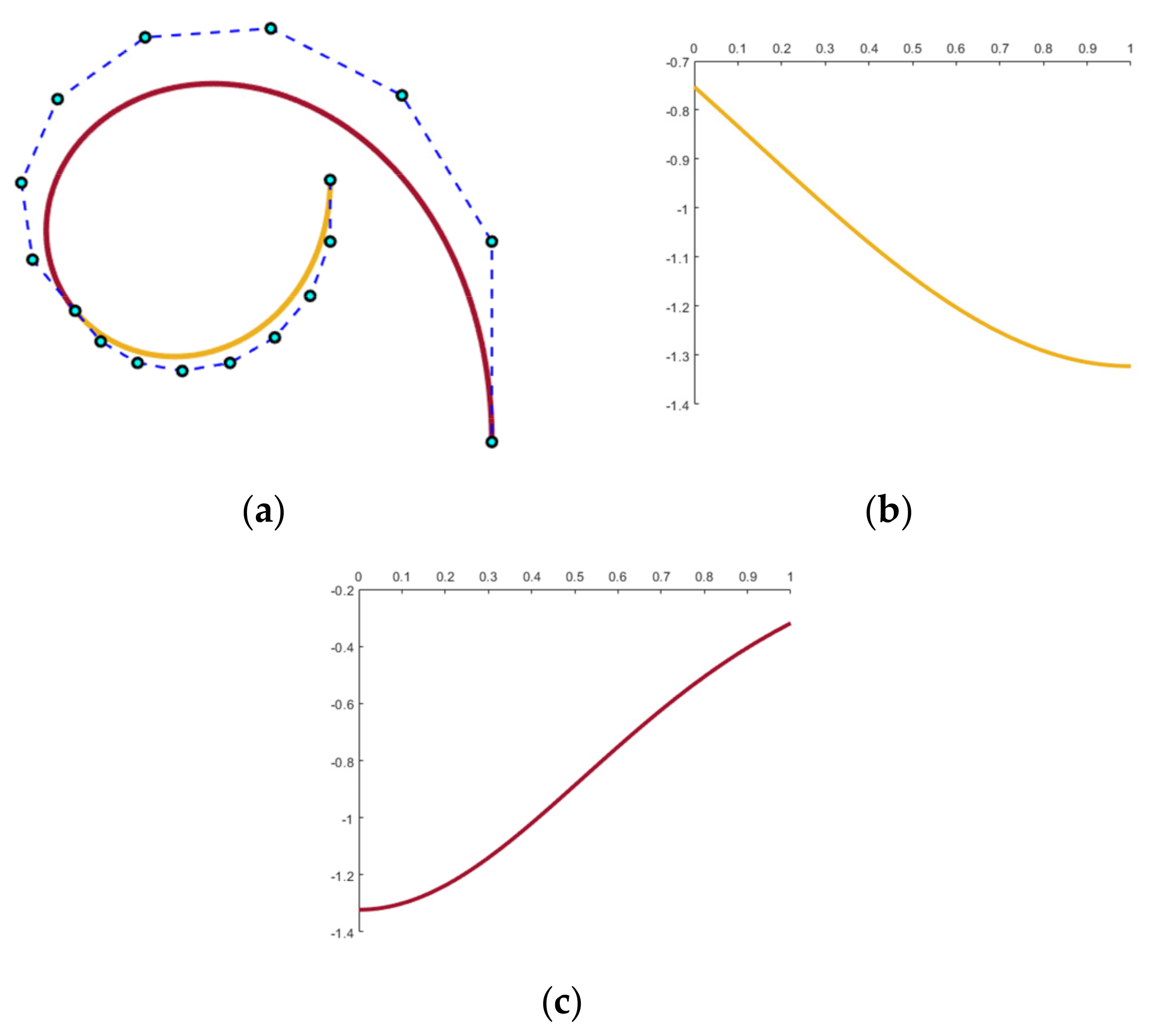
3.2. Subdivision at Curvature Extremum

As analyzed before, the typical Bézier curve has exactly one curvature extremum at $t^{\ast }=\frac{1-s\cos \theta }{s^2-2s\cos \theta +1}$ when $s\cdot \cos \theta <1$ ($s\ge 1$) or $s>\cos \theta$ ($0<s<1$); thus we can subdivide it into two Bézier curves with monotonic curvature (see Figure 10). This subsection will show that these subdivided segments are still typical curves. For the first segment, the scale factor $s_1$ and rotation angle ${\theta }_1$ of the new transformation matrix ${\mathit{M}}_1^{}$ satisfy $s_1=\cos {\theta }_1$, while for the second segment, $s_2\cos {\theta }_2=1$.

By subdividing the typical Bézier curve at $t^{\ast }$ we obtain two new transformation matrices ${\mathit{M}}_1^{}$ and ${\mathit{M}}_2^{}$, which can be expressed as

$${\mathit{M}}_1=\left(1-t^{\ast }\right)\mathit{I}+t^{\ast }\mathit{M}$$

(18)

$${\mathit{M}}_2={\left(t^{\ast }\mathit{I}+\left(1-t^{\ast }\right){\mathit{M}}^{-1}\right)}^{-1}$$

(19)

where ${\mathit{M}}^{-1}$ means the inverse of $\mathit{M}$. By expanding Equation (18) we get

$$\begin{array}{ll}{\mathit{M}}_1& =\left(\begin{array}{cc}1-t^{\ast }& 0\\ 0& 1-t^{\ast }\end{array}\right)+t^{\ast }\cdot s\cdot \left(\begin{array}{cc}\cos \theta & -\sin \theta \\ \sin \theta & \cos \theta \end{array}\right)\\ & =\left(\begin{array}{cc}1-t^{\ast }+t^{\ast }s\cos \theta & -t^{\ast }s\sin \theta \\ t^{\ast }s\sin \theta & 1-t^{\ast }+t^{\ast }s\cos \theta \end{array}\right)\end{array}$$

By substituting $t^{\ast }=\frac{1-s\cos \theta }{s^2-2s\cos \theta +1}$ into it, we then obtain

$${\mathit{M}}_1=\left(\begin{array}{cc}\frac{s^2{\sin }^2\theta }{s^2-2s\cos \theta +1}& -\frac{s\sin \theta -s^2\sin \theta \cos \theta }{s^2-2s\cos \theta +1}\\ \frac{s\sin \theta -s^2\sin \theta \cos \theta }{s^2-2s\cos \theta +1}& \frac{s^2{\sin }^2\theta }{s^2-2s\cos \theta +1}\end{array}\right)$$

Finally, it can be reorganized as

$${\mathit{M}}_1=\sigma \left(\begin{array}{cc}\sigma & -\sqrt{1-{\sigma }^2}\\ \sqrt{1-{\sigma }^2}& \sigma \end{array}\right)$$

(20)

where $\sigma =\frac{\left|s\sin \theta \right|}{\sqrt{s^2-2s\cos \theta +1}}\in \left[0,1\right]$. Equation (20) indicates that the associated segment constructed by ${\mathit{M}}_1$ belongs to a typical curve with $s_1=\cos {\theta }_1=\sigma$, where $s_1\le 1$ and ${\theta }_1\in [-\pi /2,\pi /2]$.

For Equation (19), note that ${\mathit{M}}_{inv}=t^{\ast }\mathit{I}+\left(1-t^{\ast }\right){\mathit{M}}^{-1}$; thus we have

$$\begin{array}{ll}{\mathit{M}}_{inv}& =\left(\begin{array}{cc}{t}^{\ast }& 0\\ 0& t^{\ast }\end{array}\right)+\left(1-t^{\ast }\right)\cdot \frac{1}{s}\cdot \left(\begin{array}{cc}\cos \theta & \sin \theta \\ -\sin \theta & \cos \theta \end{array}\right)=\left(\begin{array}{cc}{t}^{\ast }+\left(1-t^{\ast }\right)\frac{\cos \theta }{s}& \left(1-t^{\ast }\right)\frac{\sin \theta }{s}\\ -\left(1-t^{\ast }\right)\frac{\sin \theta }{s}& t^{\ast }+\left(1-t^{\ast }\right)\frac{\cos \theta }{s}\end{array}\right)\\ & =\left(\begin{array}{cc}\frac{{\sin }^2\theta }{s^2-2s\cos \theta +1}& \frac{\left(s-\cos \theta \right)\sin \theta }{s^2-2s\cos \theta +1}\\ -\frac{\left(s-\cos \theta \right)\sin \theta }{s^2-2s\cos \theta +1}& \frac{{\sin }^2\theta }{s^2-2s\cos \theta +1}\end{array}\right)\end{array}$$

Then, we obtain

$${\mathit{M}}_{inv}=\tau \left(\begin{array}{cc}\tau & \sqrt{1-{\tau }^2}\\ -\sqrt{1-{\tau }^2}& \tau \end{array}\right)$$

where $\tau =\frac{\left|\sin \theta \right|}{\sqrt{s^2-2s\cos \theta +1}}\in \left[0,1\right]$. Now we can obtain

$${\mathit{M}}_2={\left({\mathit{M}}_{inv}\right)}^{-1}=\frac{1}{\tau }\left(\begin{array}{cc}\tau & -\sqrt{1-{\tau }^2}\\ \sqrt{1-{\tau }^2}& \tau \end{array}\right)$$

(21)

Equation (21) indicates that the associated segment constructed by ${\mathit{M}}_2$ belongs to a typical curve with $\frac{1}{s_2}=\cos {\theta }_2=\tau$, where $s_2\ge 1$ and ${\theta }_2\in [-\pi /2,\pi /2]$.

Here we show two examples to demonstrate the subdivision results of typical Bézier curves. The first example is given for the case $s\cdot \cos \theta <1$ ($s\ge 1$) with $\Delta {\mathit{b}}_0^{}={\left[0,-1\right]}^{\mathit{T}}$, $k=8$ and $\mathit{M}=1.1\cdot \left(\begin{array}{cc}\cos \left(-2\pi /7\right)& -\sin \left(-2\pi /7\right)\\ \sin \left(-2\pi /7\right)& \cos \left(-2\pi /7\right)\end{array}\right)$ (Figure 11), the minimal curvature occurs at $t^{\ast }=0.3747$. After subdivision at $t^{\ast }$, we get ${\mathit{M}}_1=0.9393\cdot \left(\begin{array}{cc}0.9393& 0.3431\\ -0.3431& 0.9393\end{array}\right)$ and ${\mathit{M}}_2=1.7111\cdot \left(\begin{array}{cc}0.8539& 0.5204\\ -0.5204& 0.8539\end{array}\right)$ for each segment. Figure 12 illustrates these two typical curves in different colors.

The original data of the second example are given by $\Delta {\mathit{b}}_0^{}={\left[1,-1\right]}^{\mathit{T}}$, $k=6$ and $\mathit{M}=0.85\cdot \left(\begin{array}{cc}\cos \left(\pi /3\right)& -\sin \left(\pi /3\right)\\ \sin \left(\pi /3\right)& \cos \left(\pi /3\right)\end{array}\right)$ for the case $s>\cos \theta$ ($0<s<1$), the curvature extremum corresponds to $t^{\ast }=0.6590$ (Figure 13). After subdivision at $t^{\ast }$, we get ${\mathit{M}}_1=0.7881\cdot \left(\begin{array}{cc}0.7881& -0.6156\\ 0.6156& 0.7881\end{array}\right)$ and ${\mathit{M}}_2=1.0786\cdot \left(\begin{array}{cc}0.9271& -0.3747\\ 0.3747& 0.9271\end{array}\right)$ for each segment. Figure 14 illustrates these two typical curves in different colors.

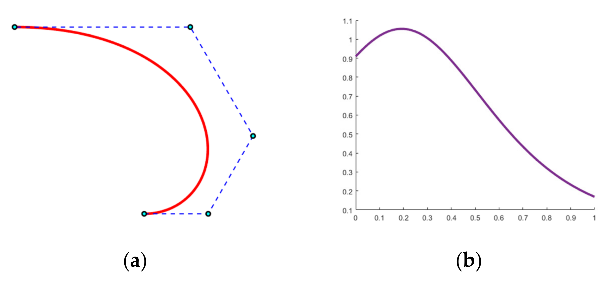
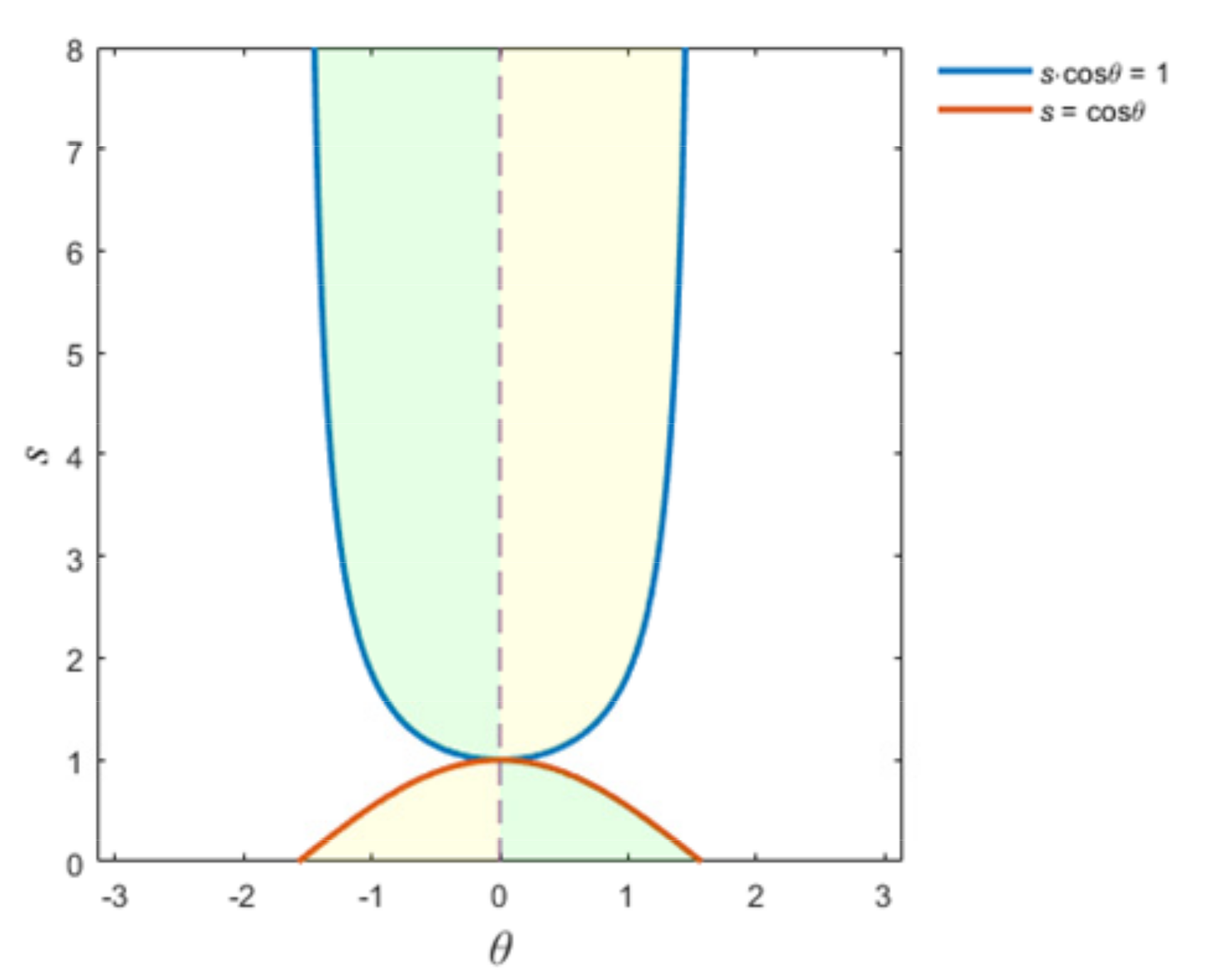
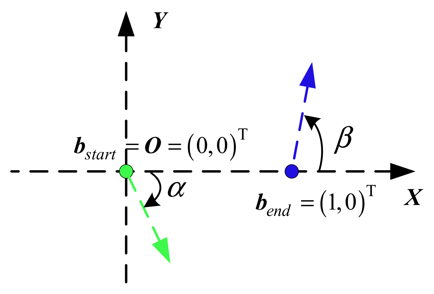
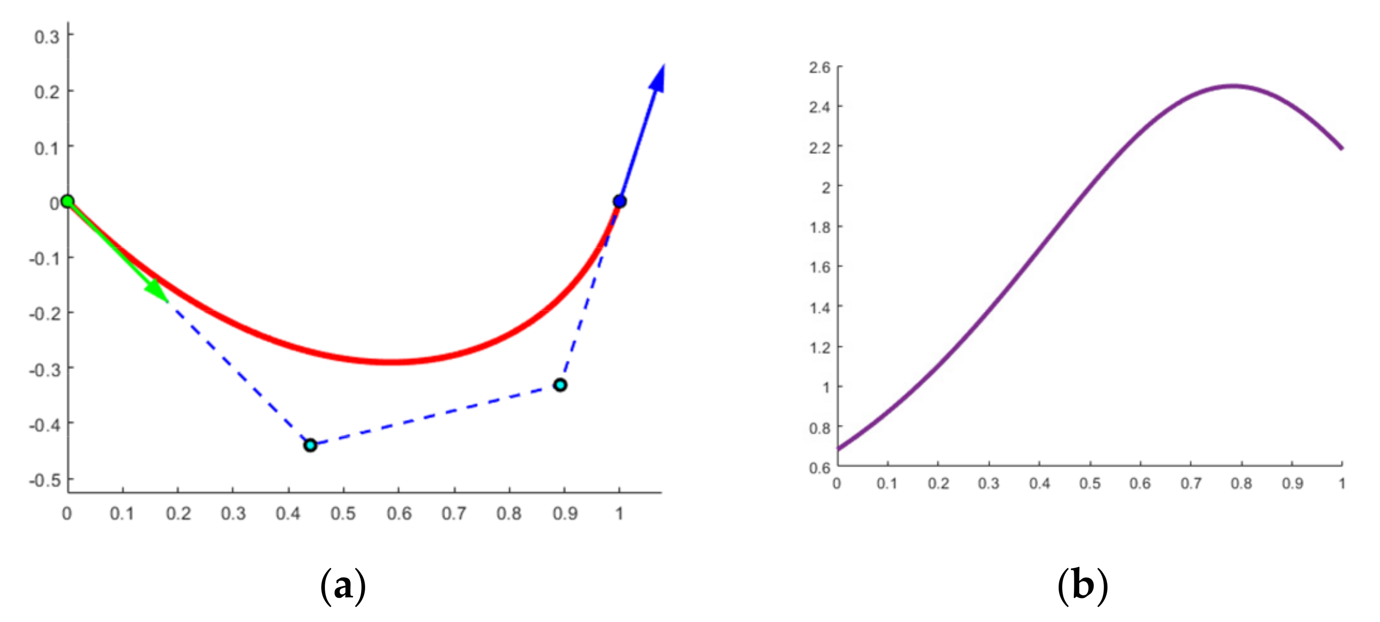
4. Solving G1 Interpolation with a Single Typical Bézier Curve

4.1. A Normalized form for G1 Interpolation

The aim of G1 interpolation is to construct a fairing curve matching given positions and associated tangents at a pair of endpoints. ${\mathit{b}}_{start}^{}$ is the start endpoint and ${\mathit{b}}_{end}^{}$ is the end point. Since the geometric properties of Bézier curves are invariant under affine transformation, we can set ${\mathit{b}}_{start}^{}$ at the origin and ${\mathit{b}}_{end}^{}$ at ${\left(1,0\right)}^{\mathrm{T}}$ by a pre-process, with the angle of associated tangents noted as $\alpha$ ($-\pi <\alpha <\pi$) and $\beta$ ($-\pi <\beta <\pi$) (Figure 15); we call this normalized form. The limitation of angular values is mainly for appearance, which requires the angular difference between two tangents to be less than $2\pi$ as Benjamin does for shape completion in ref [19], i.e., $0<\left|\beta -\alpha \right|<2\pi$.

In this section we provide sufficient conditions for G1 interpolation to have a typical Bézier curve solution under arbitrary degree. The G1 interpolation problem with a typical Bézier curve solution is equivalent to that where the following nonlinear system

$${\displaystyle \sum _{i=1}^k‖\Delta {\mathit{b}}_0^{}‖\cdot s^{i-1}\cdot \cos \left(\alpha +\left(i-1\right)\cdot \theta \right)=1}$$

(22)

$${\displaystyle \sum _{i=1}^k‖\Delta {\mathit{b}}_0^{}‖\cdot s^{i-1}\cdot \sin \left(\alpha +\left(i-1\right)\cdot \theta \right)=0}$$

(23)

has positive roots $s>0$ and $‖\Delta {\mathit{b}}_0^{}‖>0$, where $\theta =\left(\beta -\alpha \right)/\left(k-1\right)$. The interpolatory curve will have at most one curvature extremum.

4.2. Sufficient Condition for G1 Interpolation with Typical Bézier Curve Solution

Theorem 2.

If the given angles satisfy $-\pi /2<\alpha <0<\beta <\pi /2$ or $-\pi /2<\beta <0<\alpha <\pi /2$, then there exists a typical Bézier curve solution for the corresponding G1 interpolation problem for any degree $k\ge 2$.

Proof. 

In fact, these two cases are symmetric about the X-axis, so we only need to verify one of them. Here, we choose the case of $-\pi /2<\alpha <0<\beta <\pi /2$ (see Figure 15). We can simplify Equation (23) as the following equation with respect to $s$:

$${\displaystyle \sum _{i=1}^k{s}^{i-1}\cdot \sin \left(\alpha +\left(i-1\right)\cdot \theta \right)=0}$$

(24)

When $-\pi /2<\alpha <0<\beta <\pi /2$, then $-\pi /2<\alpha \le \alpha +\left(i-1\right)\cdot \theta \le \alpha +\beta <\pi /2$, and the series of coefficients $\sin \left(\alpha +\left(i-1\right)\cdot \theta \right)$ will change sign exactly once; thus, there exists a positive root $s_r$ such that Equation (23) holds for arbitrary $‖\Delta {\mathit{b}}_0^{}‖$ by Descartes’ rule of signs [20]. Substituting $s_r$ into Equation (22), we get

$${‖\Delta {\mathit{b}}_0^{}‖}_r=\frac{1}{{\displaystyle \sum _{i=1}^k\cdot s_r{}^{i-1}\cdot \cos \left(\alpha +\left(i-1\right)\cdot \theta \right)}}$$

(25)

Since $s_r>0$ and $\cos \left(\alpha +\left(i-1\right)\cdot \theta \right)>0$ always holds for $i=1,2,\dots ,k$, then ${‖\Delta {\mathit{b}}_0^{}‖}_r>0$. This means that $s_r>0$ and ${‖\Delta {\mathit{b}}_0^{}‖}_r>0$ such that Equations (22) and (23) hold, i.e., the corresponding G1 interpolation has a typical Bézier curve solution for $k\ge 2$. □

Theorem 2 indicates that to guarantee a typical Bézier curve solution for an arbitrary degree, the two tangents in the G1 interpolation problem should be located on the opposite side of the line formed by two endpoints, and each tangent should not deviate more than $\pi /2$ from the line.

We take $k=3$ of typical Bézier curves as an example in the following part to realize G1 interpolation in normalized form. The values of $s_r$ and ${‖\Delta {\mathit{b}}_0^{}‖}_r$ can be easily obtained because Equations (22) and (23) are degenerated to quadratic equations.

The boundary constraints of the first example are given as $\alpha =-\pi /4$ and $\beta =2\pi /5$ (see Figure 16), which belong to $-\pi /2<\alpha <0<\beta <\pi /2$. The green point-tangent pair and blue pair are the starting constraints and the ending constraints, respectively.

The second boundary constraints satisfy $-\pi /2<\beta <0<\alpha <\pi /2$ with $\alpha =\pi /3$ and $\beta =-\pi /3$ (Figure 17). The point-tangent pairs are on a circular arc, and the interpolation curve will be symmetric with $s_r=1$.

Theorem 2 presents a sufficient condition, but that does not mean there is no typical Bézier curve solution while the values of angles exceed the limitation of $\pm \pi /2$. In fact, as degree $k$ increases, the denominator of ${‖\Delta {\mathit{b}}_0^{}‖}_r=\frac{1}{{\displaystyle \sum _{i=1}^k\cdot s_r{}^{i-1}\cdot \cos \left(\alpha +\left(i-1\right)\cdot \theta \right)}}$ is more likely to be positive, for the number of positive terms will increase. However, the precise relationship between degree $k$ and the tangent angles requires further research.

5. Conclusions

Aesthetic curves play an important role in CAD and CAGD. It is important to realize monotonously varying curvature distribution or to control the number of curvature extrema to as few as possible. In this paper, we discuss the planar typical curves with one curvature extremum, and both geometric proof and algebraic solutions are provided. The parameter at the curvature extremum can be calculated directly from typical curves, which can help us determine the point with maximal or minimal curvature quickly and subdivide it into two typical curves with monotonic curvature. Typical Bézier curves are more likely to have a solution in G1 interpolation without the restriction of monotonic curvature, and we give a sufficient condition to guarantee the interpolation solution for arbitrary degrees.

Future work should apply typical Bézier curves to geometric interpolation, matching higher order such as G2 or G3 interpolation problems, and determine the relationship between positive solutions and degree k. Furthermore, the constant $s$ and $\theta$ for any typical curve limit the degree of freedom; thus, another aim is to realize Bézier curves with monotonic curvature using different values of $s$ or $\theta$.

References

1. Farin, G.; Sapidis, N. Curvature and the fairness of curves and surfaces. IEEE Comput. Graph. Appl. 1989, 9, 52–57. [Google Scholar] [CrossRef]
2. Farin, G. Curves and Surfaces for CAGD: A Practical Guide, 5th ed.; Morgan Kaufmann: Burlington, MA, USA, 2002. [Google Scholar]
3. Beeker, E. Smoothing of shapes designed with free-form surfaces. Comput.-Aided Des. 1986, 18, 224–232. [Google Scholar] [CrossRef]
4. Wang, Y.; Zhao, B.; Zhang, L.; Xu, J.; Wang, K.; Wang, S. Designing fair curves using monotone curvature pieces. Comput. Aided Geom. Des. 2004, 21, 515–527. [Google Scholar] [CrossRef]
5. Sapidis, N.S.; Frey, W.H. Controlling the curvature of a quadratic Bézier curve. Comput. Aided Geom. Des. 1992, 9, 85–91. [Google Scholar] [CrossRef]
6. Mineur, Y.; Lichah, T.; Castelain, J.M.; Giaume, H. A shape controled fitting method for Bézier curves. Comput. Aided Geom. Des. 1998, 15, 879–891. [Google Scholar] [CrossRef]
7. Farin, G. Class A Bézier curves. Comput. Aided Geom. Des. 2006, 23, 573–581. [Google Scholar] [CrossRef]
8. Cao, J.; Wang, G. A note on Class a Bézier curves. Comput. Aided Geom. Des. 2008, 25, 523–528. [Google Scholar] [CrossRef]
9. Wang, A.; Zhao, G. Counter examples of “Class A Bézier curves”. Comput. Aided Geom. Des. 2018, 61, 6–8. [Google Scholar] [CrossRef]
10. Cantón, A.; Fernández-Jambrina, L.; Vázquez-Gallo, M.J. Curvature of planar aesthetic curves. J. Comput. Appl. Math. 2021, 381, 113042. [Google Scholar] [CrossRef]
11. Tong, W.; Chen, M. A sufficient condition for 3D typical curves. Comput. Aided Geom. Des. 2021, 87, 101991. [Google Scholar] [CrossRef]
12. Wang, A.; Zhao, G.; Hou, F. Constructing Bézier curves with monotone curvature. J. Comput. Appl. Math. 2019, 355, 1–10. [Google Scholar] [CrossRef]
13. Wang, A.; He, C.; Hou, F.; Cai, Z.; Zhao, G. Designing planar cubic B-spline curves with monotonic curvature for curve interpolation. Comput. Vis. Media 2020, 6, 349–354. [Google Scholar] [CrossRef]
14. Levien, R.; Séquin, C.H. Interpolating splines: Which is the fairest of them all? Comput.-Aided Des. Appl. 2009, 6, 91–102. [Google Scholar] [CrossRef] [Green Version]
15. Yan, Z.; Schiller, S.; Wilensky, G.; Carr, N.; Schaefer, S. K-curves: Interpolation at local maximum curvature. ACM Trans. Graph. (TOG) 2017, 36, 1–7. [Google Scholar] [CrossRef]
16. Yan, Z.; Schiller, S.; Schaefer, S. Circle reproduction with interpolatory curves at local maximal curvature points. Comput. Aided Geom. Des. 2019, 72, 98–110. [Google Scholar] [CrossRef]
17. Miura, K.T.; Gobithaasan, R.U.; Salvi, P.; Wang, D.; Sekine, T.; Usuki, S.; Inoguchi, J.; Kajiwara, K. ϵκ-Curves: Controlled local curvature extremum. Vis. Comput. 2021, 1–16. [Google Scholar] [CrossRef]
18. Yuksel, C. A Class of C 2 Interpolating Splines. ACM Trans. Graph. (TOG) 2020, 39, 1–14. [Google Scholar] [CrossRef]
19. Kimia, B.B.; Frankel, I.; Popescu, A.M. Euler spiral for shape completion. Int. J. Comput. Vis. 2003, 54, 159–182. [Google Scholar] [CrossRef]
20. Henrici, P. Applied and Computational Complex Analysis; Wiley: New York, NY, USA, 1988; Volume 1. [Google Scholar]
Figure 1. The construction of typical Bézier curves. (a) Control edges are designed according to (a) Δ b i = M i Δ b 0 ; (b) b i b i + 1 1 = b i + 1 b i + 2 , b i b i + 2 1 = b i + 2 b i + 3 ; (c) P ( t ) and P ( t ) are generated by the de Casteljau algorithm.
Mathematics 09 02148 g001
Figure 2. The domain of b i + 1 1 for s cos θ < 1 ( s 1 , θ [ 0 , π ] ) in the local coordinate system.
Mathematics 09 02148 g002
Figure 3. Acute triangle b i b h b i , k 3 1 b i + 1 , k 3 1 , where b h corresponds to parameter t .
Mathematics 09 02148 g003
Figure 4. A typical Bézier curve with k = 4 when s cos θ < 1 ( s 1 ). (a) s = 1.4 , θ = π / 3 and Δ b 0 = 1 , 0 T ; (b) curvature plot.
Mathematics 09 02148 g004
Figure 5. A typical Bézier curve with k = 5 when s > cos θ ( 0 < s < 1 ). (a) s = 0.9 , θ = π / 4 and Δ b 0 = 1 , 0 T ; (b) curvature plot.
Mathematics 09 02148 g005
Figure 6. Transformation effect of matrix M and T t .
Mathematics 09 02148 g006
Figure 7. The de Casteljau algorithm of P ( t ) .
Mathematics 09 02148 g007
Figure 8. Regions for curvature variation of typical Bézier curves. Curvature decreases in the light yellow area and increases in the light green area. While in the white area, curvature variation is not monotonous and possesses only one extremum. Specifically, for θ < 0 there is a local minimum and for θ > 0 there is a local maximum.
Mathematics 09 02148 g008
Figure 9. Symmetric typical Bézier curve with k = 10 when s = 1 . (a) θ = π / 6 and Δ b 0 = 1 , 1 T ; (b) symmetric curvature plot with a local minimum at t = 0.5 .
Mathematics 09 02148 g009
Figure 10. Subdivision of a cubic typical Bézier curve at curvature extremum.
Mathematics 09 02148 g010
Figure 11. Typical Bézier curve with degree k = 8 for s cos θ < 1 ( s 1 ). (a) Transformation matrix M = 1.1 cos 2 π / 7 sin 2 π / 7 sin 2 π / 7 cos 2 π / 7 ; point with curvature extremum is represented by yellow dot; (b) curvature plot has a minimum at t = 0.3747 .
Mathematics 09 02148 g011
Figure 12. Results under subdivision. (a) Two typical curve segments join at t ; (b) first segment has decreasing curvature variation; (c) second segment has increasing curvature variation.
Mathematics 09 02148 g012
Figure 13. Typical Bézier curve with degree k = 6 for s > cos θ ( 0 < s < 1 ). (a) Transformation matrix M = 0.85 cos π / 3 sin π / 3 sin π / 3 cos π / 3 ; point with curvature extremum is represented by yellow dot; (b) curvature plot has a maximum at t = 0.6590 .
Mathematics 09 02148 g013
Figure 14. Results under subdivision. (a) Two typical curve segments join at t ; (b) first segment has increasing curvature variation; (c) second segment has decreasing curvature variation.
Mathematics 09 02148 g014
Figure 15. The boundary constraints of G1 interpolation in normalized form.
Mathematics 09 02148 g015
Figure 16. Cubic typical Bézier curve solution for π / 2 < α < 0 < β < π / 2 . (a) s r = 0.7482 , Δ b 0 r = 0.6220 ; (b) corresponding curvature plot.
Mathematics 09 02148 g016
Figure 17. Cubic typical Bézier curve solution for π / 2 < β < 0 < α < π / 2 . (a) s r = 1 , Δ b 0 r = 0.5 ; (b) corresponding curvature plot.
Mathematics 09 02148 g017
Publisher’s Note: MDPI stays neutral with regard to jurisdictional claims in published maps and institutional affiliations.