
Reversible Data Hiding Based on Pixel-Value-Ordering and Prediction-Error Triplet Expansion


Abstract
:1. Introduction
2. Related Works
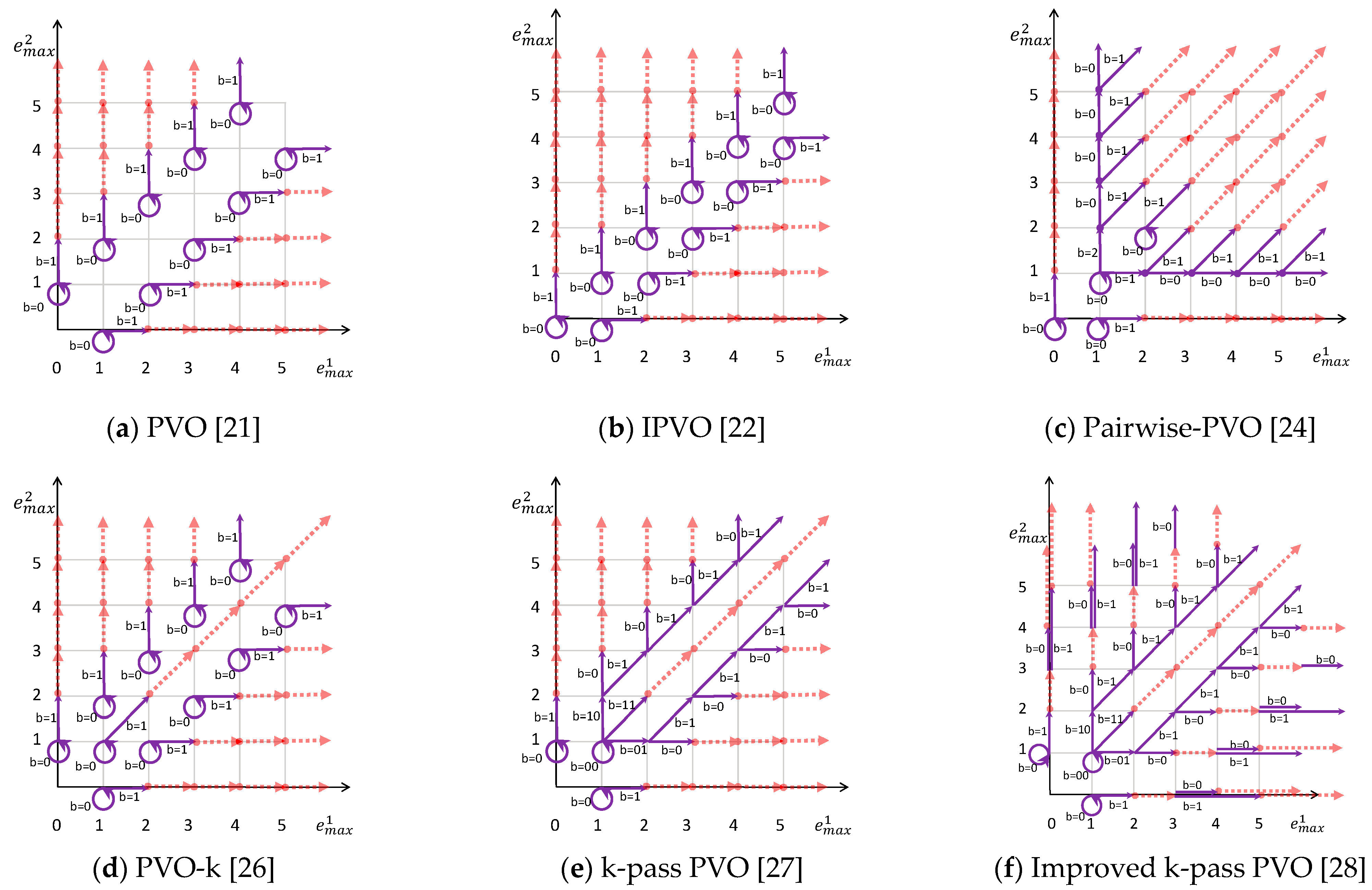
2.1. PVO
2.2. IPVO
2.3. Pairwise-PVO
2.4. Other Typical PVO-Based Schemes
3. Proposed Scheme
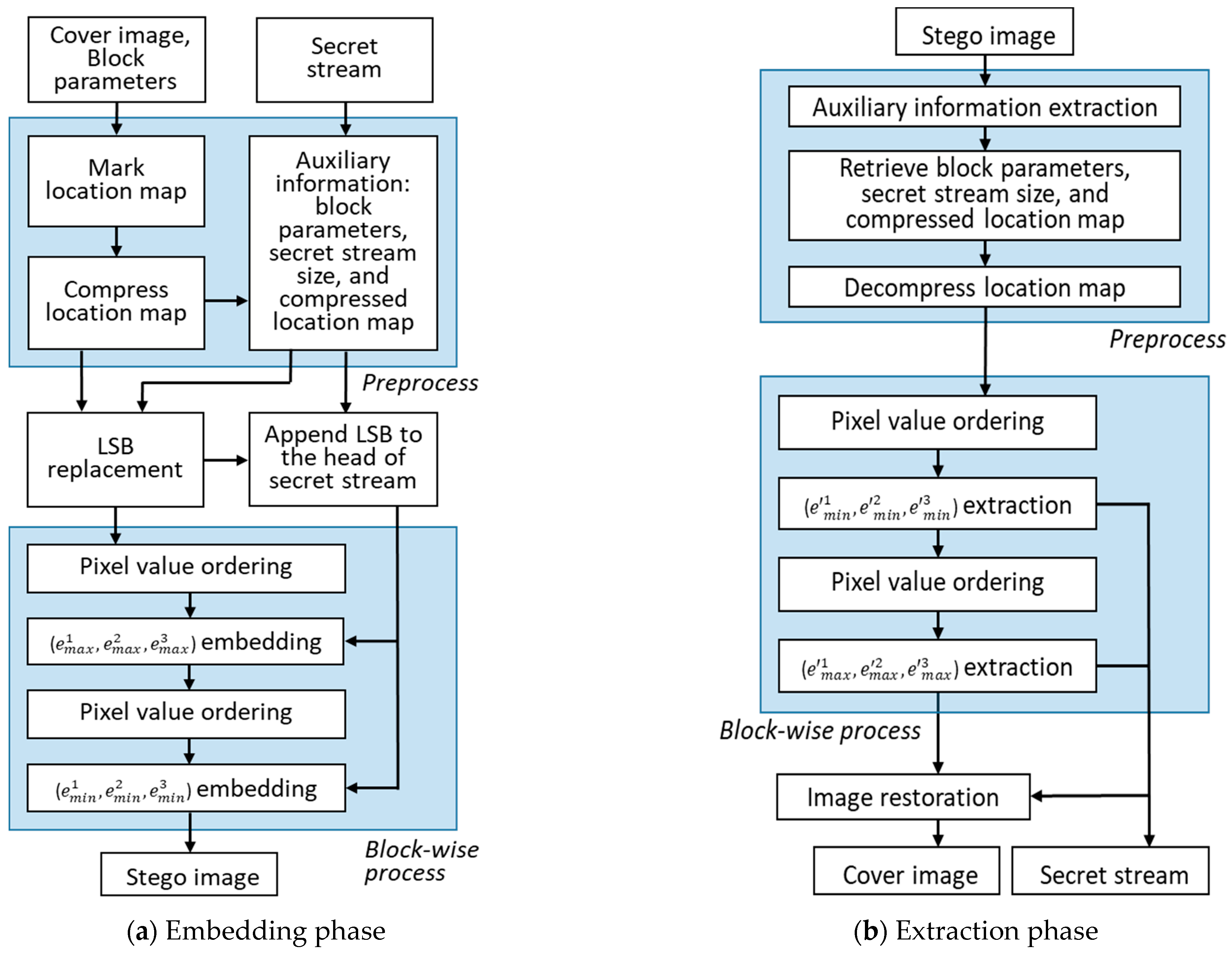
3.1. Framework and Preprocess
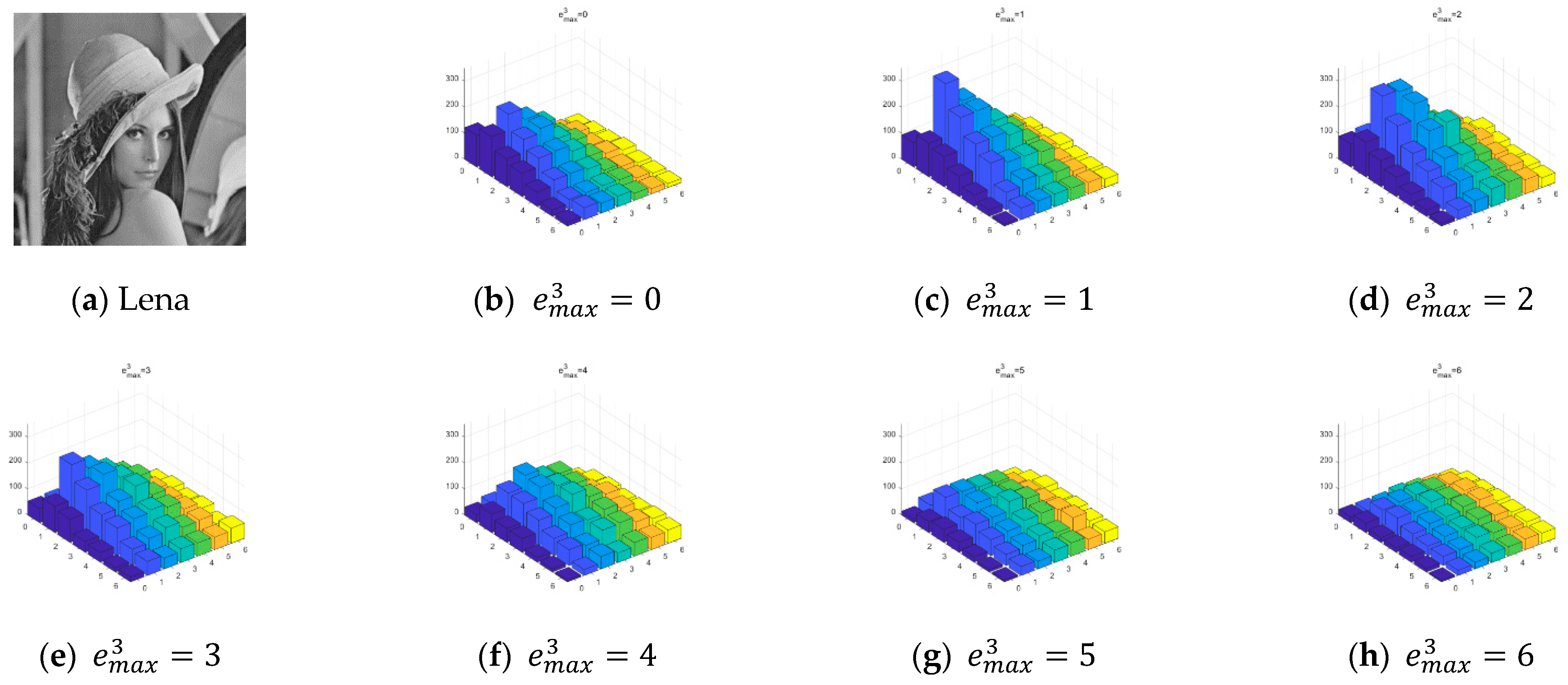
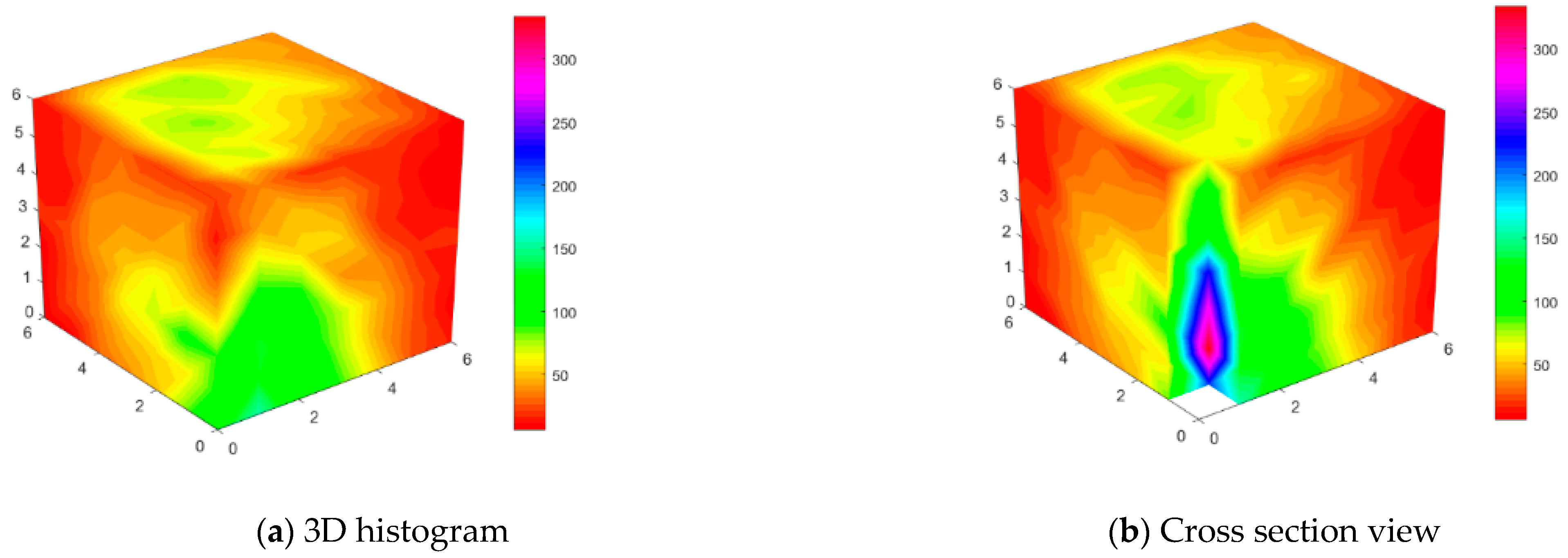
3.2. 3D State Transition Map
- For the 0-th layer ():
- :
- :
- :
- For the -th (except for 0) layer ():
- :
- :
- :
- :
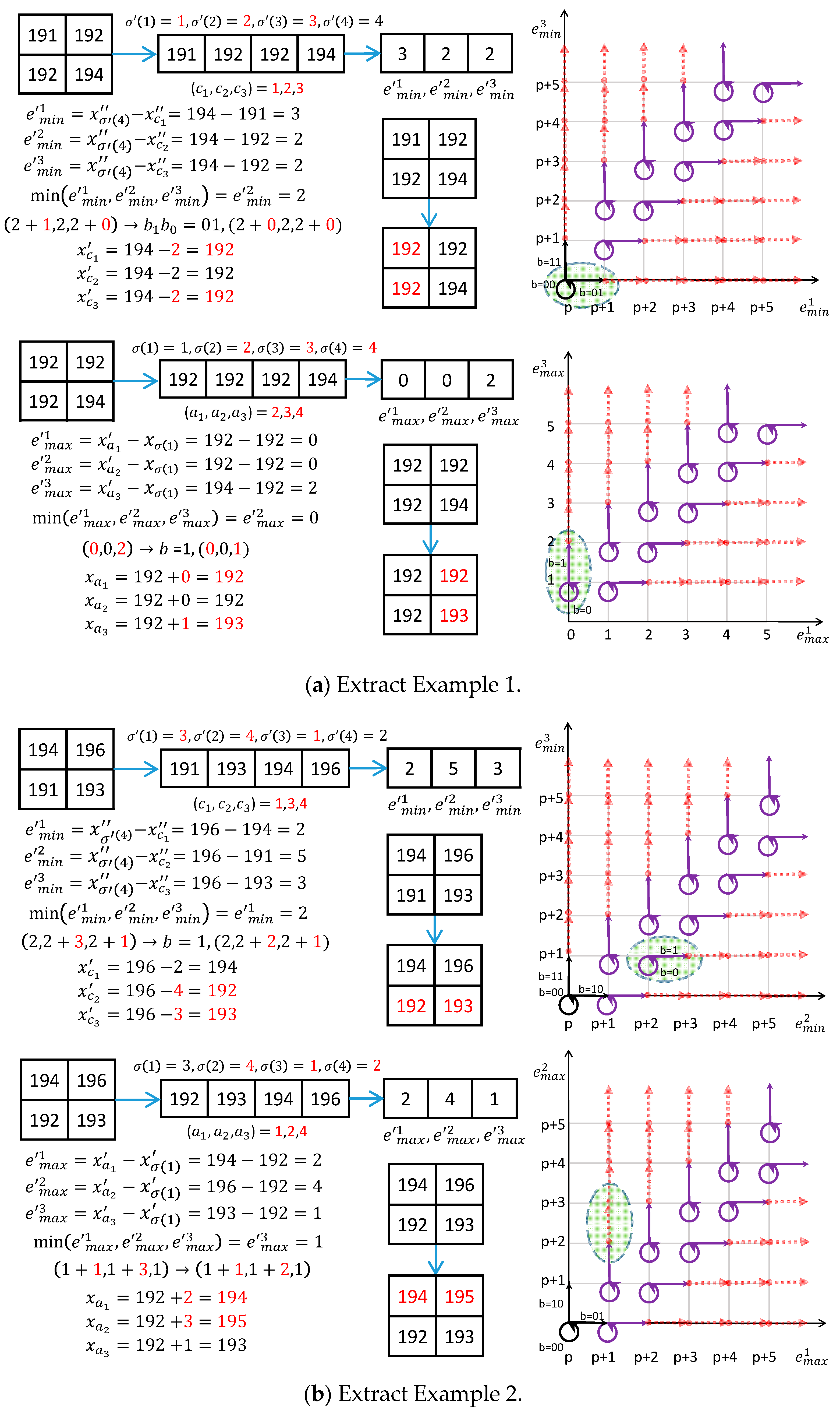
3.3. Examples of Secret Data Embedding
3.4. Data Extraction and Image Recovery
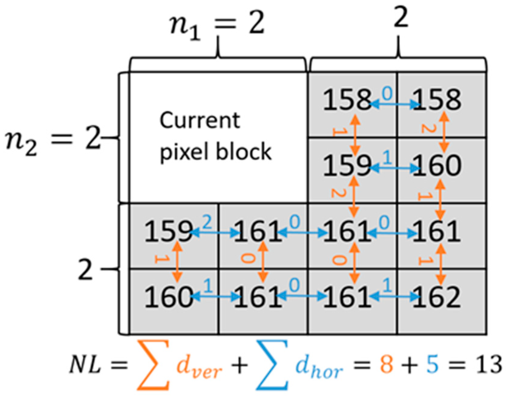
3.5. Complex Block Exclusion
4. Experimental Results and Comparisons
4.1. Experimental Results
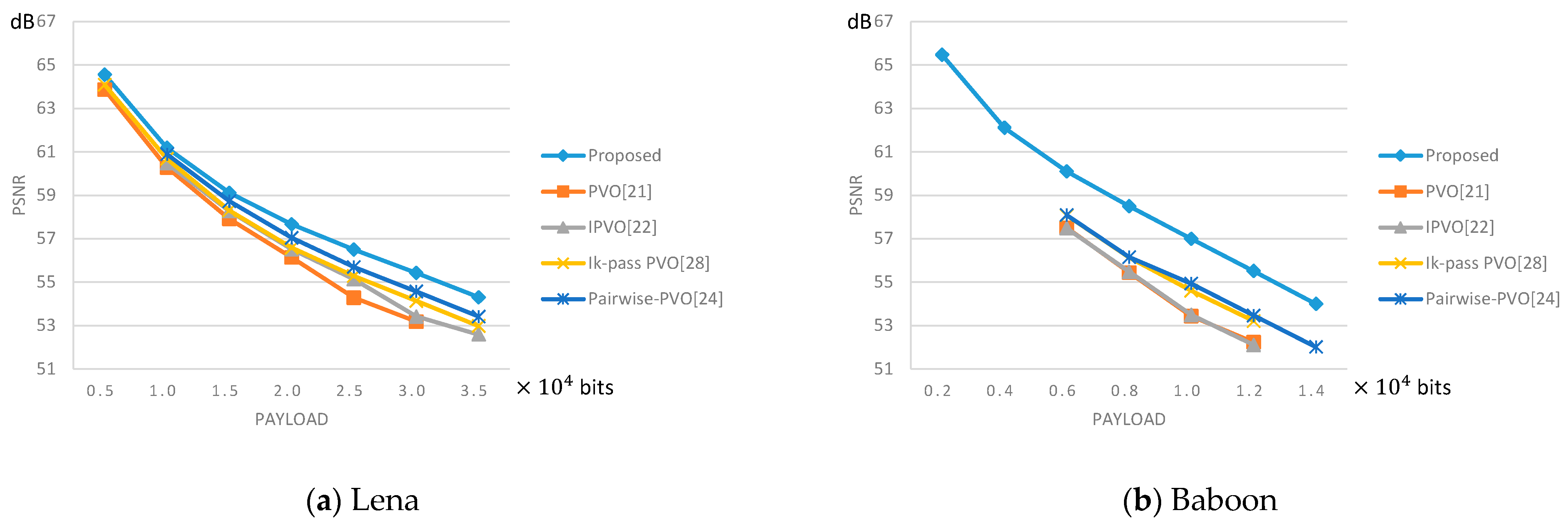
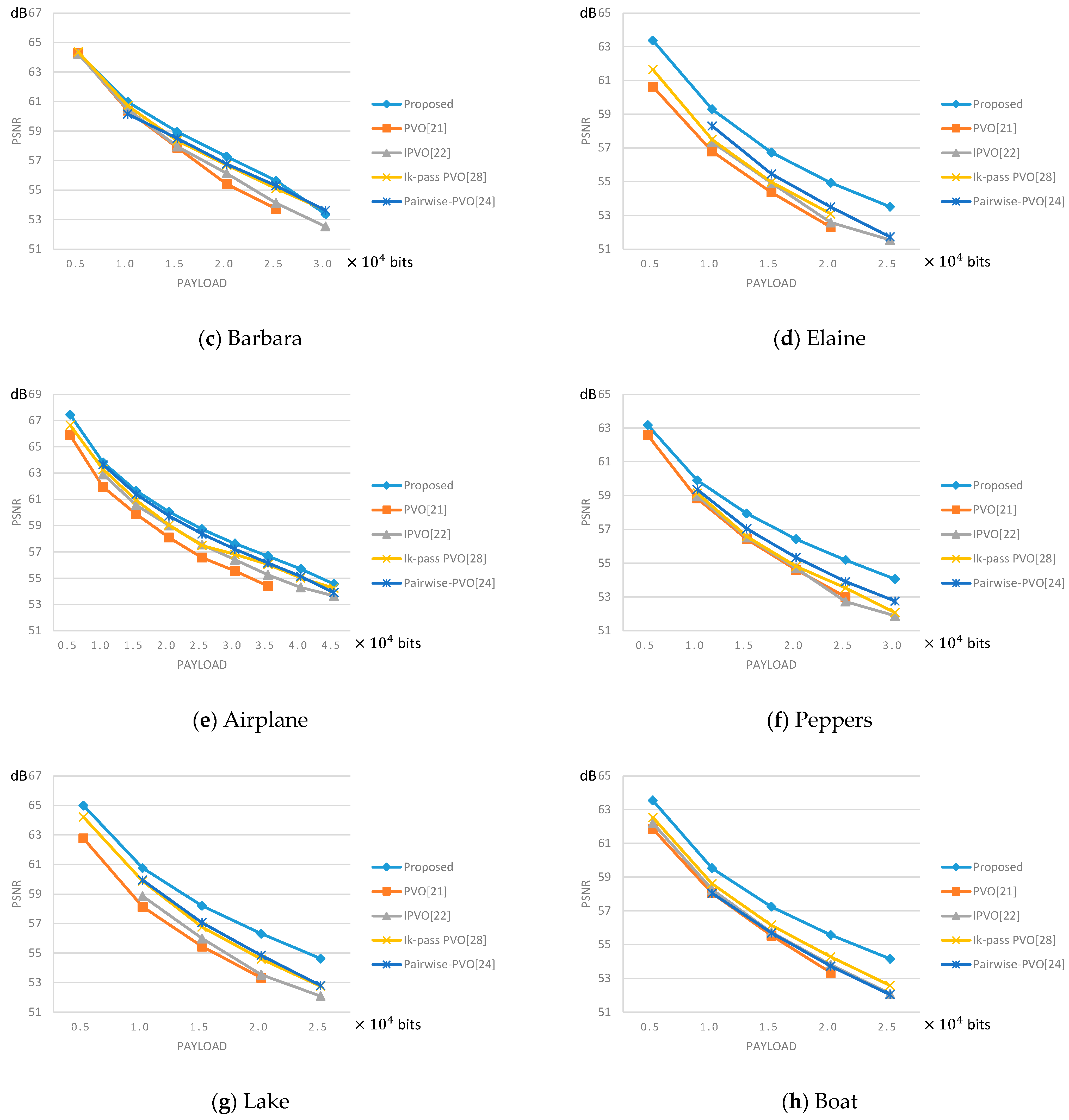
4.2. Comparisons
5. Conclusions
Author Contributions
Funding
Institutional Review Board Statement
Informed Consent Statement
Data Availability Statement
Conflicts of Interest
References
- Chang, C.-C. Adversarial Learning for Invertible Steganography. IEEE Access 2020, 8, 198425–198435. [Google Scholar] [CrossRef]
- Chang, C.-C.; Li, C.-T.; Shi, Y.-Q. Privacy-Aware Reversible Watermarking in Cloud Computing Environments. IEEE Access 2018, 6, 70720–70733. [Google Scholar] [CrossRef]
- Chi, H.; Chang, C.-C.; Liu, Y. An SMVQ Compressed Data Hiding Scheme Based on Multiple Linear Regression Prediction. Connect. Sci. 2020, 1–20. [Google Scholar] [CrossRef]
- Chen, K.-M. High Capacity Reversible Data Hiding Based on the Compression of Pixel Differences. Mathematics 2020, 8, 1435. [Google Scholar] [CrossRef]
- Yu, C.; Ye, C.; Zhang, X.; Tang, Z.; Zhan, S. Separable Reversible Data Hiding in Encrypted Image Based on Two-Dimensional Permutation and Exploiting Modification Direction. Mathematics 2019, 7, 976. [Google Scholar] [CrossRef] [Green Version]
- Sun, Y.; Lu, Y.; Chen, J.; Zhang, W.; Yan, X. Meaningful Secret Image Sharing Scheme with High Visual Quality Based on Natural Steganography. Mathematics 2020, 8, 1452. [Google Scholar] [CrossRef]
- Chang, C.C.; Liu, Y.; Nguyen, T.S. A Novel Turtle Shell Based Scheme for Data Hiding. In Proceedings of the Tenth International Conference on Intelligent Information Hiding and Multimedia Signal Processing, Kitakyushu, Japan, 27–29 August 2014; pp. 89–93. [Google Scholar] [CrossRef]
- Qin, J.; Wang, J.; Tan, Y.; Huang, H.; Xiang, X.; He, Z. Coverless Image Steganography Based on Generative Adversarial Network. Mathematics 2020, 8, 1394. [Google Scholar] [CrossRef]
- Alattar, A.M. Reversible Watermark Using the Difference Expansion of a Generalized Integer Transform. IEEE Trans. Image Process. 2004, 13, 1147–1156. [Google Scholar] [CrossRef]
- Hu, Y.; Lee, H.-K.; Li, J. DE-Based Reversible Data Hiding With Improved Overflow Location Map. IEEE Trans. Circuits Syst. Video Technol. 2009, 19, 250–260. [Google Scholar] [CrossRef]
- Tian, J. Reversible Data Embedding Using a Difference Expansion. IEEE Trans. Circuits Syst. Video Technol. 2003, 13, 890–896. [Google Scholar] [CrossRef] [Green Version]
- Li, X.; Li, B.; Yang, B.; Zeng, T. General Framework to Histogram-Shifting-Based Reversible Data Hiding. IEEE Trans. Image Process. 2013, 22, 2181–2191. [Google Scholar] [CrossRef]
- Ni, Z.; Shi, Y.-Q.; Ansari, N.; Su, W. Reversible Data Hiding. IEEE Trans. Circuits Syst. Video Technol. 2006, 16, 354–362. [Google Scholar] [CrossRef]
- Tsai, P.; Hu, Y.-C.; Yeh, H.-L. Reversible Image Hiding Scheme Using Predictive Coding and Histogram Shifting. Signal Process. 2009, 89, 1129–1143. [Google Scholar] [CrossRef]
- Dragoi, I.-C.; Coltuc, D. Local-Prediction-Based Difference Expansion Reversible Watermarking. IEEE Trans. Image Process. 2014, 23, 1779–1790. [Google Scholar] [CrossRef]
- Dragoi, I.-C.; Coltuc, D. Adaptive Pairing Reversible Watermarking. IEEE Trans. Image Process. 2016, 25, 2420–2422. [Google Scholar] [CrossRef]
- He, W.; Xiong, G.; Weng, S.; Cai, Z.; Wang, Y. Reversible Data Hiding Using Multi-Pass Pixel-Value-Ordering and Pairwise Prediction-Error Expansion. Inf. Sci. 2018, 467, 784–799. [Google Scholar] [CrossRef]
- Sachnev, V.; Kim, H.J.; Nam, J.; Suresh, S.; Shi, Y.Q. Reversible Watermarking Algorithm Using Sorting and Prediction. IEEE Trans. Circuits Syst. Video Technol. 2009, 19, 989–999. [Google Scholar] [CrossRef]
- Luo, L.; Chen, Z.; Chen, M.; Zeng, X.; Xiong, Z. Reversible Image Watermarking Using Interpolation Technique. IEEE Trans. Inf. Forensics Secur. 2010, 5, 187–193. [Google Scholar] [CrossRef]
- Ou, B.; Li, X.; Zhao, Y.; Ni, R.; Shi, Y.-Q. Pairwise Prediction-Error Expansion for Efficient Reversible Data Hiding. IEEE Trans. Image Process. 2013, 22, 5010–5021. [Google Scholar] [CrossRef] [PubMed]
- Li, X.; Li, J.; Li, B.; Yang, B. High-Fidelity Reversible Data Hiding Scheme Based on Pixel-Value-Ordering and Prediction-Error Expansion. Signal Process. 2013, 93, 198–205. [Google Scholar] [CrossRef]
- Peng, F.; Li, X.; Yang, B. Improved PVO-Based Reversible Data Hiding. Digit. Signal Process. 2014, 25, 255–265. [Google Scholar] [CrossRef]
- He, W.; Cai, Z.; Wang, Y. Flexible Spatial Location-Based PVO Predictor for High-Fidelity Reversible Data Hiding. Inf. Sci. 2020, 520, 431–444. [Google Scholar] [CrossRef]
- Ou, B.; Li, X.; Wang, J. High-Fidelity Reversible Data Hiding Based on Pixel-Value-Ordering and Pairwise Prediction-Error Expansion. J. Vis. Commun. Image Represent. 2016, 39, 12–23. [Google Scholar] [CrossRef] [Green Version]
- Zhang, T.; Li, X.; Qi, W.; Guo, Z. Location-Based PVO and Adaptive Pairwise Modification for Efficient Reversible Data Hiding. IEEE Trans. Inf. Forensics Secur. 2020, 15, 2306–2319. [Google Scholar] [CrossRef]
- Ou, B.; Li, X.; Zhao, Y.; Ni, R. Reversible Data Hiding Using Invariant Pixel-Value-Ordering and Prediction-Error Expansion. Signal Process. Image Commun. 2014, 29, 760–772. [Google Scholar] [CrossRef]
- He, W.; Zhou, K.; Cai, J.; Wang, L.; Xiong, G. Reversible Data Hiding Using Multi-Pass Pixel Value Ordering and Prediction-Error Expansion. J. Vis. Commun. Image Represent. 2017, 49, 351–360. [Google Scholar] [CrossRef]
- Weng, S.; Chen, Y.; Ou, B.; Chang, C.-C.; Zhang, C. Improved K-Pass Pixel Value Ordering Based Data Hiding. IEEE Access 2019, 7, 34570–34582. [Google Scholar] [CrossRef]


| Image | ||||||
|---|---|---|---|---|---|---|
| Lena | 59.51 | 60.26 | 60.20 | 61.05 | 61.18 | 61.42 |
| Baboon | 55.33 | 55.84 | 55.33 | 56.89 | 56.99 | 56.72 |
| Barbara | 59.65 | 60.01 | 59.68 | 60.97 | 60.98 | 61.28 |
| Elaine | 58.03 | 58.52 | 57.85 | 59.19 | 59.29 | 59.30 |
| Airplane | 62.63 | 63.07 | 62.97 | 63.73 | 63.80 | 63.63 |
| Peppers | 58.30 | 58.55 | 58.48 | 59.75 | 59.90 | 60.40 |
| Lake | 59.72 | 59.92 | 59.39 | 60.88 | 60.76 | 60.72 |
| Boat | 58.22 | 58.51 | 58.49 | 59.50 | 59.52 | 59.81 |
| Image | PSNR | Block Size | T |
|---|---|---|---|
| Airplane | 63.80 | 20 | |
| Baboon | 56.99 | 223 | |
| Barbara | 61.29 | 65 | |
| Boat | 59.82 | 106 | |
| Elaine | 59.29 | 97 | |
| Lake | 60.88 | 68 | |
| Lena | 61.57 | 70 | |
| Peppers | 60.55 | 105 |
| Image | Proposed | [21] | [22] | [24] | [27] | [28] |
|---|---|---|---|---|---|---|
| Lena | 61.18 | 60.28 | 60.47 | 60.90 | 60.64 | 60.68 |
| Baboon | 56.99 | 53.43 | 53.49 | 54.94 | 54.00 | 54.60 |
| Barbara | 60.98 | 60.39 | 60.48 | 60.14 | 60.37 | 60.72 |
| Elaine | 59.29 | 56.79 | 57.34 | 58.29 | 57.67 | 57.49 |
| Airplane | 63.80 | 61.95 | 62.90 | 63.63 | 63.45 | 63.28 |
| Peppers | 59.90 | 58.83 | 58.97 | 59.36 | 59.29 | 59.14 |
| Lake | 60.76 | 58.13 | 58.85 | 59.94 | 59.71 | 59.86 |
| Boat | 59.52 | 58.05 | 58.25 | 58.05 | 58.28 | 58.61 |
| Image | Proposed | [21] | [22] | [24] | [27] | [28] |
|---|---|---|---|---|---|---|
| Lena | 57.67 | 56.14 | 56.51 | 57.04 | 56.81 | 56.67 |
| Baboon | — | — | — | — | — | — |
| Barbara | 57.27 | 55.40 | 56.13 | 55.88 | 56.09 | 56.74 |
| Elaine | 54.93 | 52.31 | 52.58 | 53.50 | 53.08 | 53.14 |
| Airplane | 60.04 | 58.09 | 58.99 | 59.73 | 59.59 | 59.18 |
| Peppers | 56.42 | 54.61 | 54.71 | 55.34 | 55.10 | 54.97 |
| Lake | 56.31 | 53.32 | 53.54 | 54.84 | 54.53 | 54.66 |
| Boat | 55.57 | 53.34 | 53.81 | 53.72 | 54.07 | 54.27 |
Publisher’s Note: MDPI stays neutral with regard to jurisdictional claims in published maps and institutional affiliations. |
© 2021 by the authors. Licensee MDPI, Basel, Switzerland. This article is an open access article distributed under the terms and conditions of the Creative Commons Attribution (CC BY) license (https://creativecommons.org/licenses/by/4.0/).
Share and Cite
Chi, H.-X.; Horng, J.-H.; Chang, C.-C. Reversible Data Hiding Based on Pixel-Value-Ordering and Prediction-Error Triplet Expansion. Mathematics 2021, 9, 1703. https://doi.org/10.3390/math9141703
Chi H-X, Horng J-H, Chang C-C. Reversible Data Hiding Based on Pixel-Value-Ordering and Prediction-Error Triplet Expansion. Mathematics. 2021; 9(14):1703. https://doi.org/10.3390/math9141703
Chicago/Turabian StyleChi, Heng-Xiao, Ji-Hwei Horng, and Chin-Chen Chang. 2021. "Reversible Data Hiding Based on Pixel-Value-Ordering and Prediction-Error Triplet Expansion" Mathematics 9, no. 14: 1703. https://doi.org/10.3390/math9141703