
Nonlinear Differential Braking Control for Collision Avoidance During Lane Change


Abstract
:1. Introduction
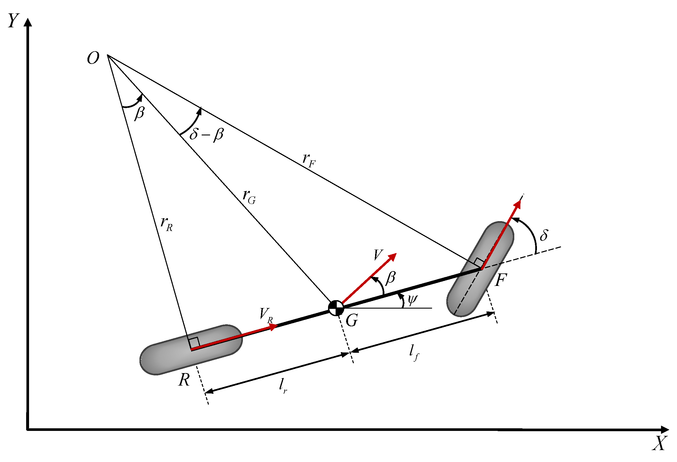
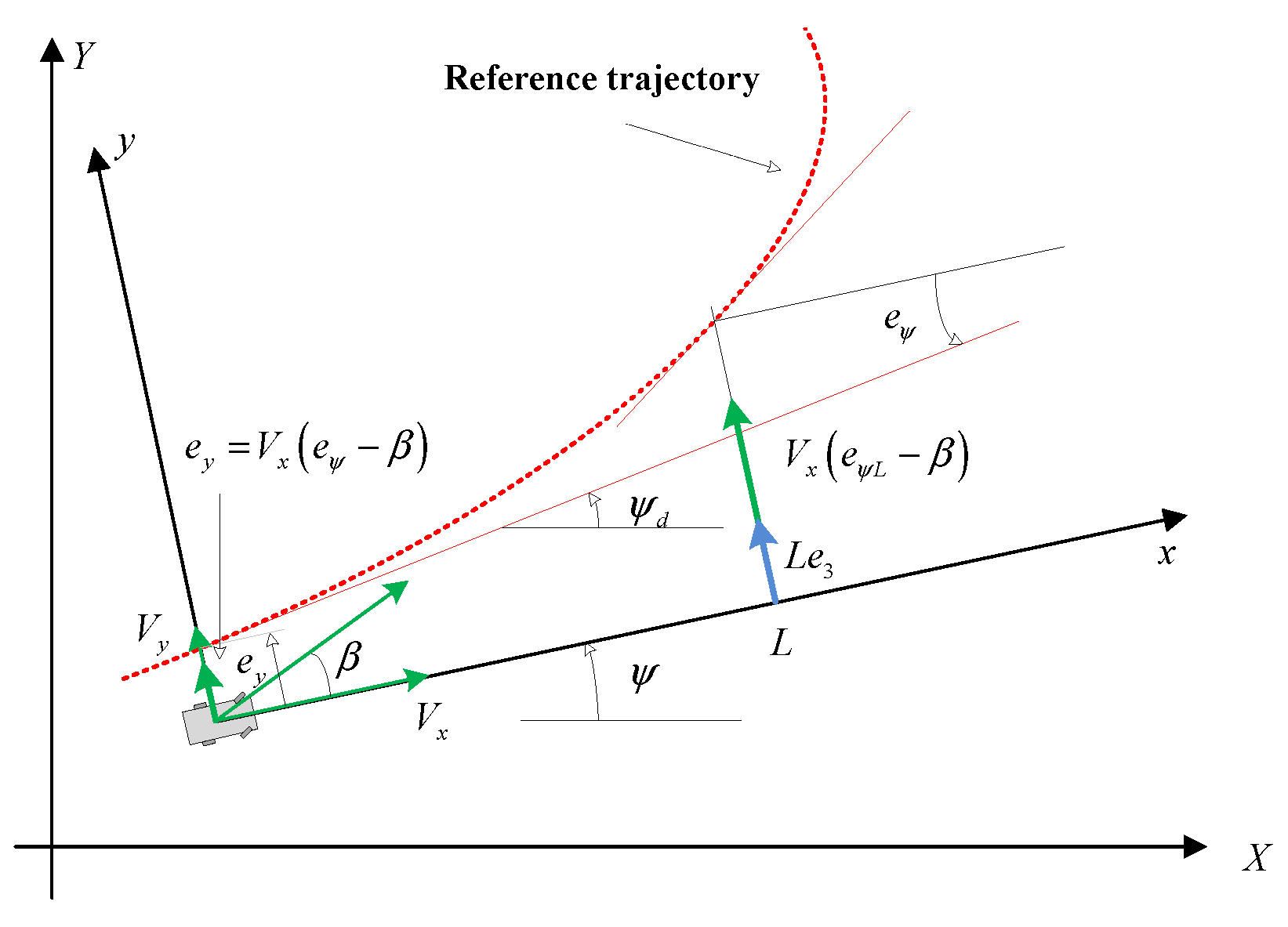
2. Vehicle Lateral Dynamics Modeling
3. Control Strategy for Collision Avoidance
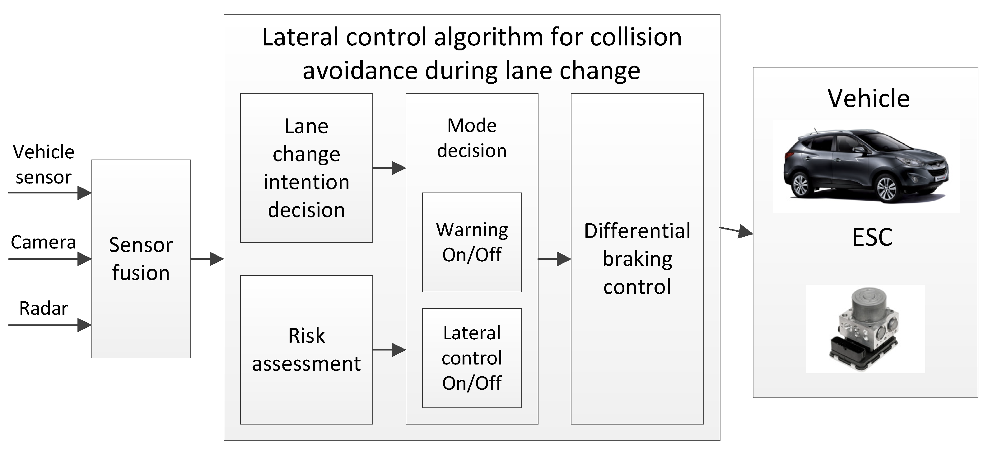
3.1. Structure of the Collision Avoidance System
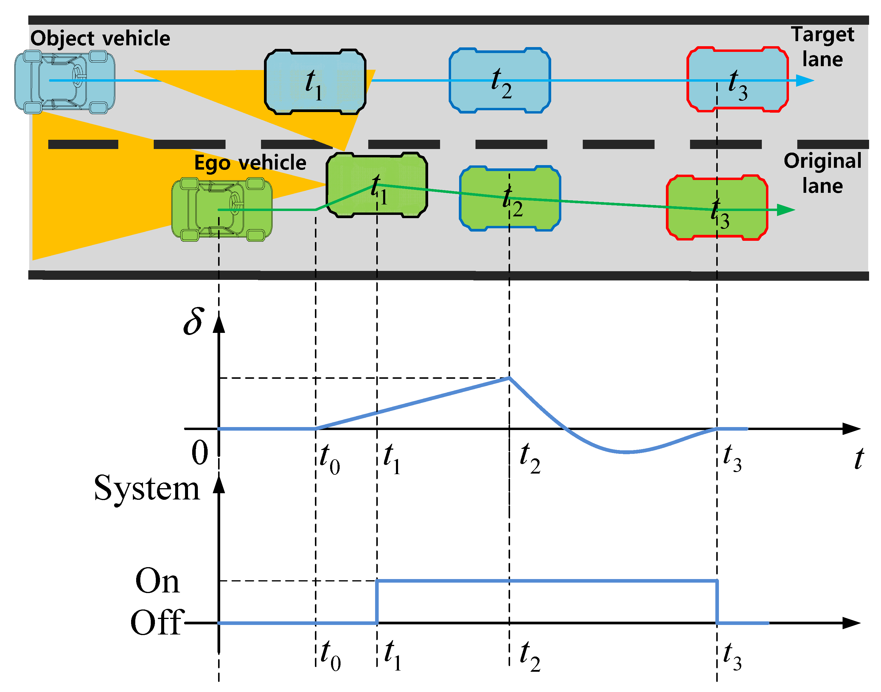
3.2. Strategy of Lateral Control for Collision Avoidance
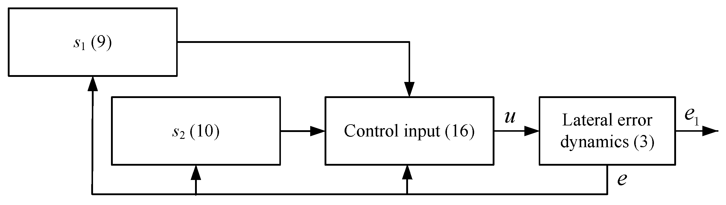
4. Differential Braking Control Algorithm Design for Lateral Control
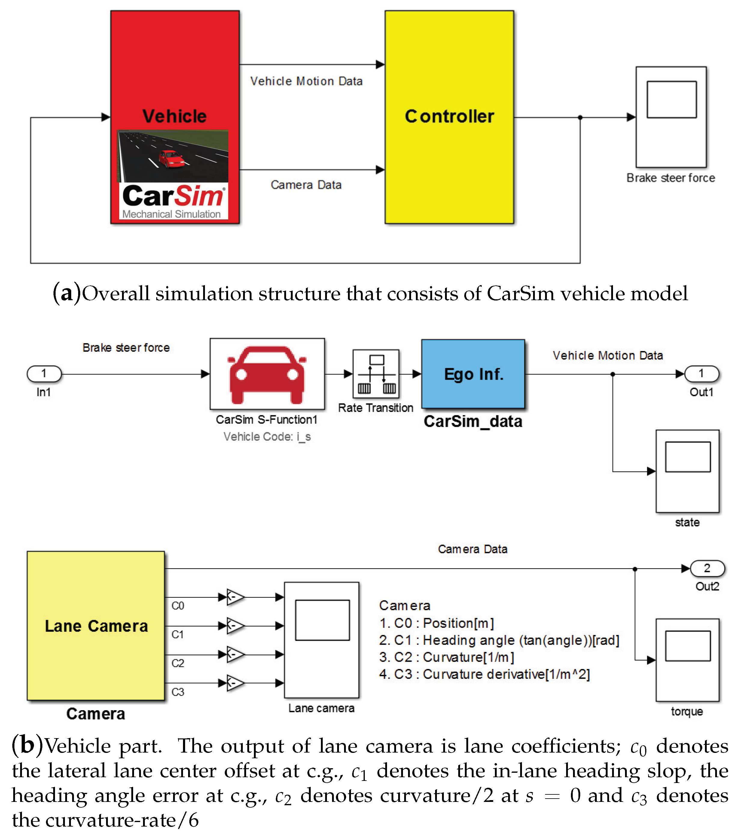
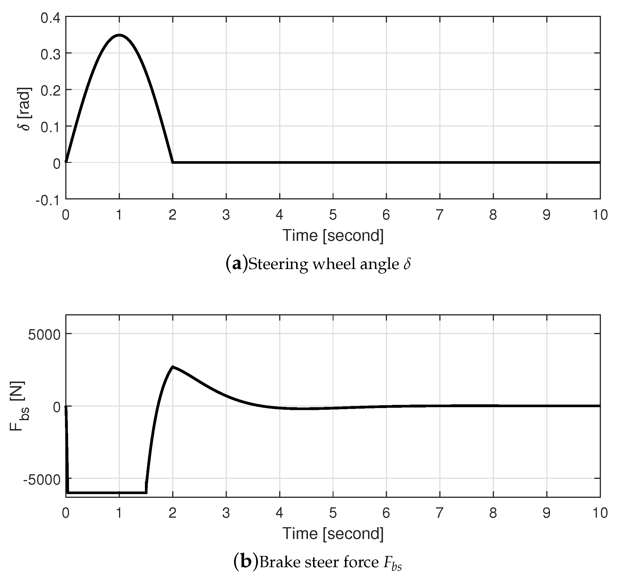
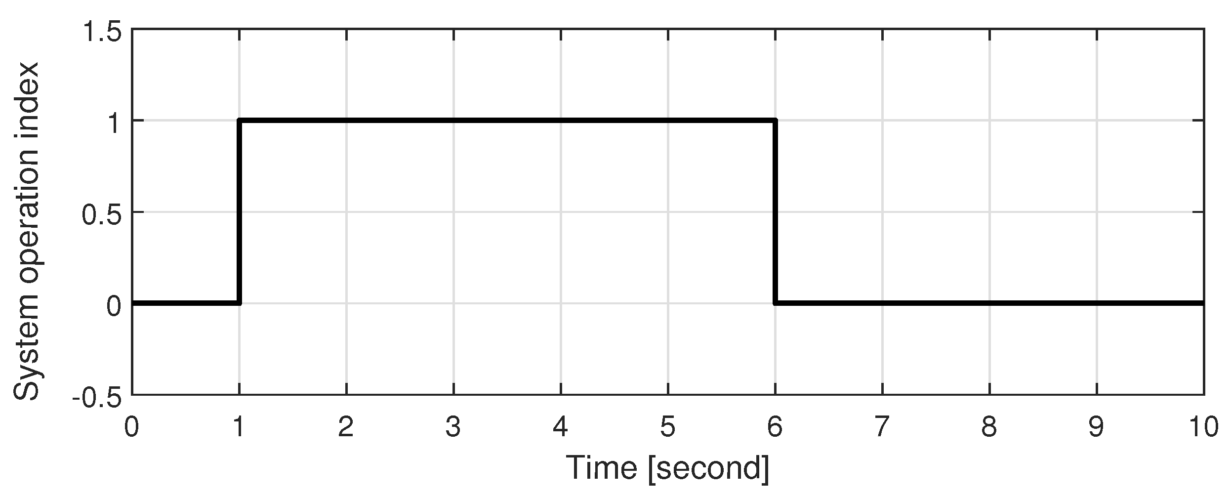
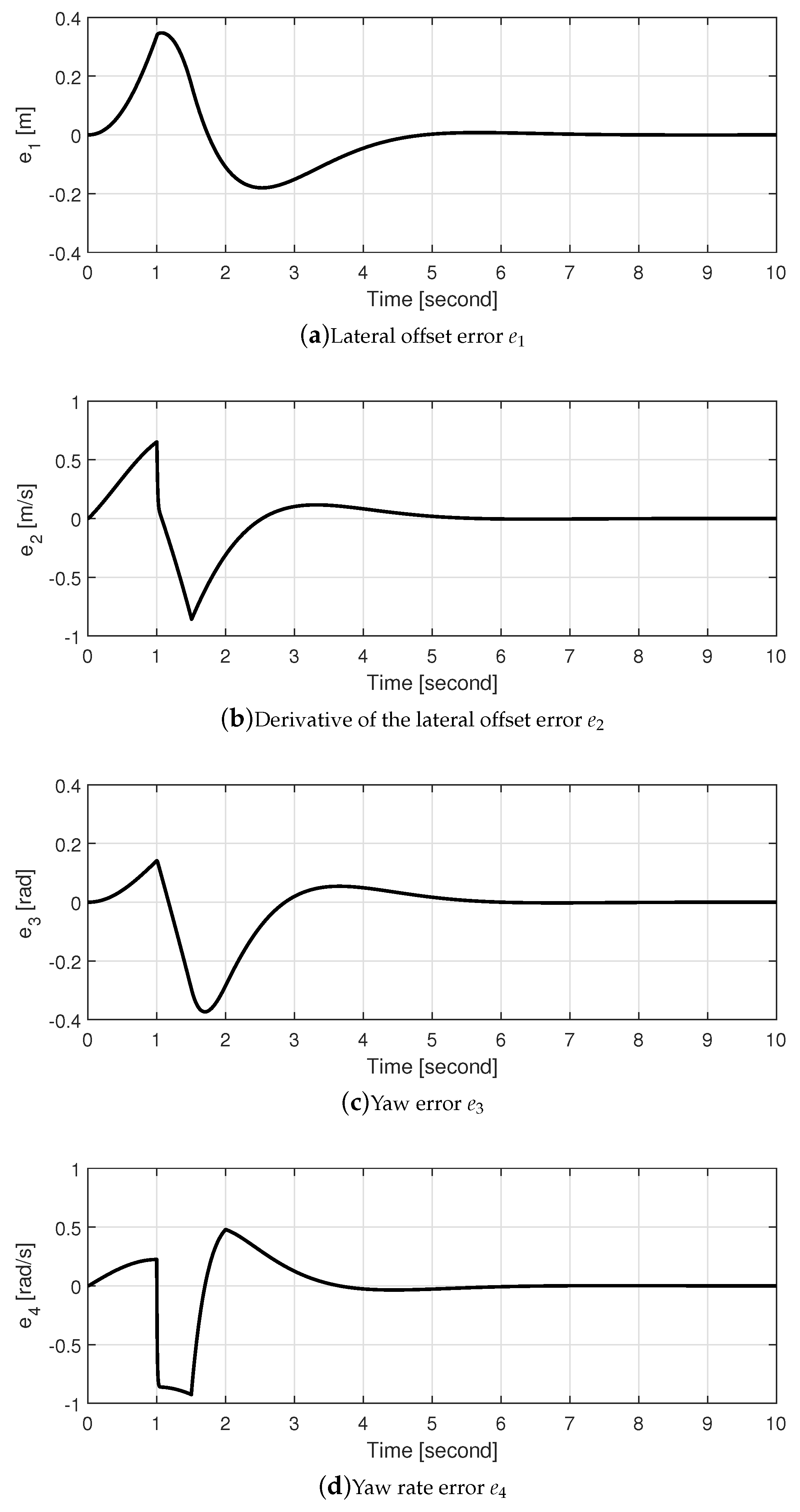
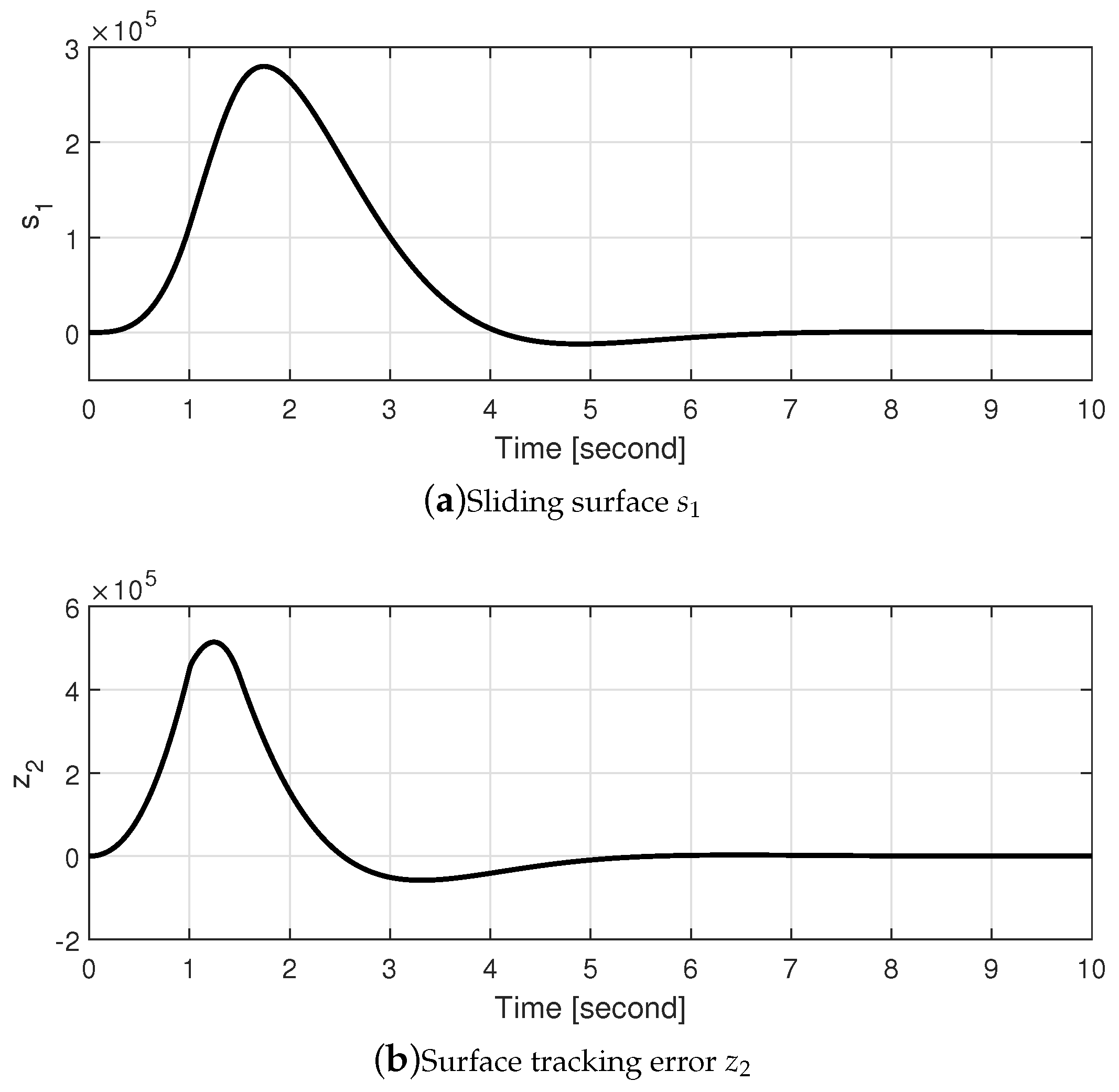
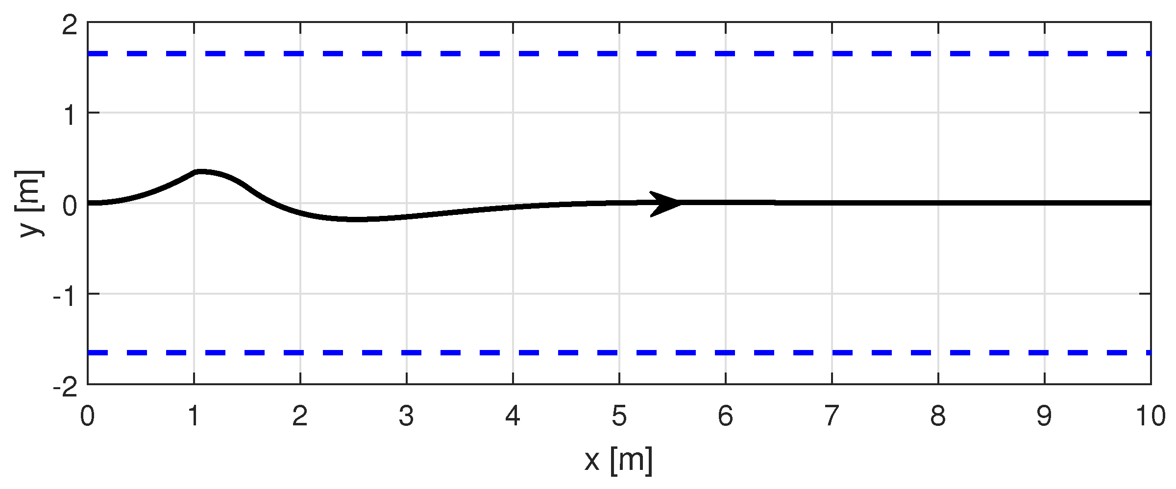
5. Simulation Results
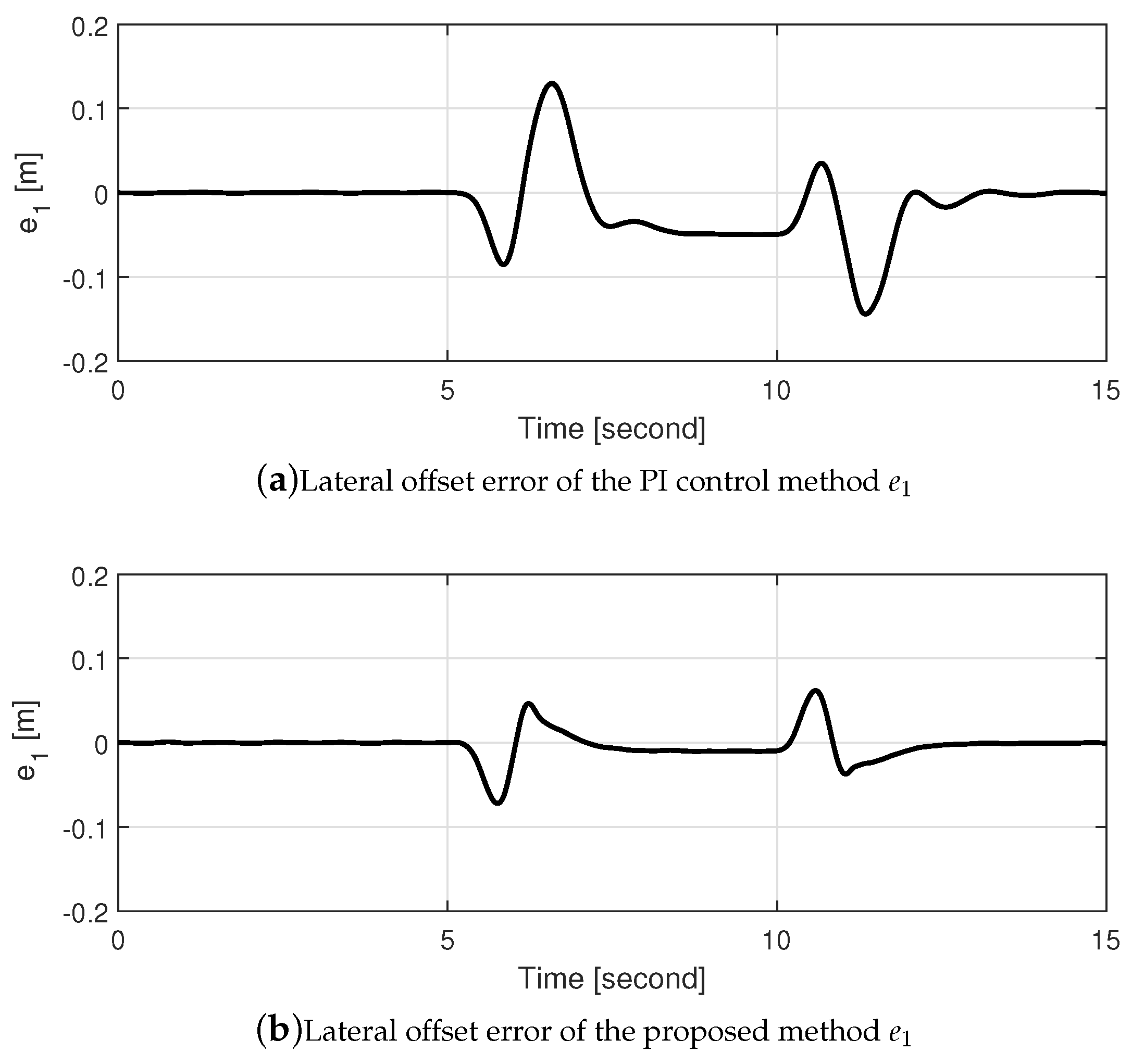
5.1. Straight Road
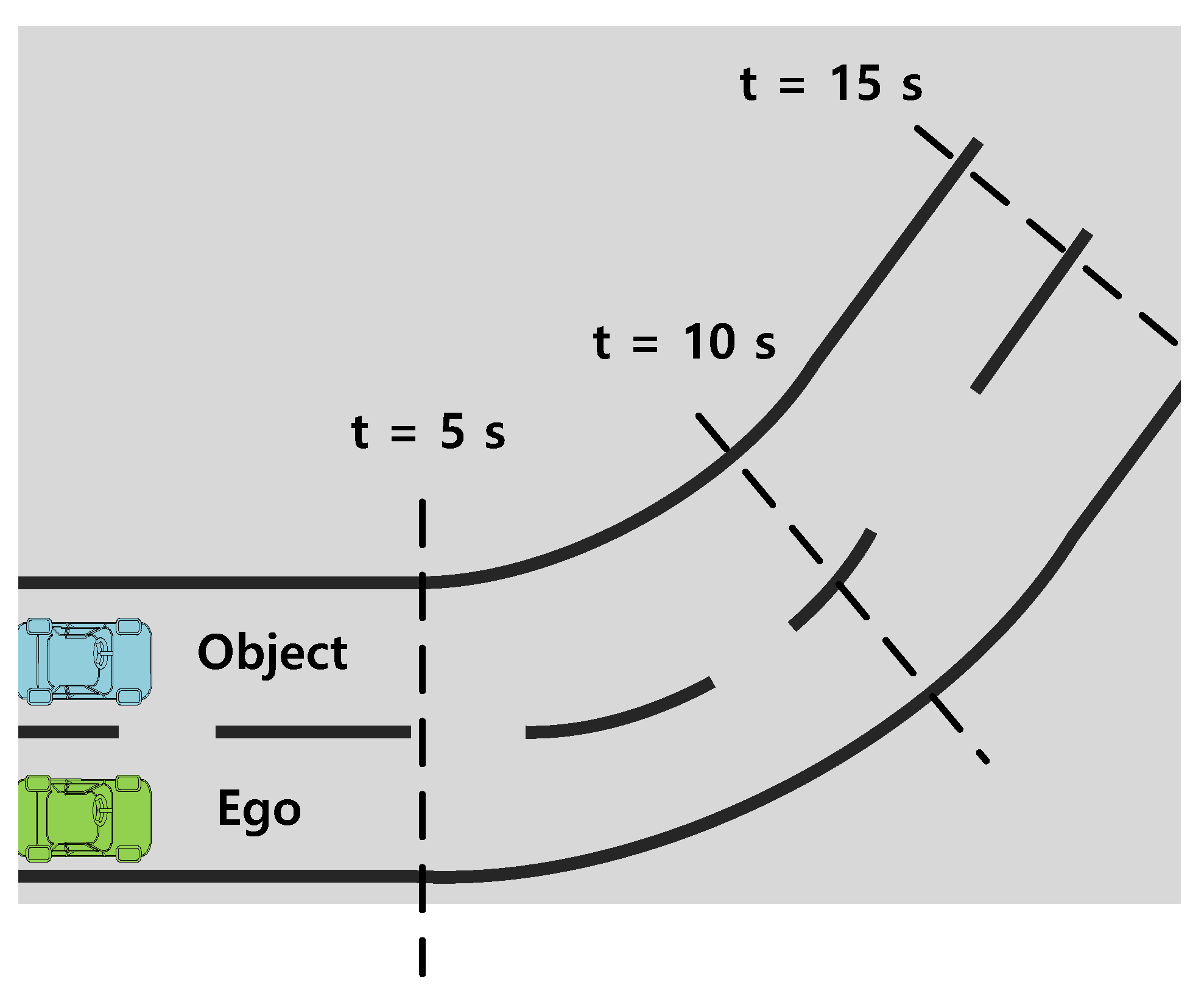
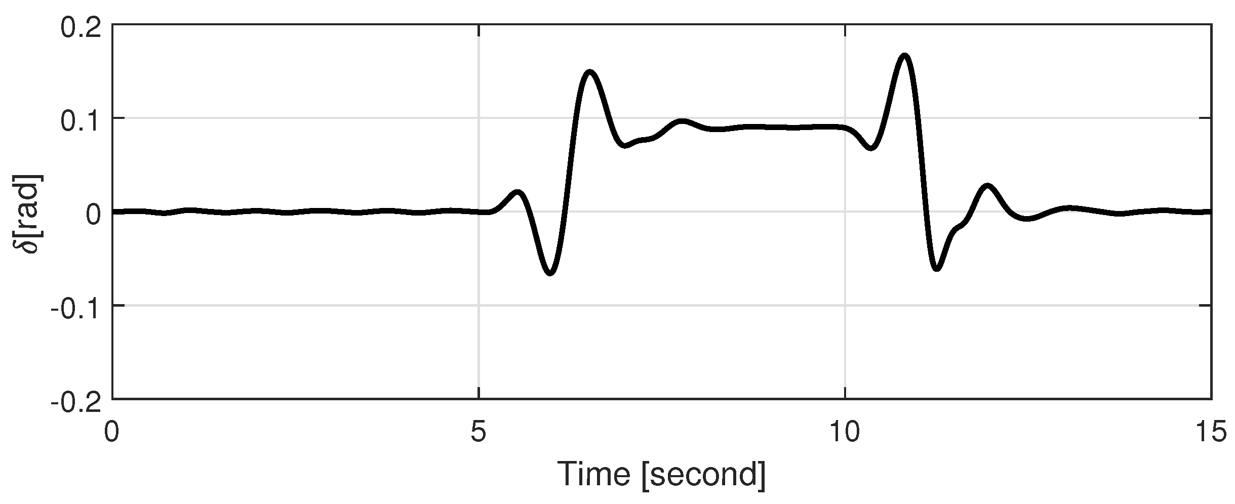
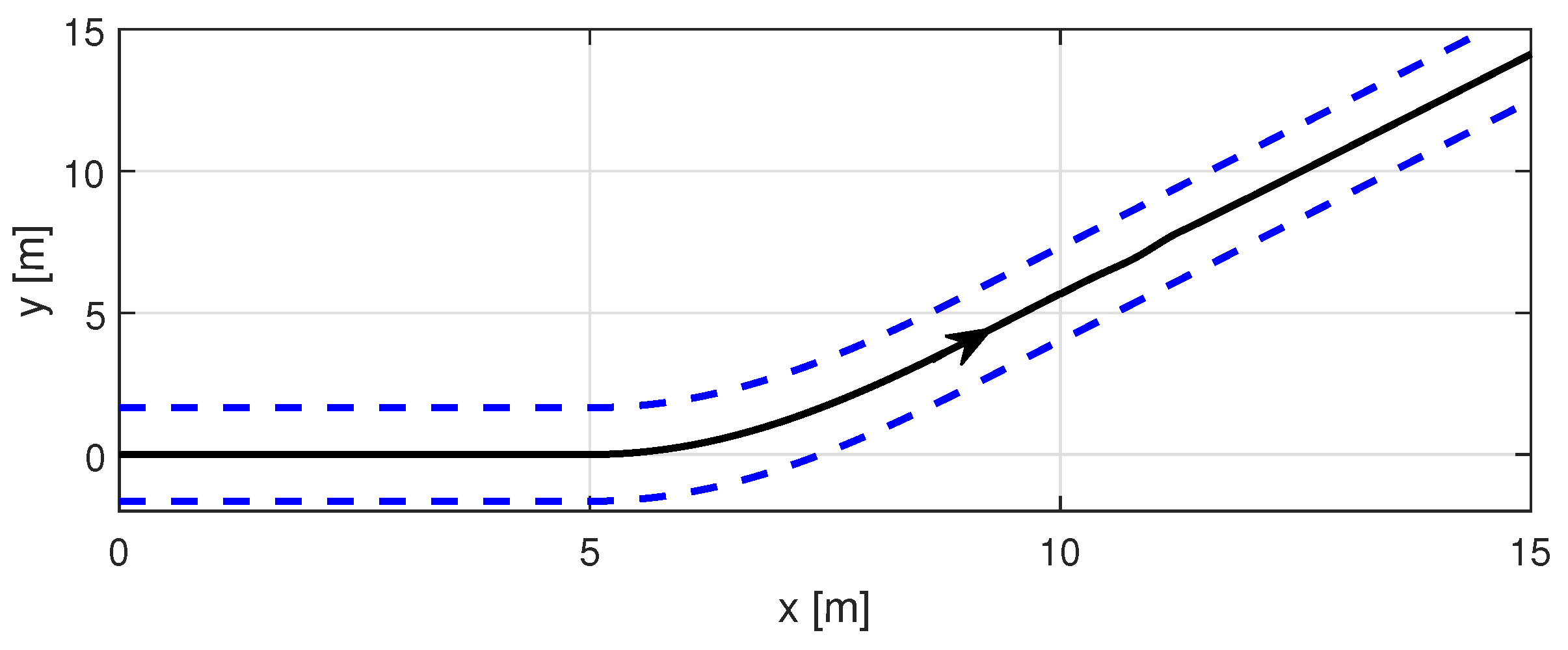
5.2. Curved Road
6. Conclusions
Author Contributions
Funding
Institutional Review Board Statement
Informed Consent Statement
Conflicts of Interest
References
- Zhang, Y.; Jing, L.; Sun, C.; Fang, J.; Feng, Y. Human factors related to major road traffic accidents in China. Traffic Inj. Prev. 2019, 20, 796–800. [Google Scholar] [CrossRef]
- Shaon, M.R.R.; Qin, X.; Chen, Z.; Zhang, J. Exploration of contributing factors related to driver errors on highway segments. Transp. Res. Rec. 2018, 2672, 22–34. [Google Scholar] [CrossRef]
- National Highway Traffic Safety Administration. Traffic Safety Facts 2005; Department of Transportation: Washington, DC, USA, 2006. [Google Scholar]
- Jula, H.; Kosmatopoulos, E.B.; Ioannou, P.A. Collision avoidance analysis for lane changing and merging. IEEE Trans. Veh. Technol. 2000, 46, 2295–2308. [Google Scholar] [CrossRef] [Green Version]
- Laugier, C.; Paromtchik, I.E.; Perrollaz, M.; Yong, M.; Yoder, J.-D.; Tay, C.; Mekhnacha, K.; Ne‘gre, A. Probabilistic analysis of dynamics scenes and collision risks assessment to improve driving safety. IEEE Trans. Intell. Trans. Syst. Mag. 2011, 3, 4–19. [Google Scholar] [CrossRef] [Green Version]
- Houe‘nou, A.; Bonnifait, P.; Cherfaoui, V. Risk assessment for collision avoidance systems. In Proceedings of the 17th International IEEE Conference on Intelligent Transportation Systems (ITSC), Qingdao, China, 8–11 October 2014; pp. 386–391. [Google Scholar]
- Kim, J.; Kum, D. Collision risk assessment algorithm via lane-based probabilistic motion prediction of surrounding vehicles. IEEE Trans. Intell. Transp. Syst. 2017, 19, 2965–2976. [Google Scholar] [CrossRef]
- Gao, H.; Zhu, J.; Zhang, T.; Xie, G.; Kan, Z.; Hao, Z.; Liu, K. Situational assessment for intelligent vehicles based on Stochastic model and Gaussian distributions in typical traffic scenarios. IEEE Trans. Syst. Man Cybern. Syst. 2021, 1–11. [Google Scholar] [CrossRef]
- Huang, M.; Gao, W.; Wang, Y.; Jiang, Z.P. Data-driven shared steering control of semi-autonomous vehicles. IEEE Trans. Hum. Mach. Syst. 2019, 49, 350–361. [Google Scholar] [CrossRef]
- Marcano, M.; Di´az, S.; Pérez, J.; Irigoyen, E. A review of shared control for automated vehicles: Theory and applications. IEEE Trans. Hum. Mach. Syst. 2020, 50, 475–491. [Google Scholar] [CrossRef]
- Chen, Y.; Zhang, X.; Wang, J. Robust vehicle driver assistance control for handover scenarios considering driving performances. IEEE Trans. Syst. Man Cybern. Syst. 2021, 51, 4160–4170. [Google Scholar] [CrossRef]
- Termous, H.; Shraim, H.; Talj, R.; Francis, C.; Charara, A. Coordinated control strategies for active steering, differential braking and active suspension for vehicle stability, handling and safety improvement. Veh. Syst. Dyn. 2019, 57, 1494–1529. [Google Scholar] [CrossRef]
- Hajiloo, R.; Abroshan, M.; Khajepour, A.; Kasaiezadeh, A.; Chen, S.K. Integrated steering and differential braking for emergency collision avoidance in autonomous vehicles. IEEE Trans. Intell. Transp. Syst. 2021, 22, 3167–3178. [Google Scholar] [CrossRef]
- Lin, Y.M.; Chen, B.C. Handling Enhancement of Autonomous Emergency Steering for Reduced Road Friction Using Steering and Differential Braking. Appl. Sci. 2021, 11, 4891. [Google Scholar] [CrossRef]
- Lee, J.; Choi, J.; Yi, K.; Shin, M.; Kob, B. Lane-keeping assistance control algorithm using differential braking to prevent unintended lane departures. Control Eng. Pr. 2014, 23, 1–13. [Google Scholar] [CrossRef]
- Pilutti, T.; Ulsoy, G.; Hrovat, D. Vehicle steering intervention through differential braking. J. Dyn. Sys. Meas. Control 1998, 120, 314–321. [Google Scholar] [CrossRef]
- Uematsu, K.; Gerdes, J.C. A comparison of several sliding surfaces for stability control. In Proceedings of the International Symposium on Advanced Vehicle Control, Hiroshima, Japan, 9–13 September 2002; pp. 601–608. [Google Scholar]
- Li, X.; Xu, N.; Guo, K.; Huang, Y. An adaptive SMC controller for EVs with four IWMs handling and stability enhancement based on a stability index. Veh. Syst. Dyn. 2021, 1–24. [Google Scholar] [CrossRef]
- Infinity, “Blind Spot Intervention” [Online]. Available online: Http://www.infinitiusa.com/now/technology/blind-spot-intervention-system.html (accessed on 15 May 2021).
- Kim, W.; Chen, X.; Lee, Y.; Chung, C.C.; Tomizuka, M. Discrete-time nonlinear damping backstepping control with observers for rejection of low and high frequency disturbances. Mech. Syst. Signal Process. 2018, 104, 436–448. [Google Scholar] [CrossRef]
- Park, J.-H.; Park, T.-S.; Kim, S.-H. Approximation-free output-feedback non-backstepping controller for uncertain SISO nonautonomous nonlinear pure-feedback systems. Mathematics 2019, 7, 456. [Google Scholar] [CrossRef] [Green Version]
- Kang, C.M.; Kim, W.; Baek, H. Cascade backstepping control with augmented observer for lateral control of vehicle. IEEE Access 2021, 9, 45367–45376. [Google Scholar] [CrossRef]
- Rajamani, R.; Tan, H.-S.; Law, B.K.; Zhang, W.-B. Demonstration of integrated longitudinal and lateral control for the operation of automated vehicles in platoons. IEEE Trans. Control Syst. Technol. 2000, 8, 695–708. [Google Scholar] [CrossRef]
- Rajamani, R. Vehicle Dynamics and Control, 2nd ed.; Springer: Berlin/Heidelberg, Germany, 2012. [Google Scholar]
- Ackermann, J. Robust car steering by yaw rate control. In Proceedings of the 29th IEEE Conference on Decision and Control, Honolulu, HI, USA, 5–7 December 1990; pp. 2033–2034. [Google Scholar]
- Son, Y.S.; Kim, W.; Lee, S.-H.; Chung, C.C. Asynchronous sensor fusion using multi-rate kalman filter. Trans Korean Inst. Elec. Eng. 2014, 63, 1551–1558. [Google Scholar] [CrossRef] [Green Version]
- Fayyad, J.; Jaradat, M.A.; Gruyer, D.; Najjaran, H. Deep learning sensor fusion for autonomous vehicle perception and localization: A review. Sensors 2020, 20, 4220. [Google Scholar] [CrossRef] [PubMed]
- Lin, B.-F.; Chan, Y.-M.; Fu, L.-C.; Hsiao, P.-Y.; Chuang, L.-A.; Huang, S.-S.; Lo, M.-F. Integrating appearance and edge features for sedan vehicle detection in the blind-spot area. IEEE Trans. Intell. Trans. Syst. 2012, 13, 737–747. [Google Scholar]
- Khalil, H. Nonlinear Systems, 3rd ed.; Prentice-Hall: Upper Saddle River, NJ, USA, 2002. [Google Scholar]
- Cheng, H.-Y.; Jeng, B.-S.; Tseng, P.-T.; Fan, K.-C. Lane detection with moving vehicles in the traffic scenes. IEEE Trans. Intell. Transp. Syst. 2006, 7, 571–582. [Google Scholar]


| Parameter | Value | Parameter | Value |
|---|---|---|---|
| 1,000,000 | 200 | ||
| 50 | 0 | ||
| 1 | 1 | ||
| 0.1 |
Publisher’s Note: MDPI stays neutral with regard to jurisdictional claims in published maps and institutional affiliations. |
© 2021 by the authors. Licensee MDPI, Basel, Switzerland. This article is an open access article distributed under the terms and conditions of the Creative Commons Attribution (CC BY) license (https://creativecommons.org/licenses/by/4.0/).
Share and Cite
Son, Y.S.; Kim, W. Nonlinear Differential Braking Control for Collision Avoidance During Lane Change. Mathematics 2021, 9, 1699. https://doi.org/10.3390/math9141699
Son YS, Kim W. Nonlinear Differential Braking Control for Collision Avoidance During Lane Change. Mathematics. 2021; 9(14):1699. https://doi.org/10.3390/math9141699
Chicago/Turabian StyleSon, Young Seop, and Wonhee Kim. 2021. "Nonlinear Differential Braking Control for Collision Avoidance During Lane Change" Mathematics 9, no. 14: 1699. https://doi.org/10.3390/math9141699