Article

Efficient Space–Time Reduced Order Model for Linear Dynamical Systems in Python Using Less than 120 Lines of Code

1
Mechanical Engineering, University of California, Berkeley, CA 94720, USA
2
Lawrence Livermore National Laboratory, Livermore, CA 94550, USA
3
Center for Applied Scientific Computing, Lawrence Livermore National Laboratory, Livermore, CA 94550, USA
*
Author to whom correspondence should be addressed.
These authors contributed equally to this work.
Mathematics 2021, 9(14), 1690; https://doi.org/10.3390/math9141690
Submission received: 17 May 2021 / Revised: 5 July 2021 / Accepted: 9 July 2021 / Published: 19 July 2021

Abstract

:
A classical reduced order model (ROM) for dynamical problems typically involves only the spatial reduction of a given problem. Recently, a novel space–time ROM for linear dynamical problems has been developed [Choi et al., Space–tume reduced order model for large-scale linear dynamical systems with application to Boltzmann transport problems, Journal of Computational Physics, 2020], which further reduces the problem size by introducing a temporal reduction in addition to a spatial reduction without much loss in accuracy. The authors show an order of a thousand speed-up with a relative error of less than 10 5 for a large-scale Boltzmann transport problem. In this work, we present for the first time the derivation of the space–time least-squares Petrov–Galerkin (LSPG) projection for linear dynamical systems and its corresponding block structures. Utilizing these block structures, we demonstrate the ease of construction of the space–time ROM method with two model problems: 2D diffusion and 2D convection diffusion, with and without a linear source term. For each problem, we demonstrate the entire process of generating the full order model (FOM) data, constructing the space–time ROM, and predicting the reduced-order solutions, all in less than 120 lines of Python code. We compare our LSPG method with the traditional Galerkin method and show that the space–time ROMs can achieve O ( 10 3 ) to O ( 10 4 ) relative errors for these problems. Depending on parameter–separability, online speed-ups may or may not be achieved. For the FOMs with parameter–separability, the space–time ROMs can achieve O ( 10 ) online speed-ups. Finally, we present an error analysis for the space–time LSPG projection and derive an error bound, which shows an improvement compared to traditional spatial Galerkin ROM methods.

1. Introduction

Many computational models for physical simulations are formulated as linear dynamical systems. Examples of linear dynamical systems include, but are not limited to, the Schrödinger equation that arises in quantum mechanics, the computational model for the signal propagation and interference in electric circuits, storm surge prediction models before an advancing hurricane, vibration analysis in large structures, thermal analysis in various media, neuro-transmission models in the nervous system, various computational models for micro-electro-mechanical systems, and various particle transport simulations. These linear dynamical systems can quickly become large scale and computationally expensive, which prevents fast generation of solutions. Thus, areas in design optimization, uncertainty quantification, and control where large parameter sweeps need to be done can become intractable, and this motivates the need for developing a Reduced Order Model (ROM) that can accelerate the solution process without loss in accuracy.
Many ROM approaches for linear dynamical systems have been developed, and they can be broadly categorized as data-driven or non data-driven approaches. We give a brief background of some of the methods here. For the non data-driven approaches, there are several methods, including: balanced truncation methods [1,2,3,4,5,6,7,8,9], moment-matching methods [10,11,12,13,14], and Proper Generalized Decomposition (PGD) [15] and its extensions [16,17,18,19,20,21,22,23,24,25]. The balanced truncation method is by far the most popular method, but it requires the solution of two Lyapunov equations to construct bases, which is a computationally expensive task in large-scale problems using dense solvers. However, the fast and memory-efficient low rank solvers presented in [26,27] can be applied to the large-scale Lyapunov equations. On the other hand, this expensive task can be bypassed by various data-driven empirical and non-intrusive approaches [3,28,29,30,31]. Moment matching methods were originally developed as non data-driven, although later studies developed ideas to benefit from the data. They provide a computationally efficient framework using Krylov subspace techniques in an iterative fashion where only matrix–vector multiplications are required. The optimal H 2 tangential interpolation for nonparametric systems [11] is also available. Proper Generalized Decomposition was first developed as a numerical method for solving boundary value problems. It utilizes techniques to separate space and time for an efficient solution procedure and is considered a model reduction technique. For the detailed description of PGD, we refer to a short review paper [32]. Many data driven ROM approaches have been developed as well. When datasets are available either from experiments or high-fidelity simulations, these datasets can contain rich information about the system of interest and utilizing this in the construction of a ROM can produce an optimal basis. Although there are some data-driven moment matching works available [33,34], two popular methods are Dynamic Mode Decomposition (DMD) and Proper Orthogonal decomposition (POD). DMD generates reduced modes that embed an intrinsic temporal behavior and was first developed by Peter Schmid [35]. The method has been actively developed and extended to many applications [36,37,38,39,40,41,42,43]. For a more detailed description about DMD, we refer to this preprint [44] and book [45]. POD utilizes the method of snapshots to obtain an optimal basis of a system and typically applies only to spatial projections [46,47,48,49,50,51,52,53,54,55,56,57,58,59,60,61].
Although the data-driven ROMs have brought many benefits, such as speed-ups and accuracy, they have been mainly the reduction of the complexity on spatial domains. However, reducing the temporal domain complexity brings even more speed-ups for time dependent problems. Therefore, we focus on building a space–time ROM, where both spatial and temporal projections are applied to achieve an optimal reduction. Several space–time ROMs have been developed, including, but not limited to, the ones derived from the corresponding space–time full order models [62,63,64,65], the spectral POD and resolvent modes-based ones [66,67,68], and the ones that take advantage of the right singular vectors [69,70,71]. In particular, a space–time ROM for large-scale linear dynamical systems has been recently introduced [72]. The authors show a speed-up of greater than 8000 with good accuracy for a large-scale transport problem. However, the space–time ROM in [72] was limited to Galerkin projection, which can cause stability issues [22,73,74] for nonlinear problems. It is well-studied that the LSPG ROM formulation [75] brings various benefits, such as better stability, over Galerkin projection with some known issues, such as structure preservation [76]. Furthermore, it is not clear if the space–time least-squares Petrov–Galerkin (LSPG) brings any advantage over the space–time Galerkin approach for a linear dynamical system. The current manuscript addresses this aspect.
In this work, we present several contributions on the space–time ROM development for linear dynamical systems:
  • We derive the block structures of least-squares Petrov–Galerkin (LSPG) space–time ROM operators for linear dynamical systems for the first time and compare them with the Galerkin space–time ROM operators.
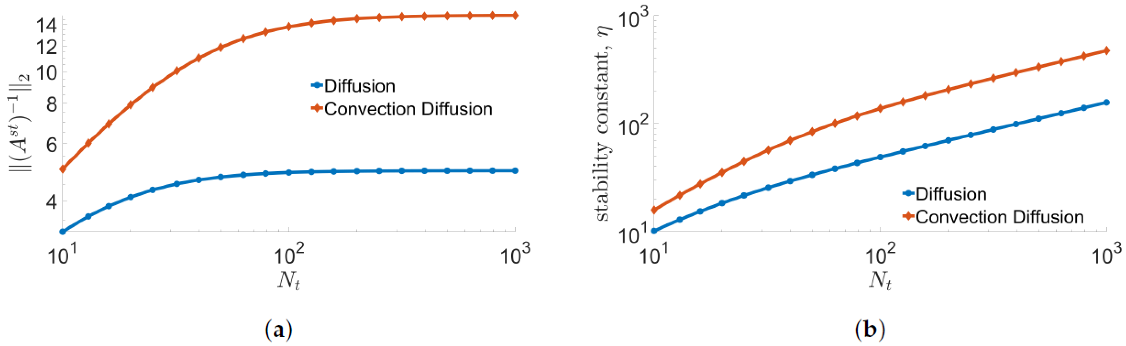
  • We present an error analysis for LSPG space–time ROMs for the first time and demonstrate the growth rate of the stability constant with the actual space–time operators used in our numerical results.
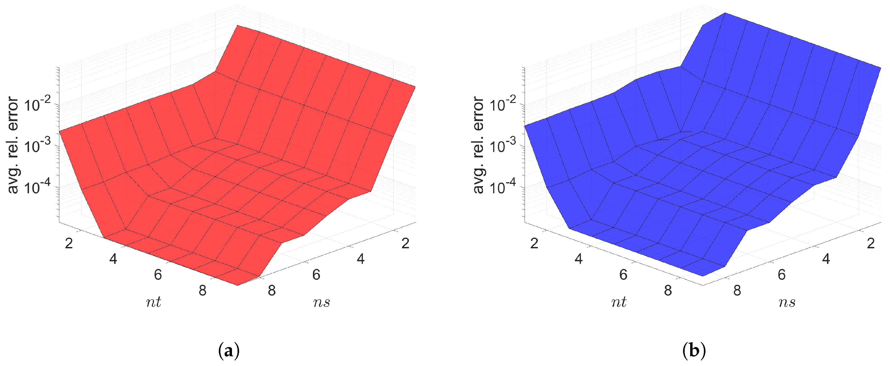
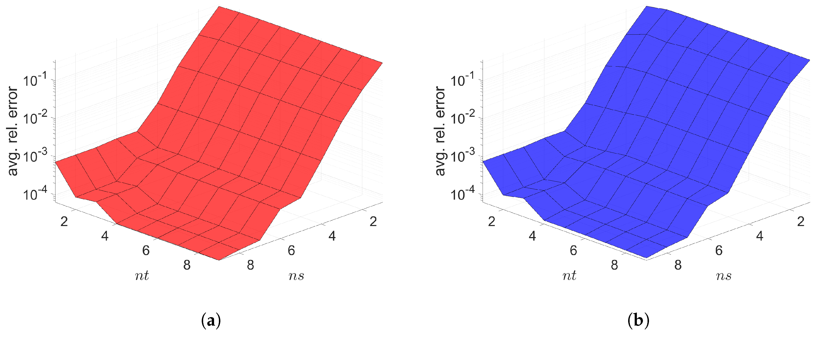
  • We compare the performance between space–time Galerkin and space–time LSPG reduced order models on several linear dynamical systems.
  • For each numerical problem, we cover the entire space–time ROM process in less than 120 lines of Python code, which includes sweeping a wide parameter space and generating data from the full order model, constructing the space–time ROM, and generating the ROM prediction in the online phase.
We note that the first two bullet points above are minor but useful contributions by making the block structure and error analysis readily available. Additionally, we hope that, by providing full access to the Python source codes, researchers can easily apply space–time ROMs to their linear dynamical problem of interest. Furthermore, we have curated the source codes to be simple and short so that it may be easily extended in various multi-query problem settings, such as design optimization [77,78,79,80,81,82,83], uncertainty quantification [84,85,86], and optimal control problems [87,88,89].
The paper is organized in the following way: Section 2 describes a parametric linear dynamical systems and space–time formulation. Section 3 introduces linear subspace solution representation in Section 3.1 and space–time ROM formulation using Galerkin projection in Section 3.2 and LSPG projection in Section 3.3. Then, both space–time ROMs are compared in Section 3.4. Section 4 describes how to generate space–time basis. We investigate block structures of space–time ROM basis in Section 5.1. We introduce the block structures of Galerkin space–time ROM operators derived in [72] in Section 5.2. In Section 5.3, we derive LSPG space–time ROM operators in terms of the blocks. Then, we compared Galerkin and LSPG block structures in Section 5.4. We show computational complexity of forming the space–time ROM operators in Section 5.5. The error analysis is presented in Section 6. We demonstrate the performance of both Galerkin and LSPG space–time ROMs in two numerical experiments in Section 7. Finally, the paper is concluded with summary and future works in Section 8. Appendix A presents six Python codes with less than 120 lines that are used to generate our numerical results.

2. Linear Dynamical Systems

We consider the parameterized linear dynamical system shown in Equation (1):
u ( t ; μ ) t = A ( μ ) u ( t ; μ ) + B ( μ ) f ( t ; μ ) , u ( 0 ; μ ) = u 0 ( μ ) ,
where μ Ω μ R N μ denotes a parameter vector, u : [ 0 , T ] × R N μ R N s denotes a time dependent state variable function, u 0 : R N μ R N s denotes an initial state, and f : [ 0 , T ] × R N μ R N i denotes a time dependent input variable function. The operators A : R N μ R N s × N s and B : R N μ R N s × N i are real valued matrices that are independent of state variables.
Although any time integrator can be used, for the demonstration purpose, we choose to apply a backward Euler time integration scheme shown in Equation (2):
I N s Δ t ( k ) A ( μ ) u ( k ) = u ( k 1 ) + Δ t ( k ) B ( μ ) f ( k ) ( μ ) ,
where I N s R N s × N s is the identity matrix, Δ t ( k ) is the kth time step size with T = k = 1 N t Δ t ( k ) and t ( k ) = j = 1 k Δ t ( j ) , and u ( k ) ( μ ) : = u ( t ( k ) ; μ ) and f ( k ) ( μ ) : = f ( t ( k ) ; μ ) are the state and input vectors at the kth time step where k N ( N t ) . The Full Order Model (FOM) solves Equation (2) for every time step, where its spatial dimension is N s and the temporal dimension is N t . Each time step of the FOM can be written out and put in another matrix system shown in Equation (3). This is known as the space–time formulation.
A st ( μ ) u st ( μ ) = f st ( μ ) + u 0 st ( μ ) ,
where
A st ( μ ) = I N s Δ t ( 1 ) A ( μ ) I N s I N s Δ t ( 2 ) A ( μ ) I N s I N s Δ t ( N t ) A ( μ ) ,
u st ( μ ) = u ( 1 ) ( μ ) u ( 2 ) ( μ ) u ( N t ) ( μ ) ,
f st ( μ ) = Δ t ( 1 ) B ( μ ) f ( 1 ) ( μ ) Δ t ( 2 ) B ( μ ) f ( 2 ) ( μ ) Δ t ( N t ) B ( μ ) f ( N t ) ( μ ) ,
u 0 st ( μ ) = u 0 ( μ ) 0 0 .
The space–time system matrix A st has dimensions R N μ R N s N t × N s N t , the space–time state vector u st has dimensions R N μ R N s N t , the space–time input vector f st has dimensions R N μ R N s N t , and the space–time initial vector u 0 st has dimensions R N μ R N s N t . Although it seems that the solution can be found in a single solve, in practice, there is no computational saving gained from doing so since the block structure of the space–time system will solve the system in a time-marching fashion anyways. However, we formulate the problem in this way since our reduced order model (ROM) formulation can reduce and solve the space–time system efficiently. In the following sections, we describe the parametric Galerkin and LSPG ROM formulations.

3. Space–Time Reduced Order Models

We investigate two projection-based space–time ROM formulations: the Galerkin and LSPG formulations.

3.1. Linear Subspace Solution Representation

Both the Galerkin and LSPG methods reduce the number of space–time degrees of freedom by approximating the space–time state variables as a smaller linear combination of space–time basis vectors:
u st ( μ ) u ˜ st ( μ ) Φ st u ^ st ( μ ) ,
where u ^ st ( μ ) : R N μ R n s n t with n s N s and n t N t . The space–time basis, Φ st R N s N t × n s n t is defined as
Φ st ϕ 1 st ϕ i + n s ( j 1 ) st ϕ n s n t st ,
where i N ( n s ) , j N ( n t ) . Substituting Equation (8) into the space–time formulation in Equation (3) gives an over-determined system of equations:
A st ( μ ) Φ st u ^ st ( μ ) = f st ( μ ) + u 0 st ( μ )
This over-determined system of equations can be closed by either the Galerkin or LSPG projections.

3.2. Galerkin Projection

In the Galerkin formulation, Equation (10) is closed by the Galerkin projection, where both sides of the equation of multiplied by Φ st T . Thus, we solve following reduced system for the unknown generalized coordinates, u ^ st :
Φ st T A s t ( μ ) Φ st u ^ st ( μ ) = Φ st T f st ( μ ) + Φ st T u 0 st ( μ ) .
For notational simplicity, let us define the reduced space–time system matrix as A ^ s t , g ( μ ) : = Φ st T A s t ( μ ) Φ st , reduced space–time input vector as f ^ s t , g ( μ ) : = Φ st T f st ( μ ) , and reduced space–time initial state vector as u ^ 0 s t , g ( μ ) : = Φ st T u 0 st ( μ ) .

3.3. Least-Squares Petrov–Galerkin (LSPG) Projection

In the LSPG formulation, we first define the space–time residual as
r ˜ st ( u ^ st ; μ ) : = f st ( μ ) + u 0 st ( μ ) A st ( μ ) Φ st u ^ st
where r ˜ st : R n s n t × R N μ R N s N t . Note Equation (12) is an over-determined system. To close the system and solve for the unknown generalized coordinates, u ^ st , the LSPG method takes the squared norm of the residual vector function and minimize it:
u ^ st = argmin v ^ R n s n t 1 2 r ˜ st ( v ^ ; μ ) 2 2 .
The solution to Equation (13) satisfies
( A s t ( μ ) Φ st ) T r ˜ st ( u ^ st ; μ ) = 0
leading to
Φ st T A s t ( μ ) T A s t ( μ ) Φ st u ^ st ( μ ) = Φ st T A s t ( μ ) T f st ( μ ) + Φ st T A s t ( μ ) T u 0 st ( μ ) .
For notational simplicity, let us define the reduced space–time system matrix as
A ^ s t , p g ( μ ) : = Φ st T A s t ( μ ) T A s t ( μ ) Φ st ,
reduced space–time input vector as f ^ s t , p g ( μ ) : = Φ st T A s t ( μ ) T f st ( μ ) , and reduced space–time initial state vector as u ^ 0 s t , p g ( μ ) : = Φ st T A s t ( μ ) T u 0 st ( μ ) .

3.4. Comparison of Galerkin and LSPG Projections

The reduced space–time system matrices, reduced space–time input vectors, and reduced space–time initial state vectors for Galerkin and LSPG projections are presented in Table 1.

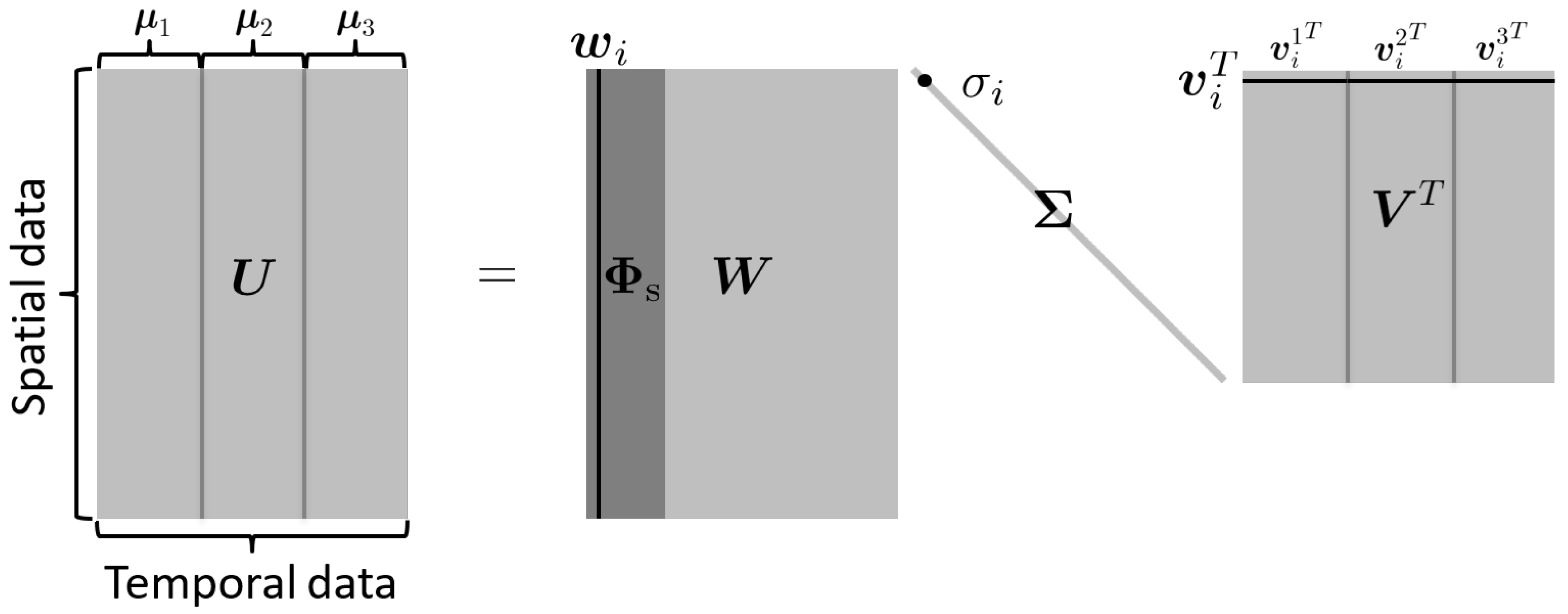
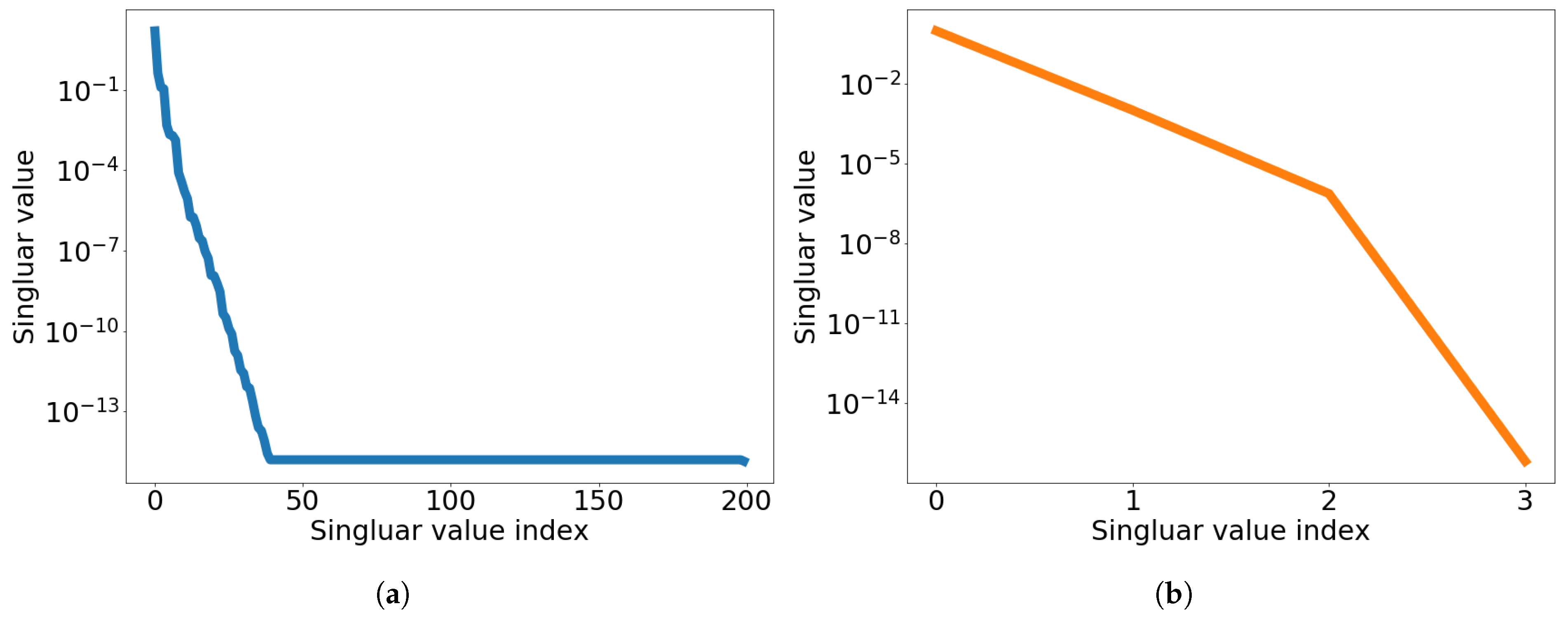
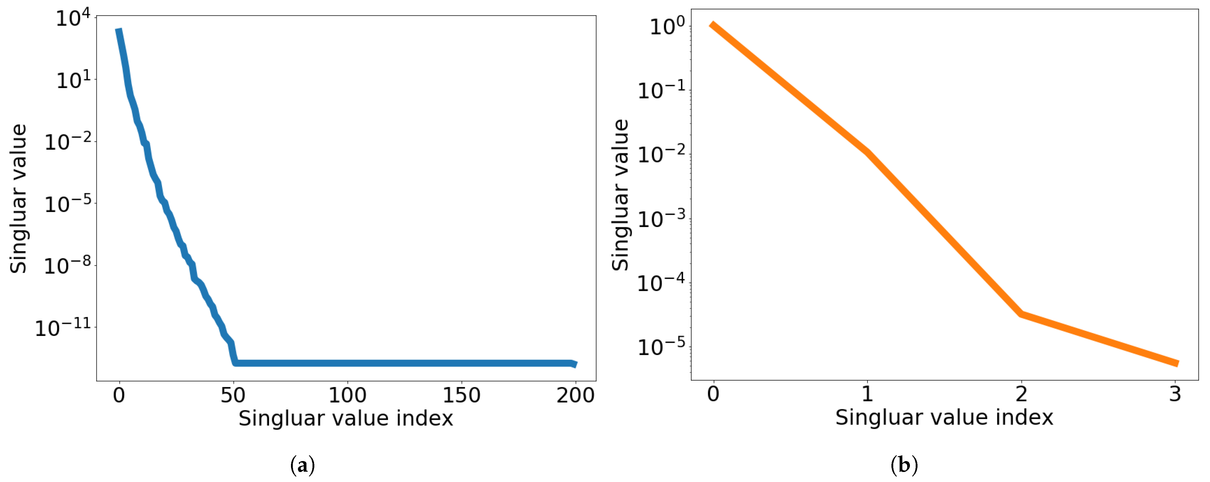
4. Space-Time Basis Generation

In this section, we repeat Section 4.1 in [72] to be self-contained.
A data set for space–time basis generation is chosen by the method of snapshots introduced by Sirovich [90]. This data set is called a snapshot matrix. By solving full order model problems at each of parameters in a parameter set { μ 1 , , μ n μ } , we obtain a full order model solution matrix U p at a certain parameter μ p , p N ( n μ ) , i.e.,
U p u ( 1 ) ( μ p ) u ( k ) ( μ p ) u ( N t ) ( μ p ) ,
where u ( k ) ( · ) R N s is a solution at a time step k N ( N t ) . Concatenating all the solution matrices for the every parameter yields the snapshot matrix, which is given by
U U 1 U n μ R N s × n μ N t .
To generate the spatial basis Φ s , Proper Orthogonal Decomposition (POD) is used [49]. The POD procedure seeks the reduced dimensional subspace that optimally represents the solution snapshot, U . The spatial POD basis Φ s is obtained by solving the following minimization problem:
Φ s = argmin Φ R N s × n s U Φ Φ T U F 2 s . t . Φ T Φ = I n s ,
where · F denotes the Frobenius norm and I n s R n s × n s is the identity matrix with n s < n μ N t . Then, the solution to the minimization problem is obtained by choosing the leading n s columns of the left singular matrix of Singular Value Decomposition (SVD) of the snapshot matrix U :
U = W Σ V T
where W R N s × and V R n μ N t × are orthogonal matrices and Σ R × is a diagonal matrix with singular values on its diagonal with min ( N s , n μ N t ) .
Equation (19) can be written in the summation form
U = i = 1 σ i w i v i T ,
where σ i R is the ith singular value, w i and v i are the ith left and right singular vectors, respectively. Here, n μ different temporal behavior of w i are represented by v i , e.g., v i 1 , v i 2 , and v i 3 describe three different temporal behavior of a certain basis vector w i in Figure 1. Now, let us set Y i = v i 1 v i n μ to be a temporal snapshot matrix associated with the ith spatial basis vector w i , where v i k [ v i ( 1 + ( k 1 ) N t ) , v i ( 2 + ( k 1 ) N t ) , , v i ( k N t ) ] T R N t for k N ( n μ ) , where v i ( j ) , j N ( n μ N t ) is the jth component of the vector v i . Then, applying SVD on Y i gives us
Y i = Λ i Σ i Ψ i T .
Leading n t vectors of the left singular matrix Λ i become the temporal basis Φ t i which describes a temporal behavior of the ith column of spatial basis Φ s . Finally, we construct a space–time basis vector ϕ i + n s ( j 1 ) st R N s N t given in Equation (9) as
ϕ i + n s ( j 1 ) st = ϕ i j t ϕ i s ,
where ⊗ denotes Kronecker product, ϕ i s R N s is the ith column of the spatial basis Φ s and ϕ i j t R N t is the jth column of the temporal basis Φ t i .

5. Space-Time Reduced Order Models in Block Structure

We avoid building the space–time basis vector defined in Equation (22) because it requires a lot of memory for storage. Instead, we can exploit the block structure of the matrices to save computational cost and storage of the matrices in memory. Section 5.2 introduces such block structures for the space–time Galerkin projection, while Section 5.3 shows block structures for the space–time LSPG projection. First of all, we introduce common block structures that appear both in the Galerkin and LSPG projections.

5.1. Block Structures of Space–Time Basis

Following [72]’s notation, we define the block structure of the space–time basis to be:
Φ s t = Φ s D 1 1 Φ s D 1 n t Φ s D k j Φ s D N t 1 Φ s D N t n t R N s N t × n s n t
where the kth time step of the temporal basis matrix is a diagonal matrix defined as
D k j = ϕ 1 j , k t 0 0 0 0 0 ϕ i j , k t 0 0 0 0 ϕ n s j , k t R n s × n s
where ϕ i j , k t R is the kth element of ϕ i j t R N t .

5.2. Block Structures of Galerkin Projection

As shown in Table 1, the reduced space–time Galerkin system matrix, A ^ s t , g ( μ ) is:
A ^ s t , g ( μ ) = Φ st T A s t ( μ ) Φ st
Now, we define the block structure of this matrix as:
A ^ s t , g ( μ ) = A ^ ( 1 , 1 ) s t , g ( μ ) A ^ ( 1 , n t ) s t , g ( μ ) A ^ ( j , j ) s t , g ( μ ) A ^ ( n t , 1 ) s t , g ( μ ) A ^ ( n t , n t ) s t , g ( μ )
so that we can exploit the block structure of these matrices such that we do not need to form the entire matrix. By inserting Equations (4) and (23) to Equation (25), we derive that the ( j , j ) th block matrix A ^ ( j , j ) s t , g ( μ ) R n s × n s is:
A ^ ( j , j ) s t , g ( μ ) = k = 1 N t D k j D k j Δ t ( k ) D k j Φ s T A ( μ ) Φ s D k j k = 1 N t 1 D k + 1 j D k j .
The reduced space–time Galerkin input vector f ^ s t , g ( μ ) R n s n t is
f ^ s t , g ( μ ) = Φ st T f st ( μ ) .
Again, utilizing the block structure of matrices, we compute the jth block vector f ^ s t , g ( μ ) ( j ) R n t to be:
f ^ s t , g ( μ ) ( j ) = k = 1 N t Δ t ( k ) D k j Φ s T B ( μ ) f ( k ) ( μ ) .
Finally, the space–time Galerkin initial vector, u ^ 0 s t , g ( μ ) R n s n t , can be computed as:
u ^ 0 s t , g ( μ ) = Φ st T u 0 st ( μ )
where the jth block vector, u ^ 0 s t , g ( μ ) ( j ) R n s , is:
u ^ 0 s t , g ( μ ) ( j ) = D 1 j Φ s T u 0 ( μ ) .

5.3. Block Structures of LSPG Projection

In Section 3.3, the reduced space–time LSPG system matrix, A ^ s t , p g ( μ ) is defined as
A ^ s t , p g ( μ ) = Φ s t T A s t ( μ ) T A s t ( μ ) Φ s t .
Then, the block structure of this matrix can be defined as
A ^ s t , p g ( μ ) = A ^ ( 1 , 1 ) s t , p g ( μ ) A ^ ( 1 , n t ) s t , p g ( μ ) A ^ ( j , j ) s t , p g ( μ ) A ^ ( n t , 1 ) s t , p g ( μ ) A ^ ( n t , n t ) s t , p g ( μ ) ,
where the size of each block matrix is n s × n s . Instead of forming the A ^ s t , p g ( μ ) directly from Equation (32), each block matrix A ^ ( j , j ) s t , p g ( μ ) R n s × n s is computed and put into its location. Inserting Equations (4) and (23) to Equation (32) gives us A ^ s t , p g ( μ ) and the ( j , j ) th block of this matrix is derived as
A ^ ( j , j ) s t , p g ( μ ) = k = 1 N t D k j Φ s T I N s Δ t ( k ) A ( μ ) T I N s Δ t ( k ) A ( μ ) Φ s D k j + k = 1 N t 1 [ D k j D k j D k j Φ s T I N s Δ t ( k + 1 ) A ( μ ) Φ s D k + 1 j D k + 1 j Φ s T I N s Δ t ( k + 1 ) A ( μ ) T Φ s D k j ] .
The reduced space–time LSPG input vector f ^ s t , p g ( μ ) R n s n t is given by
f ^ s t , p g ( μ ) = Φ s t T A s t ( μ ) T f st ( μ ) ,
where the jth block vector f ^ s t , p g ( μ ) ( j ) R n t is computed as
f ^ s t , p g ( μ ) ( j ) = k = 1 N t D k j Φ s T I N s Δ t ( k ) A ( μ ) T Δ t ( k ) B ( μ ) f ( k ) ( μ ) k = 1 N t 1 D k j Φ s T Δ t ( k + 1 ) B ( μ ) f ( k + 1 ) ( μ ) .
Lastly, the space–time LSPG initial vector u ^ 0 s t , p g ( μ ) R n s n t is
u ^ 0 s t , p g ( μ ) = Φ s t T A s t ( μ ) T u 0 st ( μ ) .
By exploiting the block structure of the vector, we compute the jth block vector u ^ 0 s t , p g ( μ ) ( j ) R n s to be:
u ^ 0 s t , p g ( μ ) ( j ) = D 1 j Φ s T I N s Δ t ( 1 ) A ( μ ) T u 0 ( μ ) .

5.4. Comparison of Galerkin and LSPG Block Structures

The block structures of space–time reduced order model operators are summarized in Table 2.

5.5. Computational Complexity of Forming Space–Time ROM Operators

To show computational complexity of forming the reduced space–time system matrices A ^ s t , g ( μ ) and A ^ s t , p g ( μ ) , input vectors f ^ s t , g ( μ ) and f ^ s t , p g ( μ ) , and initial state vectors u ^ 0 s t , g ( μ ) and u ^ 0 s t , p g ( μ ) for Galerkin and LSPG projections, we assume that A ( μ ) R N s × N s is a band matrix with the bandwidth, b and B ( μ ) is an identity matrix of size N s in Equation (1). The band structure of A ( μ ) is often seen in mathematical models because of local approximations to derivative terms. The structure of A s t ( μ ) R N s N t × N s N t that is formed with backward Euler scheme is lower triangular matrix with bandwidth N s . We also assume that the spatial basis vectors ϕ i s R N s , i N ( n s ) and temporal basis vectors ϕ i j t R N t , i N ( n s ) and j N ( n t ) are given.
Let us start to show the computational complexity without use of block structures as presented in Table 1. Space–time basis Φ st is constructed by Equation (22), and it involves n s × n t times Kronecker product of vector of size N s and vector of size N t . Thus, it costs O ( N s N t n s n t ) . For Galerkin projection, the reduced space–time system matrix A ^ s t , g ( μ ) involves matrix multiplication twice. The first operation is matrix multiplication of n s n t × N s N t matrix and N s N t × N s N t lower triangular matrix with bandwidth N s . Then, the second one is matrix multiplication of n s n t × N s N t matrix and N s N t × n s n t matrix. Thus, the cost of computing the reduce space–time system matrix, A ^ s t , g ( μ ) is O ( N s 2 N t n s n t ) + O ( N s N t ( n s n t ) 2 ) . The input vector f ^ s t , g ( μ ) requires n s n t × N s N t matrix and N s N t × 1 vector multiplication, resulting in O ( N s N t n s n t ) . The initial state vector u ^ 0 s t , g ( μ ) requires matrix Φ st T and vector u 0 st multiplication. Considering that the u 0 st contains zero values except the first N s components, the computational cost is O ( N s n s n t ) . Keeping the dominant terms leads to O ( N s 2 N t n s n t ) + O ( N s N t ( n s n t ) 2 ) . For LSPG projections, we first compute Φ st T A s t ( μ ) which is going to be re-used, resulting in O ( N s 2 N t n s n t ) . Then, computing the reduced space–time system matrix A ^ s t , p g ( μ ) requires multiplication of n s n t × N s N t precomputed matrix and its transpose matrix, resulting in O ( N s N t ( n s n t ) 2 ) . The input vector f ^ s t , p g ( μ ) is computed by multiplication between n s n t × N s N t precomputed matrix and N s N t × 1 vector with O ( N s N t n s n t ) operation counts. Constructing initial state vector u ^ 0 s t , p g ( μ ) costs O ( N s n s n t ) because of n s n t × N s N t precomputed matrix and N s N t × 1 vector whose components except first N s components are zero. Summing operation counts and keeping the dominant terms gives us O ( N s 2 N t n s n t ) + O ( N s N t ( n s n t ) 2 ) . With the assumption of n s n t N s , the computational cost without use of block structures for both Galerkin and LSPG projections is O ( N s 2 N t n s n t ) .
Now, let us show the computational complexity with the use of block structures. For Galerkin projection, we first compute Φ s T A ( μ ) Φ s which will be reused, resulting in O ( 2 b N s n s ) + O ( N s n s 2 ) . Then, we compute n t 2 blocks for the reduced space–time system matrix. Each block requires 2 N t times multiplication between diagonal matrices of size n s and N t times multiplication by diagonal matrices of size n s on the left and right of the precomputed n s × n s matrix, which takes O ( N t ( 2 n s 2 + 2 n s ) ) . Thus, it costs O ( N t n t 2 ( 2 n s 2 + 2 n s ) ) + O ( 2 b N s n s ) + O ( N s n s 2 ) to compute the reduced space–time system matrix A ^ s t , g ( μ ) . For the reduced space–time input vector f ^ s t , g ( μ ) , n t blocks are needed. Each block is computed by n s × N s matrix and N s × 1 vector multiplication followed by the diagonal matrix of size n s and n s × 1 vector multiplication, resulting in O ( N t ( N s n s + n s ) ) . Thus, the cost of computing the reduced space–time input vector f ^ s t , g ( μ ) is O ( N t n t ( N s n s + n s ) ) . Computing the reduced space–time initial vector u ^ 0 s t , g ( μ ) requires n s × N s matrix and N s × 1 vector multiplication followed by diagonal matrix of size n s and n s × 1 vector multiplication. Its cost is O ( N s n s + n s ) . Summing each computational cost for Galerkin projection gives us O ( N t n t 2 ( 2 n s 2 + 2 n s ) ) + O ( 2 b N s n s ) + O ( N s n s 2 ) + O ( N t n t ( N s n s + n s ) ) + O ( N s n s + n s ) . Keeping the dominant terms and taking off coefficient 2 lead to O ( b N s n s ) + O ( N s n s 2 ) + O ( N t ( n s n t ) 2 ) + O ( N s N t n s n t ) . For LSPG projection, we compute ( I N s Δ t A ( μ ) ) Φ s which will be re-used, resulting in O ( 2 b N s n s ) . Then, we compute Φ s T ( I N s Δ t A ( μ ) T ) ( I N s Δ t A ( μ ) ) Φ s , using precomputed n s × N s matrix and its transpose matrix. Its computational cost is O ( N s n s 2 ) . Similarly, when we compute Φ s T ( I N s Δ t A ( μ ) ) Φ s , the precomputed n s × N s matrix is multiplied by N s × n s matrix, resulting in computational complexity of O ( N s n s 2 ) . Now, we compute n t 2 blocks for the reduced space–time system matrix A ^ s t , p g ( μ ) . Each block involves 3 N t times multiplication by diagonal matrices of size n s on the left and right side of n s × n s precomputed matrices and multiplication between diagonal matrices of size n s , which gives us computational cost of O ( N t ( 6 n s 2 + n s ) ) . Thus, it costs O ( N t n t 2 ( 6 n s 2 + n s ) ) to compute the reduced space–time system matrix A ^ s t , p g ( μ ) . For the reduced space–time input f ^ s t , p g ( μ ) vector, n t blocks are needed and each block requires 2 N t times n s × N s matrix and N s × 1 vector multiplication followed by diagonal matrix of size n s and n s × 1 vector multiplication. The computational cost of computing each block is O ( 2 N t ( N s n s + n s ) ) . Thus, it takes O ( 2 N t n t ( N s n s + n s ) ) to compute the reduced space–time input f ^ s t , p g ( μ ) . Computing the reduced space–time initial vector u ^ 0 s t , p g ( μ ) costs O ( N s n s + n s ) because we multiply the precomptued n s × N s matrix by a vector of size N s ; then, a diagonal matrix of size n s is multiplied on the left. Summing computational cost of A ^ s t , p g ( μ ) , f ^ s t , p g ( μ ) , and u ^ 0 s t , p g ( μ ) yields O ( 2 b N s n s ) + O ( 2 N s n s 2 ) + O ( N t n t 2 ( 6 n s 2 + n s ) ) + O ( 2 N t n t ( N s n s + n s ) ) + O ( N s n s + n s ) . Keeping the dominant terms and taking off coefficients 2 and 6 lead to O ( b N s n s ) + O ( N s n s 2 ) + O ( N t ( n s n t ) 2 ) + O ( N s N t n s n t ) . With the assumptions of b N t n t , n s N t n t , and n s n t N s , we have a computational cost of O ( N s N t n s n t ) for both Galerkin and LSPG projections with use of block structures.
In summary, the computational complexities of forming space–time ROM operators in the training phase for Galerkin and LSPG projections are presented in Table 3. We observe that a lot of computational costs are reduced by making use of block structures for forming space–time reduced order models.

6. Error Analysis

We present error analysis of the space–time ROM method. The error analysis is based on [72]. An a posteriori error bound is derived in this section. Here, we drop the parameter dependence for notational simplicity.
Theorem 1.
We define the error at the kth time step as e ( k ) u ( k ) u ˜ ( k ) R N s where u ( k ) R N s denotes FOM solution, u ˜ ( k ) R N s denotes approximate solution, and k N ( N t ) . Let A st R N s N t × N s N t be the space–time system matrix, r ( k ) R N s be the residual computed using FOM solution at the kth time step, and r ˜ ( k ) R N s be the residual computed using approximate solution at the kth time step. For example, r ( k ) and r ˜ ( k ) after applying the backward Euler scheme with the uniform time step become
r ( k ) ( u ( k ) , u ( k 1 ) ) = Δ t f ( k ) + u ( k 1 ) ( I Δ t A ) u ( k ) = 0
r ˜ ( k ) ( u ˜ ( k ) , u ˜ ( k 1 ) ) = Δ t f ( k ) + u ˜ ( k 1 ) ( I Δ t A ) u ˜ ( k )
with u ˜ ( 0 ) = u 0 . Then, the error bound is given by
max k N ( N t ) e ( k ) 2 η max k N ( N t ) r ˜ ( k ) 2
where η N t ( A st ) 1 2 denotes the stability constant.
Proof. 
Let us define the space–time residual as
r st : v f st + u 0 st A st v
with r st : R N s N t R N s N t . Then, we have
r st ( u st ) = f st + u 0 st A st u st = 0
r st ( u ˜ st ) = f st + u 0 st A st u ˜ st
where u st R N s N t is the space–time FOM solution, and u ˜ st R N s N t is the approximate space–time solution. Subtracting Equation (44) from Equation (43) gives
r st ( u ˜ st ) = A st e s t
where e s t u st u ˜ st R N s N t . Inverting A st yields
e s t = ( A st ) 1 r st ( u ˜ st ) .
Taking 2 norm and Hölders’ inequality gives
e s t 2 ( A st ) 1 2 r st ( u ˜ st ) 2 .
We can rewrite this in the following form:
k = 1 N t e ( k ) 2 2 ( A st ) 1 2 k = 1 N t r ˜ ( k ) 2 2 .
Using the relations
max k N ( N t ) e ( k ) 2 2 k = 1 N t e ( k ) 2 2
and
k = 1 N t r ˜ ( k ) 2 2 N t max k N ( N t ) r ˜ ( k ) 2 2 ,
we have
max k N ( N t ) e ( k ) 2 N t ( A st ) 1 2 max k N ( N t ) r ˜ ( k ) 2 ,
which is equivalent to the error bound in (41). □
A numerical demonstration with space–time system matrices, A st , that have the same structure as the ones used in Section 7.1 and Section 7.2.1 shows the magnitude of ( A st ) 1 2 increases linearly for small N t , while it becomes eventually flattened for large N t as shown in Figure 2a for the backward Euler time integrator with uniform time step size. Combined with N t , the stability constant η growth rate is shown in Figure 2b. This error bound shows much improvement against the ones for the spatial Galerkin and LSPG ROMs, which grows exponentially in time [72].

7. Numerical Results

In this section, we apply both the space–time Galerkin and LSPG ROMs to two model problems: (i) a 2D linear diffusion equation in Section 7.1 and (ii) a 2D linear convection-diffusion equation in Section 7.2. We demonstrate their accuracy and speed-up. The space–time ROMs are trained with solution snapshots associated with train parameters in a chosen domain. Then, the space–time ROMs are used to predict the solution of a parameter that is not included in the trained parameter domain. We refer to this as the predictive case. The accuracy of space–time ROM solution u ˜ st ( μ ) is assessed from its relative error by:
relative error = u ˜ st ( μ ) u st ( μ ) 2 u st ( μ ) 2
and the 2 norm of space–time residual:
r st ( u ˜ st ( μ ) ) 2 .
The computational cost is measured in terms of wall-clock time. The online phase includes all computations required to solve a problem with a new parameter. The online phase of FOM includes assembly of the FOM operators and time integration (i.e., FOM solving), and the online phase of the ROM consists of assembly of the ROM operators and time integration (i.e., ROM solving). The offline phase includes all computations that can be computed once and re-used for a new parameter. The offline phase of the FOM consists of computations that are independent of parameters. The offline phase of the ROM includes FOM snapshot generation, ROM basis generation, and parameter-independent ROM operator generation. Note that the parameter-independent ROM operators can be pre-computed during the offline phase only for parameter-separable cases. Then, the online speed-up is evaluated by dividing the wall-clock time of the FOM runtime by the online phase of the ROM. For the multi-query problems, total speed-up is evaluated by dividing the sum of runtime of all FOMs by the sum of elapsed time of the online and offline phase of all ROMs. All calculations are performed on an Intel(R) Core(TM) i9-10900T CPU @ 1.90 GHz and DDR4 Memory @ 2933 MHz.
In the following subsections, the backward Euler with uniform time step size is employed as a time integrator. For spatial differentiation, the second order central difference scheme for the diffusion terms and the first order backward difference scheme for the convective terms are implemented with uniform mesh size.
We conduct two kinds of tests for each model problem. In the first case, we compare relative errors, space–time residuals, and speed-ups of Galerkin and LSPG projections when the number of spatial basis vectors and temporal basis vectors are varied with the target parameter being fixed. We show the singular value decay of solution snapshot and temporal snapshot matrix for each problem.
We also show the accuracy (i.e., relative error) of the reduced order models versus the number of reduced basis. This clearly shows that the number of reduced basis affects the accuracy of the reduced order models, depending on the singular value decay. We observe that the relative errors of Galerkin projection are slightly smaller, but the space–time residual is slightly larger than LSPG projection. This is because LSPG space–time ROM solution minimizes the space–time residual as formulated in Section 3.3. However, the Galerkin and LSPG methods give very similar performance both in terms of accuracy and speed-up.
Secondly, we investigate the generalization capability of both Galerkin and LSPG ROMs by solving several predictive cases. We see that, as the parameter points go beyond the train parameter domain, the accuracy of the Galerkin and LSPG ROMs start to deteriorate gradually. This implies that the Galerkin and LSPG ROMs have a trust region. Its trust region should be determined by the application space. We also see that the Galerkin and LSPG space–time ROMs achieve total speed-up in Section 7.2 by taking advantage of parameter–separability but both space–time ROMs are not able to achieve total speed-up in Section 7.1 because we cannot take advantage of parameter–separability, which plays an important role in efficient parametric reduced order models.

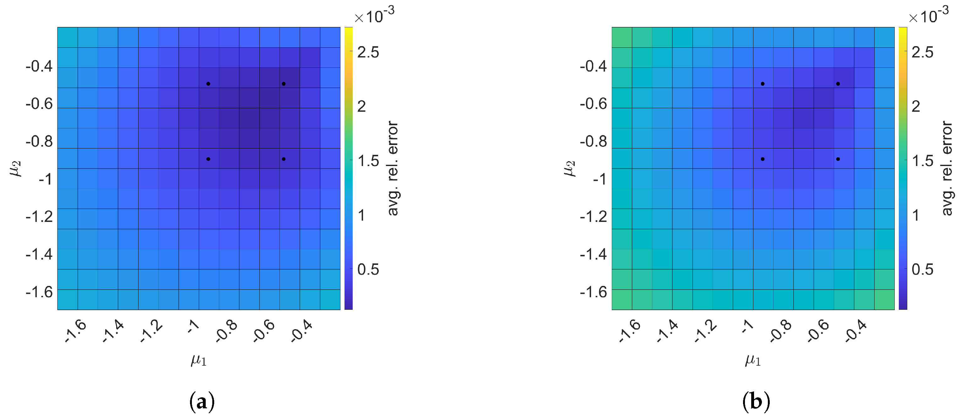
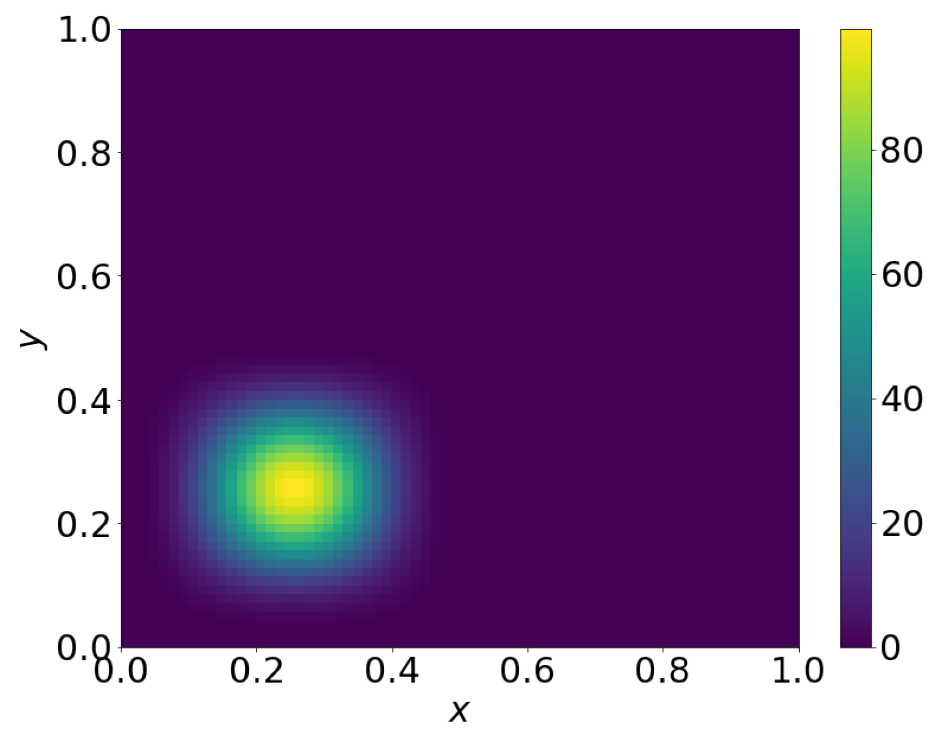
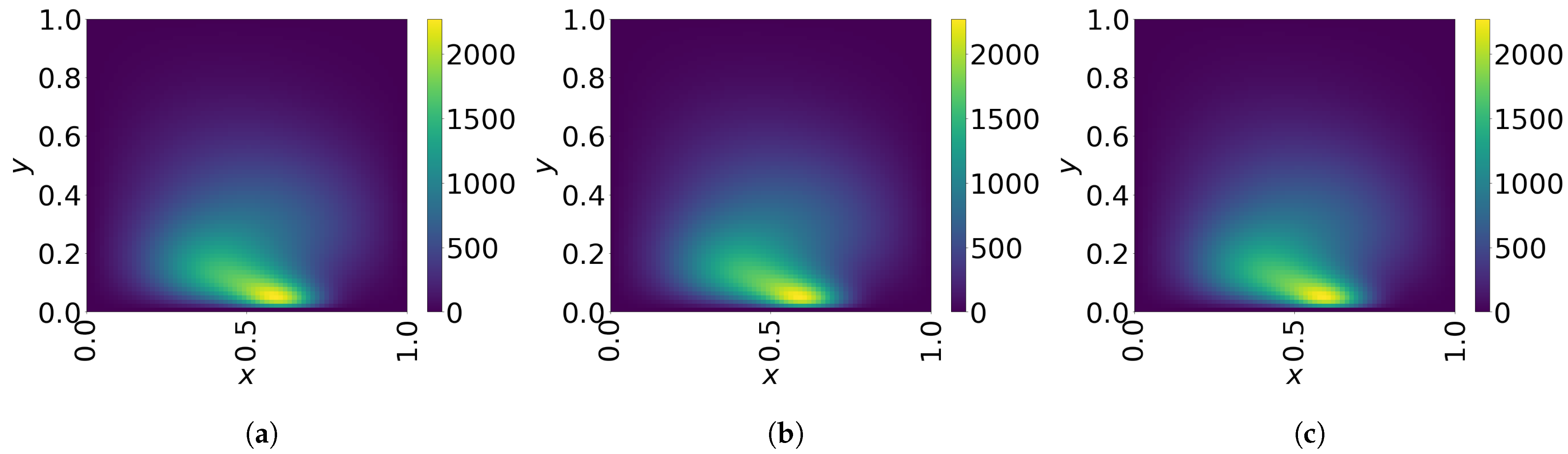
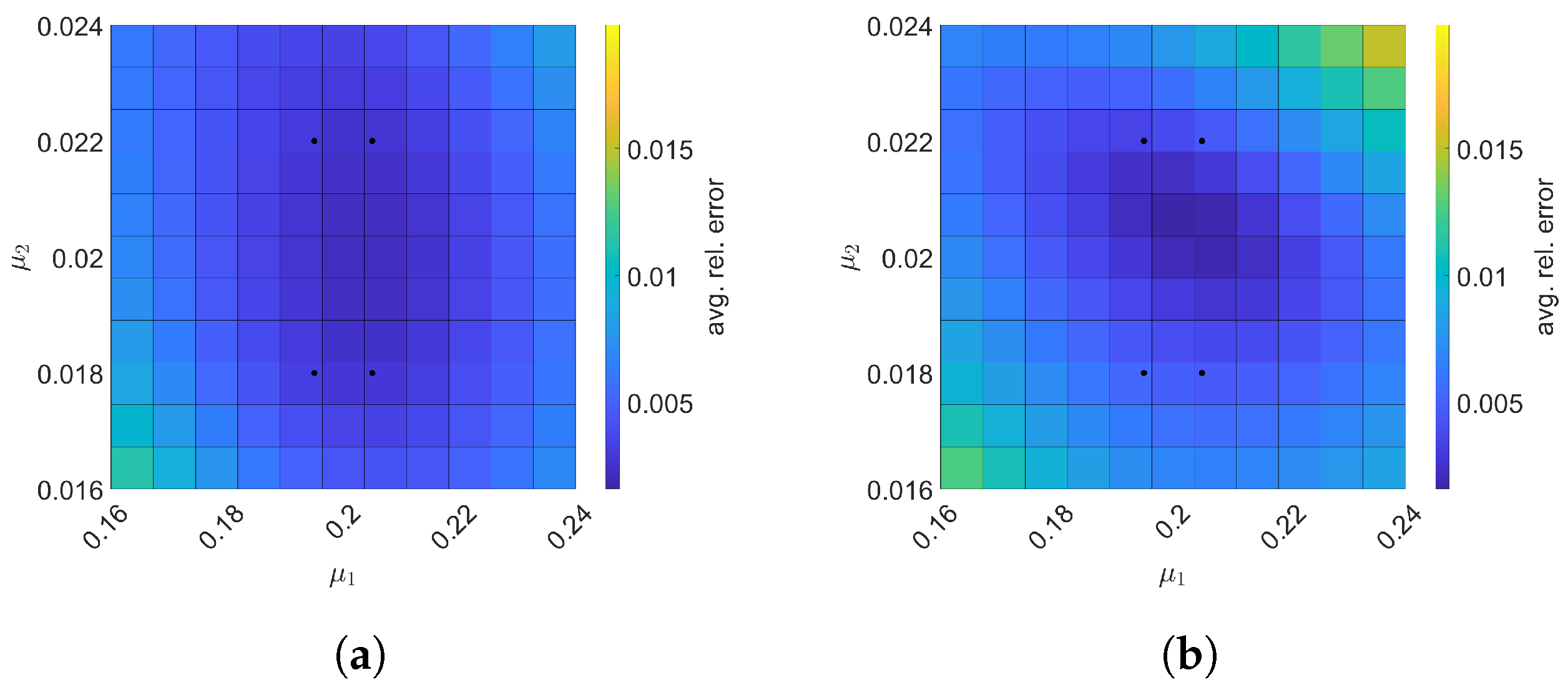
7.1. 2D Linear Diffusion Equation

We consider a parameterized 2D linear diffusion equation with a source term
u t = 2 u x 2 + 2 u y 2 1 ( x μ 1 ) 2 + ( y μ 2 ) 2 u + sin 2 π t ( x μ 1 ) 2 + ( y μ 2 ) 2
where ( x , y ) [ 0 , 1 ] × [ 0 , 1 ] , t [ 0 , 2 ] and ( μ 1 , μ 2 ) [ 1.7 , 0.2 ] × [ 1.7 , 0.2 ] . The boundary condition is
u ( x = 0 , y , t ) = 0 u ( x = 1 , y , t ) = 0 u ( x , y = 0 , t ) = 0 u ( x , y = 1 , t ) = 0
and the initial condition is
u ( x , y , t = 0 ) = 0 .
In Equation (54), the parameters are nonlinearly used in terms of operators, i.e., fractional, so we cannot take advantage of parameter–separability for efficient formation of the reduced order model.
The uniform time step size is given by 2 N t where we set N t = 50 . The space domain is discretized into N x = 70 and N y = 70 uniform meshes in x and y directions, respectively. Excluding boundary grid points, we have N s = ( N x 1 ) × ( N y 1 ) = 4761 spatial degrees of freedom. Multiplying N t and N s gives us 238,050 free degrees of freedom in space–time.
For training phase, we collect solution snapshots associated with the following parameters:
( μ 1 , μ 2 ) { ( 0.9 , 0.9 ) , ( 0.9 , 0.5 ) , ( 0.5 , 0.9 ) , ( 0.5 , 0.5 ) } ,
at which the FOM is solved. The singular value decays of the solution snapshot and the temporal snapshot are shown in Figure 3.
The Galerkin and LSPG space–time ROMs solve the Equation (54) with the target parameter ( μ 1 , μ 2 ) = ( 0.7 , 0.7 ) . Figure 4, Figure 5 and Figure 6 show the relative errors, the space–time residuals, and the online speed-ups as a function of the reduced dimension n s and n t . We observe that both Galerkin and LSPG ROMs with n s = 5 and n t = 3 achieve a good accuracy (i.e., relative errors of 0.012 % and 0.026 % , respectively). However, they are not able to achieve an online speed-up (i.e., 0.082 and 0.073 , respectively) because parameter–separability cannot be made use of. For such problems, local ROM operators can be constructed; then, we can use an interpolation to obtain ROM operator at a certain parameter point. For a detailed description of the local ROM interpolation method, please see [81]. By doing so, online speed-up can be achieved. Excluding assembly time of the FOM and ROM operators from the online phase yields O ( 10 ) solving speed-ups as shown in Figure 7. The Galerkin space–time ROM gives slightly lower relative error than the LSPG space–time ROM (see Figure 4), while the LSPG method gives a slightly lower space–time residual norm than the Galerkin method (see Figure 5), as we repeatedly stated in Section 7.
The final time snapshots of FOM, Galerkin space–time ROM, and LSPG space–time ROM are seen in Figure 8. Both ROMs have a basis size of n s = 5 and n t = 3 , resulting in a reduction factor of ( N s N t ) / ( n s n t ) = 15,870 . For the Galerkin method, the FOM and space–time ROM simulation with n s = 5 and n t = 3 take an average time of 3.9434 × 10 2 and 5.0507 × 10 1 s, respectively, resulting in online speed-up of 0.082 . For the LSPG method, the FOM and space–time ROM simulation with n s = 5 and n t = 3 take an average time of 3.9434 × 10 2 and 5.0507 × 10 1 s, respectively, resulting in speed-up of 0.078 . For accuracy, the Galerkin method results in 1.210 × 10 2 % relative error and 1.249 × 10 2 space–time residual norm, while the LSPG results in 2.626 × 10 2 % relative error and 1.029 × 10 2 space–time residual norm.
Next, we construct space–time ROMs with a basis of n s = 5 and n t = 3 using the same train parameter set given in Equation (57) for solving the predictive cases. The test parameter set is ( μ 1 , μ 2 ) { μ 1 | μ 1 = 1.7 + 1.5 / 14 i , i = 0 , 1 , , 14 } × { μ 2 | μ 2 = 1.7 + 1.5 / 14 j , j = 0 , 1 , , 14 } . Figure 9 shows the relative errors over the test parameter set. The relative errors of both projection methods are the lowest within the rectangular domain defined by the train parameter points, i.e., [ 0.9 , 0.5 ] × [ 0.9 , 0.5 ] . For Galerkin ROM, online speed-up is about 0.088 in average and total time for ROM and FOM are 105.89 and 9.31 s, respectively, resulting in total speed-up of 0.088 . The total time for the ROM consists of 0.13 % of FOM snapshot generation, 0.36 % of ROM basis generation, 99.19 % of ROM operator assembly, and 0.32 % of time integration. For LSPG ROM, online speed-up is about 0.080 in average and total time for ROM and FOM are 114.87 and 9.17 s, respectively, resulting in total speed-up of 0.080 . The breakdown of the total time for the ROM is as follows: 0.12 % of FOM snapshot generation, 0.33 % of ROM basis generation, 99.27 % of ROM operator assembly, and 0.29 % of time integration.

7.2. 2D Linear Convection Diffusion Equation

7.2.1. Without Source Term

We consider a parameterized 2D linear convection diffusion equation
u t = μ 1 u x + u y + μ 2 2 u x 2 + 2 u y 2
where ( x , y ) [ 0 , 1 ] × [ 0 , 1 ] , t [ 0 , 1 ] and ( μ 1 , μ 2 ) [ 0.01 , 0.07 ] × [ 0.31 , 0.37 ] . The boundary condition is given by
u ( x = 0 , y , t ) = 0 u ( x = 1 , y , t ) = 0 u ( x , y = 0 , t ) = 0 u ( x , y = 1 , t ) = 0 .
The initial condition is given by
u ( x , y , t = 0 ) = 100 sin ( 2 π x ) 3 · sin ( 2 π y ) 3 if ( x , y ) [ 0 , 0.5 ] × [ 0 , 0.5 ] 0 otherwise
and shown in Figure 10.
In this example, the parameters are used linearly in terms of operators, thus we can take advantage of parameter–separability for efficient projection of the full order model.
The time domain is discretized with the the uniform time step size 1 N t with N t = 50 . Discretizing the space domain into N x = 70 and N y = 70 uniform meshes in x and y directions, respectively and excluding boundary grid points give us N s = ( N x 1 ) × ( N y 1 ) = 4761 grid points. As a result, there are 238,050 free degrees of freedom in space–time.
For the training phase, we collect solution snapshots associated with the following parameters:
( μ 1 , μ 2 ) { ( 0.03 , 0.33 ) , ( 0.03 , 0.35 ) , ( 0.05 , 0.33 ) , ( 0.05 , 0.35 ) } ,
at which the FOM is solved. Figure 11 shows the singular value decay of the solution snapshot and the temporal snapshot.
The Galerkin and LSPG space–time ROMs solve the Equation (58) with the target parameter ( μ 1 , μ 2 ) = ( 0.04 , 0.34 ) . Figure 12, Figure 13 and Figure 14 show the relative errors, the space–time residuals, and the online speed-ups as a function of the reduced dimension n s and n t . We observe that both Galerkin and LSPG ROMs with n s = 5 and n t = 3 achieve a good accuracy (i.e., relative errors of 0.049 % and 0.059 % , respectively) and speed-up (i.e., 26.52 and 28.59 , respectively). Although the relative errors and space–time residuals are similar, the relative error of Galerkin space–time ROM is slightly lower than the LSPG space–time ROM as shown in Figure 12. On the other hand, Figure 13 shows that the space–time residual of the LSPG method is lower than the Galerkin method.
The final time snapshots of FOM, Galerkin space–time ROM, and LSPG space–time ROM are seen in Figure 15. Both ROMs have a basis size of n s = 5 and n t = 3 , resulting in a reduction factor of ( N s N t ) / ( n s n t ) = 15,870. For the Galerkin method, the FOM and space–time ROM simulation with n s = 5 and n t = 3 takes an average time of 3.4619 × 10 2 and 1.3052 × 10 3 s, respectively, resulting in speed-up of 26.52 . For the LSPG method, the FOM and space–time ROM simulation with n s = 5 and n t = 3 takes an average time of 3.4447 × 10 2 and 1.2049 × 10 3 s, respectively, resulting in speed-up of 28.59 . For accuracy, the Galerkin method results in 4.898 × 10 2 % relative error and 1.503 space–time residual norm while the LSPG results in 5.878 × 10 2 % relative error and 1.459 space–time residual norm.
Now, the space–time reduced order models with n s = 5 and n t = 3 are generated using the same train parameter set given in Equation (61) to solve the predictive cases with the test parameter set, ( μ 1 , μ 2 ) { μ 1 | μ 1 = 0.01 + 0.06 / 11 i , i = 0 , 1 , , 11 } × { μ 2 | μ 2 = 0.31 + 0.06 / 11 j , j = 0 , 1 , , 11 } . Figure 16 shows the relative errors over the test parameter set. The Galerkin and LSPG ROMs are the most accurate within the range of the train parameter points, i.e., [ 0.03 , 0.33 ] × [ 0.05 , 0.35 ] . For Galerkin ROM, online speed-up is about 24.98 in average and total time for ROM and FOM are 1.23 and 5.62 s, respectively, resulting in total speed-up of 4.59 . The total time for the ROM is composed of 10.97 % of FOM snapshot generation, 32.12 % of ROM basis generation, 38.38 % of parameter-independent ROM operator generation, 0.35 % of ROM operator assembly, and 18.18 % of time integration. For LSPG ROM, online speed-up is about 24.79 in average and total time for ROM and FOM are 1.69 and 5.57 s, respectively, resulting in total speed-up of 3.30 . The total time for the ROM breaks down into 7.84 % of FOM snapshot generation, 22.99 % of ROM basis generation, 55.81 % of parameter-independent ROM operator generation, 0.38 % of ROM operator assembly, and 12.97 % time integration.

7.2.2. With Source Term

We consider a parameterized 2D linear convection diffusion equation
u t = μ 1 0.1 u x + u y + μ 2 2 u x 2 + 2 u y 2 + f ( x , y , t )
with the source term f ( x , y , t ) which is given by
f ( x , y , t ) = 10 5 exp ( ( ( x 0.5 + 0.2 sin ( 2 π t ) 0.1 ) 2 + ( y 0.05 ) 2 ) )
where ( x , y ) [ 0 , 1 ] × [ 0 , 1 ] , t [ 0 , 2 ] and ( μ 1 , μ 2 ) [ 0.195 , 0.205 ] × [ 0.018 , 0.022 ] . The boundary condition is given by
u ( x = 0 , y , t ) = 0 u ( x = 1 , y , t ) = 0 u ( x , y = 0 , t ) = 0 u ( x , y = 1 , t ) = 0
and the initial condition is given by
u ( x , y , t = 0 ) = 0 .
Note that the parameters can be factored out when forming reduced order model operators in this example. Thus, we can avoid a lot of re-computation for a parametric case.
For time domain, we set the uniform time step size 2 N t with N t = 50 . For spatial domain, the number of uniform meshes in x and y directions are set N x = 70 and N y = 70 , respectively. Considering free spatial degrees of freedom (i.e., excluding boundary grid points), we have N s = ( N x 1 ) × ( N y 1 ) = 4761 grid points. Then, the number of space–time free degrees of freedom becomes 238,050.
For training phase, we collect solution snapshots associated with the following parameters:
( μ 1 , μ 2 ) { ( 0.195 , 0.018 ) , ( 0.195 , 0.022 ) , ( 0.205 , 0.018 ) , ( 0.205 , 0.022 ) } ,
at which the FOM is solved. In Figure 17, we can see how the singular values of the solution snapshot and the temporal snapshot decay.
The Galerkin and LSPG space–time ROMs solve the Equation (62) with the target parameter ( μ 1 , μ 2 ) = ( 0.2 , 0.02 ) . Figure 18, Figure 19 and Figure 20 show the relative errors, the space–time residuals, and the online speed-ups as a function of the reduced dimension n s and n t . We observe that both Galerkin and LSPG ROMs with n s = 19 and n t = 3 achieve a good accuracy (i.e., relative errors of 0.217 % and 0.265 % , respectively) and speed-up (i.e., 9.18 and 8.54 , respectively). From Figure 18 and Figure 19, we find that there is the same observation that the LSPG method gives lower space–time residuals but higher relative errors as in Section 7.1 and Section 7.2.1.
The final time snapshots of FOM, Galerkin space–time ROM, and LSPG space–time ROM are seen in Figure 21. Both ROMs have a basis size of n s = 19 and n t = 3 , resulting in a reduction factor of ( N s N t ) / ( n s n t ) = 4176. For the Galerkin method, the FOM and space–time ROM simulation with n s = 19 and n t = 3 takes an average time of 3.9159 × 10 2 and 4.2661 × 10 3 s, respectively, resulting in speed-up of 9.18 . For the LSPG method, the FOM and space–time ROM simulation with n s = 19 and n t = 3 takes an average time of 3.6594 × 10 2 and 4.2827 × 10 3 s, respectively, resulting in speed-up of 8.54 . For accuracy, the Galerkin method results in 2.174 × 10 1 % relative error and 1.564 × 10 3 space–time residual norm while the LSPG results in 2.652 × 10 1 % relative error and 1.550 × 10 3 space–time residual norm.
Next, we set the test parameter set to be ( μ 1 , μ 2 ) { μ 1 | μ 1 = 0.160 + 0.08 / 11 i , i = 0 , 1 , , 11 } × { μ 2 | μ 2 = 0.016 + 0.008 / 11 j , j = 0 , 1 , , 11 } . Then, predictive cases with the test parameter set are solved using the space–time ROMs which are generated using the train parameter set given by Equation (66) with n s = 19 and n t = 3 . The relative errors over the test parameter set are shown in Figure 22. We see that the Galerkin and LSPG ROMs are the most accurate inside region of the rectangle defined by the train parameter points, i.e., [ 0.195 , 0.205 ] × [ 0.018 , 0.022 ] . For Galerkin ROM, online speed-up is about 8.94 in average and total time for ROM and FOM are 1.82 and 5.99 s, respectively, resulting in total speed-up of 3.29 . The total time for the ROM breaks down into 7.82 % of FOM snapshot generation, 27.33 % of ROM basis generation, 28.04 % of parameter-independent ROM operator generation, 1.06 % of ROM operator assembly, and 35.75 % of time integration. For LSPG ROM, online speed-up is about 8.94 in average and total times for ROM and FOM are 2.35 and 6.11 s, respectively, resulting in total speed-up of 2.60 . The total time of the ROM consists of 6.59 % of FOM snapshot generation, 22.70 % of ROM basis generation, 41.52 % of parameter-independent ROM operator generation, 1.09 % of ROM operator assembly, and 28.10 % of time integration.

8. Conclusions

In this work, we have formulated Galerkin and LSPG space–time ROMs for linear dynamical systems using block structures which enable us to implement the space–time ROM operators efficiently. We also presented an a posteriori error bound for both Galerkin and LSPG space–time ROMs. We demonstrated that both Galerkin and LSPG space–time ROMs solve 2D linear dynamical systems with parameter–separability accurately and efficiently. Both space–time reduced order models were able to achieve O ( 10 3 ) to O ( 10 4 ) relative errors with O ( 10 ) online speed-ups, and their differences were negligible. We also presented our Python codes used for the numerical examples in Appendix A so that readers can easily reproduce our numerical results. Furthermore, each Python code is less than 120 lines, demonstrating the ease of implementing our space–time ROMs.
We used a linear subspace based ROM which is suitable for accelerating physical simulations whose solution space has a small Kolmogorov n-width. However, the linear subspace based ROM is not able to represent advection-dominated or sharp gradient solutions with a small number of bases. To address this challenge, a nonlinear manifold based ROM can be used, and, recently, a nonlinear manifold based ROM has been developed for spatial ROMs [91,92,93]. In future work, we aim to develop a nonlinear manifold based space–time ROM. Another interesting future direction is to build a component-wise space–time ROM as an extension to the work in [94], which is attractive for extreme-scale problems, whose simulation data are too big to store in a given memory.

Author Contributions

Conceptualization and methodology, Y.C.; coding and validation, Y.K. and K.W.; formal analysis and investigation, Y.K. and K.W.; writing—original draft preparation, Y.K., K.W. and Y.C.; writing—review and editing, Y.K., K.W. and Y.C.; visualization, Y.K.; supervision, Y.C.; project administration, Y.C.; funding acquisition, Y.C. All authors have read and agreed to the published version of the manuscript.

Funding

This work was performed at Lawrence Livermore National Laboratory and was supported by the LDRD program (project 20-FS-007).

Institutional Review Board Statement

Not applicable.

Informed Consent Statement

Not applicable.

Data Availability Statement

All data generated during the current study are available from the corresponding author on reasonable request.

Acknowledgments

We thank four anonymous reviewers whose comments/suggestions helped improve and clarify this manuscript. Youngkyu was supported for this work through generous funding from DTRA. Lawrence Livermore National Laboratory is operated by Lawrence Livermore National Security, LLC, for the U.S. Department of Energy, National Nuclear Security Administration under Contract DE-AC52-07NA27344 and LLNL-JRNL-816093.

Conflicts of Interest

The authors declare no conflict of interest. The funder had a role in the decision to publish the results. The funder had no role in the design of the study, in the collection, analyses, or interpretation of data, or in the writing of the manuscript.

Appendix A. Python Codes in Less than 120 Lines of Code for All Numerical Models Described in Section 7

The Python code used for the numerical examples described in this paper are included in the following pages of the appendix and they are listed below. The total number of lines in each of the files are denoted in the parentheses. Note that we removed print statements of the results:
1.
All input code for the Galerkin Reduced Order Model for 2D Implicit Linear Diffusion Equation with Source Term (111 lines)
2.
All input code for the LSPG Reduced Order Model for 2D Implicit Linear Diffusion Equation with Source Term (117 lines)
3.
All input code for the Galerkin Reduced Order Model for 2D Implicit Linear Convection Diffusion Equation (119 lines)
4.
All input code for the LSPG Reduced Order Model for 2D Implicit Linear Convection Diffusion Equation (119 lines)
5.
All input code for the Galerkin Reduced Order Model for 2D Implicit Linear Convection Diffusion Equation with Source Term (114 lines)
6.
All input code for the LSPG Reduced Order Model for 2D Implicit Linear Convection Diffusion Equation with Source Term (119 lines)

Appendix A.1. Galerkin Reduced Order Model for 2D Implicit Linear Diffusion Equation with Source Term

Mathematics 09 01690 i001a
Mathematics 09 01690 i001b

Appendix A.2. LSPG Reduced Order Model for 2D Implicit Linear Diffusion Equation with Source Term

Mathematics 09 01690 i002a
Mathematics 09 01690 i002b
Mathematics 09 01690 i002c

Appendix A.3. Galerkin Reduced Order Model for 2D Implicit Linear Convection Diffusion Equation

Mathematics 09 01690 i003a
Mathematics 09 01690 i003b

Appendix A.4. LSPG Reduced Order Model for 2D Implicit Linear Convection Diffusion Equation

Mathematics 09 01690 i004a
Mathematics 09 01690 i004b
Mathematics 09 01690 i004c

Appendix A.5. Galerkin Reduced Order Model for 2D Implicit Linear Convection Diffusion Equation with Source Term

Mathematics 09 01690 i005a
Mathematics 09 01690 i005b

Appendix A.6. LSPG Reduced Order Model for 2D Implicit Linear Convection Diffusion Equation with Source Term

Mathematics 09 01690 i006a
Mathematics 09 01690 i006b
Mathematics 09 01690 i006c

References

  1. Mullis, C.; Roberts, R. Synthesis of minimum roundoff noise fixed point digital filters. IEEE Trans. Circuits Syst. 1976, 23, 551–562. [Google Scholar] [CrossRef]
  2. Moore, B. Principal component analysis in linear systems: Controllability, observability, and model reduction. IEEE Trans. Autom. Control 1981, 26, 17–32. [Google Scholar] [CrossRef]
  3. Willcox, K.; Peraire, J. Balanced model reduction via the proper orthogonal decomposition. AIAA J. 2002, 40, 2323–2330. [Google Scholar] [CrossRef]
  4. Willcox, K.; Megretski, A. Fourier series for accurate, stable, reduced-order models in large-scale linear applications. SIAM J. Sci. Comput. 2005, 26, 944–962. [Google Scholar] [CrossRef] [Green Version]
  5. Heinkenschloss, M.; Sorensen, D.C.; Sun, K. Balanced truncation model reduction for a class of descriptor systems with application to the Oseen equations. SIAM J. Sci. Comput. 2008, 30, 1038–1063. [Google Scholar] [CrossRef] [Green Version]
  6. Sandberg, H.; Rantzer, A. Balanced truncation of linear time-varying systems. IEEE Trans. Autom. Control 2004, 49, 217–229. [Google Scholar] [CrossRef] [Green Version]
  7. Hartmann, C.; Vulcanov, V.M.; Schütte, C. Balanced truncation of linear second-order systems: A Hamiltonian approach. Multiscale Model. Simul. 2010, 8, 1348–1367. [Google Scholar] [CrossRef] [Green Version]
  8. Petreczky, M.; Wisniewski, R.; Leth, J. Balanced truncation for linear switched systems. Nonlinear Anal. Hybrid Syst. 2013, 10, 4–20. [Google Scholar] [CrossRef] [Green Version]
  9. Ma, Z.; Rowley, C.W.; Tadmor, G. Snapshot-based balanced truncation for linear time-periodic systems. IEEE Trans. Autom. Control 2010, 55, 469–473. [Google Scholar]
  10. Bai, Z. Krylov subspace techniques for reduced-order modeling of large-scale dynamical systems. Appl. Numer. Math. 2002, 43, 9–44. [Google Scholar] [CrossRef] [Green Version]
  11. Gugercin, S.; Antoulas, A.C.; Beattie, C. H_2 model reduction for large-scale linear dynamical systems. SIAM J. Matrix Anal. Appl. 2008, 30, 609–638. [Google Scholar] [CrossRef]
  12. Astolfi, A. Model reduction by moment matching for linear and nonlinear systems. IEEE Trans. Autom. Control 2010, 55, 2321–2336. [Google Scholar] [CrossRef]
  13. Chiprout, E.; Nakhla, M. Generalized moment-matching methods for transient analysis of interconnect networks. In Proceedings of the 29th ACM/IEEE Design Automation Conference, Anaheim, CA, USA, 8–12 June 1992; pp. 201–206. [Google Scholar]
  14. Pratesi, M.; Santucci, F.; Graziosi, F. Generalized moment matching for the linear combination of lognormal RVs: application to outage analysis in wireless systems. IEEE Trans. Wirel. Commun. 2006, 5, 1122–1132. [Google Scholar] [CrossRef]
  15. Ammar, A.; Mokdad, B.; Chinesta, F.; Keunings, R. A new family of solvers for some classes of multidimensional partial differential equations encountered in kinetic theory modeling of complex fluids. J. Non-Newton. Fluid Mech. 2006, 139, 153–176. [Google Scholar] [CrossRef] [Green Version]
  16. Ammar, A.; Mokdad, B.; Chinesta, F.; Keunings, R. A new family of solvers for some classes of multidimensional partial differential equations encountered in kinetic theory modelling of complex fluids: Part II: Transient simulation using space-time separated representations. J. Non-Newton. Fluid Mech. 2007, 144, 98–121. [Google Scholar] [CrossRef] [Green Version]
  17. Chinesta, F.; Ammar, A.; Cueto, E. Proper generalized decomposition of multiscale models. Int. J. Numer. Methods Eng. 2010, 83, 1114–1132. [Google Scholar] [CrossRef]
  18. Pruliere, E.; Chinesta, F.; Ammar, A. On the deterministic solution of multidimensional parametric models using the proper generalized decomposition. Math. Comput. Simul. 2010, 81, 791–810. [Google Scholar] [CrossRef] [Green Version]
  19. Chinesta, F.; Ammar, A.; Leygue, A.; Keunings, R. An overview of the proper generalized decomposition with applications in computational rheology. J. Non-Newton. Fluid Mech. 2011, 166, 578–592. [Google Scholar] [CrossRef] [Green Version]
  20. Giner, E.; Bognet, B.; Ródenas, J.J.; Leygue, A.; Fuenmayor, F.J.; Chinesta, F. The proper generalized decomposition (PGD) as a numerical procedure to solve 3D cracked plates in linear elastic fracture mechanics. Int. J. Solids Struct. 2013, 50, 1710–1720. [Google Scholar] [CrossRef]
  21. Barbarulo, A.; Ladevèze, P.; Riou, H.; Kovalevsky, L. Proper generalized decomposition applied to linear acoustic: A new tool for broad band calculation. J. Sound Vib. 2014, 333, 2422–2431. [Google Scholar] [CrossRef] [Green Version]
  22. Amsallem, D.; Farhat, C. Stabilization of projection-based reduced-order models. Int. J. Numer. Methods Eng. 2012, 91, 358–377. [Google Scholar] [CrossRef]
  23. Amsallem, D.; Farhat, C. Interpolation method for adapting reduced-order models and application to aeroelasticity. AIAA J. 2008, 46, 1803–1813. [Google Scholar] [CrossRef] [Green Version]
  24. Thomas, J.P.; Dowell, E.H.; Hall, K.C. Three-dimensional transonic aeroelasticity using proper orthogonal decomposition-based reduced-order models. J. Aircr. 2003, 40, 544–551. [Google Scholar] [CrossRef]
  25. Hall, K.C.; Thomas, J.P.; Dowell, E.H. Proper orthogonal decomposition technique for transonic unsteady aerodynamic flows. AIAA J. 2000, 38, 1853–1862. [Google Scholar] [CrossRef]
  26. Simoncini, V. A new iterative method for solving large-scale Lyapunov matrix equations. SIAM J. Sci. Comput. 2007, 29, 1268–1288. [Google Scholar] [CrossRef] [Green Version]
  27. Benner, P.; Li, J.R.; Penzl, T. Numerical solution of large-scale Lyapunov equations, Riccati equations, and linear-quadratic optimal control problems. Numer. Linear Algebra Appl. 2008, 15, 755–777. [Google Scholar] [CrossRef]
  28. Rowley, C.W. Model reduction for fluids, using balanced proper orthogonal decomposition. Int. J. Bifurc. Chaos 2005, 15, 997–1013. [Google Scholar] [CrossRef] [Green Version]
  29. Ma, Z.; Ahuja, S.; Rowley, C.W. Reduced-order models for control of fluids using the eigensystem realization algorithm. Theor. Comput. Fluid Dyn. 2011, 25, 233–247. [Google Scholar] [CrossRef] [Green Version]
  30. Lall, S.; Marsden, J.E.; Glavaški, S. A subspace approach to balanced truncation for model reduction of nonlinear control systems. Int. J. Robust Nonlinear Control. IFAC-Affil. J. 2002, 12, 519–535. [Google Scholar] [CrossRef] [Green Version]
  31. Gosea, I.V.; Gugercin, S.; Beattie, C. Data-driven balancing of linear dynamical systems. arXiv 2021, arXiv:2104.01006. [Google Scholar]
  32. Chinesta, F.; Ladeveze, P.; Cueto, E. A short review on model order reduction based on proper generalized decomposition. Arch. Comput. Methods Eng. 2011, 18, 395. [Google Scholar] [CrossRef] [Green Version]
  33. Mayo, A.; Antoulas, A. A framework for the solution of the generalized realization problem. Linear Algebra Its Appl. 2007, 425, 634–662. [Google Scholar] [CrossRef] [Green Version]
  34. Scarciotti, G.; Astolfi, A. Data-driven model reduction by moment matching for linear and nonlinear systems. Automatica 2017, 79, 340–351. [Google Scholar] [CrossRef]
  35. Schmid, P.J. Dynamic mode decomposition of numerical and experimental data. J. Fluid Mech. 2010, 656, 5–28. [Google Scholar] [CrossRef] [Green Version]
  36. Chen, K.K.; Tu, J.H.; Rowley, C.W. Variants of dynamic mode decomposition: Boundary condition, Koopman, and Fourier analyses. J. Nonlinear Sci. 2012, 22, 887–915. [Google Scholar] [CrossRef]
  37. Williams, M.O.; Kevrekidis, I.G.; Rowley, C.W. A data—Driven approximation of the koopman operator: Extending dynamic mode decomposition. J. Nonlinear Sci. 2015, 25, 1307–1346. [Google Scholar] [CrossRef] [Green Version]
  38. Takeishi, N.; Kawahara, Y.; Yairi, T. Learning Koopman invariant subspaces for dynamic mode decomposition. In Proceedings of the Advances in Neural Information Processing Systems, Long Beach, CA, USA, 4–9 December 2017; pp. 1130–1140. [Google Scholar]
  39. Askham, T.; Kutz, J.N. Variable projection methods for an optimized dynamic mode decomposition. SIAM J. Appl. Dyn. Syst. 2018, 17, 380–416. [Google Scholar] [CrossRef] [Green Version]
  40. Schmid, P.J.; Li, L.; Juniper, M.P.; Pust, O. Applications of the dynamic mode decomposition. Theor. Comput. Fluid Dyn. 2011, 25, 249–259. [Google Scholar] [CrossRef]
  41. Kutz, J.N.; Fu, X.; Brunton, S.L. Multiresolution dynamic mode decomposition. SIAM J. Appl. Dyn. Syst. 2016, 15, 713–735. [Google Scholar] [CrossRef] [Green Version]
  42. Li, Q.; Dietrich, F.; Bollt, E.M.; Kevrekidis, I.G. Extended dynamic mode decomposition with dictionary learning: A data-driven adaptive spectral decomposition of the Koopman operator. Chaos Interdiscip. J. Nonlinear Sci. 2017, 27, 103111. [Google Scholar] [CrossRef]
  43. Proctor, J.L.; Brunton, S.L.; Kutz, J.N. Dynamic mode decomposition with control. SIAM J. Appl. Dyn. Syst. 2016, 15, 142–161. [Google Scholar] [CrossRef] [Green Version]
  44. Tu, J.H.; Rowley, C.W.; Luchtenburg, D.M.; Brunton, S.L.; Kutz, J.N. On dynamic mode decomposition: Theory and applications. arXiv 2013, arXiv:1312.0041. [Google Scholar]
  45. Kutz, J.N.; Brunton, S.L.; Brunton, B.W.; Proctor, J.L. Dynamic Mode Decomposition: Data-Driven Modeling of Complex Systems; SIAM: Philadelphia, PA, USA, 2016. [Google Scholar]
  46. Choi, Y.; Coombs, D.; Anderson, R. SNS: A solution-based nonlinear subspace method for time-dependent model order reduction. SIAM J. Sci. Comput. 2020, 42, A1116–A1146. [Google Scholar] [CrossRef] [Green Version]
  47. Hoang, C.; Choi, Y.; Carlberg, K. Domain-decomposition least-squares Petrov-Galerkin (DD-LSPG) nonlinear model reduction. arXiv 2020, arXiv:2007.11835. [Google Scholar]
  48. Carlberg, K.; Choi, Y.; Sargsyan, S. Conservative model reduction for finite-volume models. J. Comput. Phys. 2018, 371, 280–314. [Google Scholar] [CrossRef] [Green Version]
  49. Berkooz, G.; Holmes, P.; Lumley, J.L. The proper orthogonal decomposition in the analysis of turbulent flows. Annu. Rev. Fluid Mech. 1993, 25, 539–575. [Google Scholar] [CrossRef]
  50. Gubisch, M.; Volkwein, S. Proper orthogonal decomposition for linear-quadratic optimal control. Model Reduct. Approx. Theory Algorithms 2017, 5, 66. [Google Scholar]
  51. Kunisch, K.; Volkwein, S. Galerkin proper orthogonal decomposition methods for parabolic problems. Numer. Math. 2001, 90, 117–148. [Google Scholar] [CrossRef]
  52. Hinze, M.; Volkwein, S. Error estimates for abstract linear—Quadratic optimal control problems using proper orthogonal decomposition. Comput. Optim. Appl. 2008, 39, 319–345. [Google Scholar] [CrossRef]
  53. Kerschen, G.; Golinval, J.C.; Vakakis, A.F.; Bergman, L.A. The method of proper orthogonal decomposition for dynamical characterization and order reduction of mechanical systems: An overview. Nonlinear Dyn. 2005, 41, 147–169. [Google Scholar] [CrossRef]
  54. Bamer, F.; Bucher, C. Application of the proper orthogonal decomposition for linear and nonlinear structures under transient excitations. Acta Mech. 2012, 223, 2549–2563. [Google Scholar] [CrossRef]
  55. Atwell, J.A.; King, B.B. Proper orthogonal decomposition for reduced basis feedback controllers for parabolic equations. Math. Comput. Model. 2001, 33, 1–19. [Google Scholar] [CrossRef]
  56. Rathinam, M.; Petzold, L.R. A new look at proper orthogonal decomposition. SIAM J. Numer. Anal. 2003, 41, 1893–1925. [Google Scholar] [CrossRef]
  57. Kahlbacher, M.; Volkwein, S. Galerkin proper orthogonal decomposition methods for parameter dependent elliptic systems. Discuss. Math. Differ. Inclusions Control Optim. 2007, 27, 95–117. [Google Scholar] [CrossRef] [Green Version]
  58. Bonnet, J.P.; Cole, D.R.; Delville, J.; Glauser, M.N.; Ukeiley, L.S. Stochastic estimation and proper orthogonal decomposition: Complementary techniques for identifying structure. Exp. Fluids 1994, 17, 307–314. [Google Scholar] [CrossRef]
  59. Placzek, A.; Tran, D.M.; Ohayon, R. Hybrid proper orthogonal decomposition formulation for linear structural dynamics. J. Sound Vib. 2008, 318, 943–964. [Google Scholar] [CrossRef] [Green Version]
  60. LeGresley, P.; Alonso, J. Airfoil design optimization using reduced order models based on proper orthogonal decomposition. In Proceedings of the Fluids 2000 Conference and Exhibit, Denver, CO, USA, 19–22 June 2000; p. 2545. [Google Scholar]
  61. Efe, M.O.; Ozbay, H. Proper orthogonal decomposition for reduced order modeling: 2D heat flow. In Proceedings of the 2003 IEEE Conference on Control Applications, (CCA 2003), Istanbul, Turkey, 25–25 June 2003; Volume 2, pp. 1273–1277. [Google Scholar]
  62. Urban, K.; Patera, A. An improved error bound for reduced basis approximation of linear parabolic problems. Math. Comput. 2014, 83, 1599–1615. [Google Scholar] [CrossRef] [Green Version]
  63. Yano, M.; Patera, A.T.; Urban, K. A space-time hp-interpolation-based certified reduced basis method for Burgers’ equation. Math. Model. Methods Appl. Sci. 2014, 24, 1903–1935. [Google Scholar] [CrossRef]
  64. Yano, M. A space-time Petrov–Galerkin certified reduced basis method: Application to the Boussinesq equations. SIAM J. Sci. Comput. 2014, 36, A232–A266. [Google Scholar] [CrossRef]
  65. Baumann, M.; Benner, P.; Heiland, J. Space-time Galerkin POD with application in optimal control of semilinear partial differential equations. SIAM J. Sci. Comput. 2018, 40, A1611–A1641. [Google Scholar] [CrossRef] [Green Version]
  66. Towne, A.; Schmidt, O.T.; Colonius, T. Spectral proper orthogonal decomposition and its relationship to dynamic mode decomposition and resolvent analysis. J. Fluid Mech. 2018, 847, 821–867. [Google Scholar] [CrossRef] [Green Version]
  67. Towne, A. Space-time Galerkin projection via spectral proper orthogonal decomposition and resolvent modes. In Proceedings of the AIAA Scitech 2021 Forum, San Diego, CA, USA, 3–7 January 2021; p. 1676. [Google Scholar]
  68. Towne, A.; Lozano-Durán, A.; Yang, X. Resolvent-based estimation of space–time flow statistics. J. Fluid Mech. 2020, 883. [Google Scholar] [CrossRef] [Green Version]
  69. Choi, Y.; Carlberg, K. Space–Time Least-Squares Petrov–Galerkin Projection for Nonlinear Model Reduction. SIAM J. Sci. Comput. 2019, 41, A26–A58. [Google Scholar] [CrossRef]
  70. Parish, E.J.; Carlberg, K.T. Windowed least-squares model reduction for dynamical systems. J. Comput. Phys. 2021, 426, 109939. [Google Scholar] [CrossRef]
  71. Shimizu, Y.S.; Parish, E.J. Windowed space-time least-squares Petrov-Galerkin method for nonlinear model order reduction. arXiv 2020, arXiv:2012.06073. [Google Scholar]
  72. Choi, Y.; Brown, P.; Arrighi, W.; Anderson, R.; Huynh, K. Space–time reduced order model for large-scale linear dynamical systems with application to Boltzmann transport problems. J. Comput. Phys. 2020, 424, 109845. [Google Scholar] [CrossRef]
  73. Barone, M.F.; Kalashnikova, I.; Segalman, D.J.; Thornquist, H.K. Stable Galerkin reduced order models for linearized compressible flow. J. Comput. Phys. 2009, 228, 1932–1946. [Google Scholar] [CrossRef]
  74. Rezaian, E.; Wei, M. A hybrid stabilization approach for reduced-order models of compressible flows with shock-vortex interaction. Int. J. Numer. Methods Eng. 2020, 121, 1629–1646. [Google Scholar] [CrossRef]
  75. Carlberg, K.; Bou-Mosleh, C.; Farhat, C. Efficient nonlinear model reduction via a least-squares Petrov–Galerkin projection and compressive tensor approximations. Int. J. Numer. Methods Eng. 2011, 86, 155–181. [Google Scholar] [CrossRef]
  76. Huang, C.; Wentland, C.R.; Duraisamy, K.; Merkle, C. Model reduction for multi-scale transport problems using structure-preserving least-squares projections with variable transformation. arXiv 2020, arXiv:2011.02072. [Google Scholar]
  77. Yoon, G.H. Structural topology optimization for frequency response problem using model reduction schemes. Comput. Methods Appl. Mech. Eng. 2010, 199, 1744–1763. [Google Scholar] [CrossRef]
  78. Amir, O.; Stolpe, M.; Sigmund, O. Efficient use of iterative solvers in nested topology optimization. Struct. Multidiscip. Optim. 2010, 42, 55–72. [Google Scholar] [CrossRef]
  79. Amsallem, D.; Zahr, M.; Choi, Y.; Farhat, C. Design optimization using hyper-reduced-order modelsvd. Struct. Multidiscip. Optim. 2015, 51, 919–940. [Google Scholar] [CrossRef]
  80. Gogu, C. Improving the efficiency of large scale topology optimization through on-the-fly reduced order model construction. Int. J. Numer. Methods Eng. 2015, 101, 281–304. [Google Scholar] [CrossRef]
  81. Choi, Y.; Boncoraglio, G.; Anderson, S.; Amsallem, D.; Farhat, C. Gradient-based constrained optimization using a database of linear reduced-order models. J. Comput. Phys. 2020, 423, 109787. [Google Scholar] [CrossRef]
  82. Choi, Y.; Oxberry, G.; White, D.; Kirchdoerfer, T. Accelerating design optimization using reduced order models. arXiv 2019, arXiv:1909.11320. [Google Scholar]
  83. White, D.A.; Choi, Y.; Kudo, J. A dual mesh method with adaptivity for stress-constrained topology optimization. Struct. Multidiscip. Optim. 2020, 61, 749–762. [Google Scholar] [CrossRef]
  84. Najm, H.N. Uncertainty quantification and polynomial chaos techniques in computational fluid dynamics. Annu. Rev. Fluid Mech. 2009, 41, 35–52. [Google Scholar] [CrossRef]
  85. Walters, R.W.; Huyse, L. Uncertainty Analysis for Fluid Mechanics with Applications; Technical Report; National Aeronautics and Space Administration Hampton va Langley Research Center: Hampton, VA, USA, 2002. [Google Scholar]
  86. Zang, T.A. Needs and Opportunities for Uncertainty-Based Multidisciplinary Design Methods for Aerospace Vehicles; National Aeronautics and Space Administration, Langley Research Center: Hampton, VA, USA, 2002. [Google Scholar]
  87. Petersson, N.A.; Garcia, F.M.; Copeland, A.E.; Rydin, Y.L.; DuBois, J.L. Discrete Adjoints for Accurate Numerical Optimization with Application to Quantum Control. arXiv 2020, arXiv:2001.01013. [Google Scholar]
  88. Choi, Y.; Farhat, C.; Murray, W.; Saunders, M. A practical factorization of a Schur complement for PDE-constrained distributed optimal control. J. Sci. Comput. 2015, 65, 576–597. [Google Scholar] [CrossRef] [Green Version]
  89. Choi, Y. Simultaneous Analysis and Design in PDE-Constrained Optimization. Ph.D. Thesis, Stanford University, Stanford, CA, USA, 2012. [Google Scholar]
  90. Sirovich, L. Turbulence and the dynamics of coherent structures. I. Coherent structures. Q. Appl. Math. 1987, 45, 561–571. [Google Scholar] [CrossRef] [Green Version]
  91. Lee, K.; Carlberg, K.T. Model reduction of dynamical systems on nonlinear manifolds using deep convolutional autoencoders. J. Comput. Phys. 2020, 404, 108973. [Google Scholar] [CrossRef] [Green Version]
  92. Kim, Y.; Choi, Y.; Widemann, D.; Zohdi, T. A fast and accurate physics-informed neural network reduced order model with shallow masked autoencoder. arXiv 2020, arXiv:2009.11990. [Google Scholar]
  93. Kim, Y.; Choi, Y.; Widemann, D.; Zohdi, T. Efficient nonlinear manifold reduced order model. arXiv 2020, arXiv:2011.07727. [Google Scholar]
  94. McBane, S.; Choi, Y. Component-wise reduced order model lattice-type structure design. Comput. Methods Appl. Mech. Eng. 2021, 381, 113813. [Google Scholar] [CrossRef]
Figure 1. Illustration of spatial and temporal bases construction, using SVD with n μ = 3 . The right singular vector, v i , describes three different temporal behaviors of a left singular basis vector w i , i.e., three different temporal behaviors of a spatial mode due to three different parameters that are denoted as μ 1 , μ 2 , and μ 3 . Each temporal behavior is denoted as v i 1 , v i 2 , and v i 3 .
Mathematics 09 01690 g001
Figure 2. Growth rate of stability constant in Theorem 1. Backward Euler time stepping scheme with uniform time step size, Δ t = 10 2 is used. (a): ( A st ) 1 2 in inequality (41), (b): Stability constant, η in inequality (41).
Mathematics 09 01690 g002
Figure 3. 2D linear diffusion equation. Graph of singular value decay. (a): Singular value decay of solution snapshot, (b): Singular value decay of temporal snapshot for the first spatial basis vector.
Mathematics 09 01690 g003
Figure 4. 2D linear diffusion equation. Relative errors vs. reduced dimensions. Note that the scales of the z-axis, i.e., the average relative error, are the same both for Galerkin and LSPG. Although the Galerkin achieves slightly lower minimum average relative error values than the LSPG, both Galerkin and LSPG show comparable results. (a): Relative errors vs. reduced dimensions for Galerkin projection, (b): Relative errors vs. reduced dimensions for LSPG projection.
Mathematics 09 01690 g004
Figure 5. 2D linear diffusion equation. Space-time residuals vs. reduced dimensions. Note that the scales of the z-axis, i.e., the residual norm, are the same both for Galerkin and LSPG. Although the LSPG achieves slightly lower minimum residual norm values than the Galerkin, both Galerkin and LSPG show comparable results. (a): Space-time residuals vs. reduced dimensions for Galerkin projection, (b): Space-time residuals vs. reduced dimensions for LSPG projection.
Mathematics 09 01690 g005
Figure 6. 2D linear diffusion equation. Online speed-ups vs. reduced dimensions. Both Galerkin and LSPG show similar speed-ups. (a): Online speed-ups vs. reduced dimensions for Galerkin projection, (b): Online speed-ups vs. reduced dimensions for LSPG projection.
Mathematics 09 01690 g006
Figure 7. 2D linear diffusion equation. Solving speed-ups vs. reduced dimensions. (a): Solving speed-ups vs. reduced dimensions for Galerkin projection, (b): Solving speed-ups vs. reduced dimensions for LSPG projection.
Mathematics 09 01690 g007
Figure 8. 2D linear diffusion equation. Solution snapshots of FOM, Galerkin ROM, and LSPG ROM at t = 2 . (a): FOM, (b): Galerkin ROM, (c): LSPG ROM.
Mathematics 09 01690 g008
Figure 9. 2D linear diffusion equation. The comparison of the Galerkin and LSPG ROMs for predictive cases. The block dots indicate the train parameters. (a): Galerkin, (b): LSPG.
Mathematics 09 01690 g009
Figure 10. Plot of Equation (60).
Mathematics 09 01690 g010
Figure 11. 2D linear convection diffusion equation. Graph of singular value decay. (a): Singular value decay of solution snapshot, (b): Singular value decay of temporal snapshot for the first spatial basis vector.
Mathematics 09 01690 g011
Figure 12. 2D linear convection diffusion equation. Relative errors vs. reduced dimensions. Note that the scales of the z-axis, i.e., the average relative error, are the same both for Galerkin and LSPG. Although the Galerkin achieves slightly lower minimum average relative error values than the LSPG, both Galerkin and LSPG show comparable results. (a): Relative errors vs. reduced dimensions for Galerkin projection, (b): Relative errors vs. reduced dimensions for LSPG projection.
Mathematics 09 01690 g012
Figure 13. 2D linear convection diffusion equation. Space-time residuals vs. reduced dimensions. Note that the scales of the z-axis, i.e., the residual norm, are the same both for Galerkin and LSPG. Although the LSPG achieves slightly lower minimum residual norm values than the Galerkin, both Galerkin and LSPG show comparable results. (a): Space-time residuals vs. reduced dimensions for Galerkin projection, (b): Space-time residuals vs. reduced dimensions for LSPG projection.
Mathematics 09 01690 g013
Figure 14. 2D linear convection diffusion equation. Online speed-ups vs. reduced dimensions. Both Galerkin and LSPG show similar speed-ups. (a): Online speed-ups vs. reduced dimensions for Galerkin projection, (b): Online speed-ups vs. reduced dimensions for LSPG projection.
Mathematics 09 01690 g014
Figure 15. 2D linear convection diffusion equation. Solution snapshots of FOM, Galerkin ROM, and LSPG ROM at t = 1 . (a): FOM, (b): Galerkin ROM, (c): LSPG ROM.
Mathematics 09 01690 g015
Figure 16. 2D linear convection diffusion equation. The comparison of the Galerkin and LSPG ROMs for predictive cases. The block dots indicate the train parameters. (a): Galerkin, (b): LSPG.
Mathematics 09 01690 g016
Figure 17. 2D linear convection diffusion equation with source term. Graph of singular value decay. (a): Singular value decay of solution snapshot, (b): Singular value decay of temporal snapshot for the first spatial basis vector.
Mathematics 09 01690 g017
Figure 18. 2D linear convection diffusion equation with source term. Relative errors vs. reduced dimensions. Note that the scales of the z-axis, i.e., the average relative error, are the same both for Galerkin and LSPG. Although the Galerkin achieves slightly lower minimum average relative error values than the LSPG, both Galerkin and LSPG show comparable results. (a): Relative errors vs. reduced dimensions for Galerkin projection, (b): Relative errors vs. reduced dimensions for LSPG projection.
Mathematics 09 01690 g018
Figure 19. 2D linear convection diffusion equation with source term. Space-time residuals vs. reduced dimensions. Note that the scales of the z-axis, i.e., the residual norm, are the same both for Galerkin and LSPG. Although the LSPG achieves slightly lower minimum residual norm values than the Galerkin, both Galerkin and LSPG show comparable results. (a): Space-time residuals vs. reduced dimensions for Galerkin projection, (b): Space-time residuals vs. reduced dimensions for LSPG projection.
Mathematics 09 01690 g019
Figure 20. 2D linear convection diffusion equation with source term. Online speed-ups vs. reduced dimensions. Both Galerkin and LSPG show similar speed-ups. (a): Online speed-ups vs. reduced dimensions for Galerkin projection, (b): Online speed-ups vs. reduced dimensions for LSPG projection.
Mathematics 09 01690 g020
Figure 21. 2D linear convection diffusion equation with source term. Solution snapshots of FOM, Galerkin ROM, and LSPG ROM at t = 2 . (a): FOM, (b): Galerkin ROM, (c): LSPG ROM.
Mathematics 09 01690 g021
Figure 22. 2D linear convection diffusion equation with source term. The comparison of the Galerkin and LSPG ROMs for predictive cases. The block dots indicate the train parameters. (a): Galerkin, (b): LSPG.
Mathematics 09 01690 g022
Table 1. Comparison of Galerkin and LSPG projections.
GalerkinLSPG
A ^ s t , g ( μ ) = Φ st T A s t ( μ ) Φ st A ^ s t , p g ( μ ) = Φ st T A s t ( μ ) T A s t ( μ ) Φ st
f ^ s t , g ( μ ) = Φ st T f st ( μ ) f ^ s t , p g ( μ ) = Φ st T A s t ( μ ) T f st ( μ )
u ^ 0 s t , g ( μ ) = Φ st T u 0 st ( μ ) u ^ 0 s t , p g ( μ ) = Φ st T A s t ( μ ) T u 0 st ( μ )
Table 2. Comparison of Galerkin and LSPG block structures.
GalerkinLSPG
A ^ s t , g ( μ ) ( j , j ) = A ^ s t , p g ( μ ) ( j , j ) =
k = 1 N t D k j D k j Δ t ( k ) D k j Φ s T A ( μ ) Φ s D k j k = 1 N t D k j Φ s T I N s Δ t ( k ) A ( μ ) T I N s Δ t ( k ) A ( μ ) Φ s D k j
k = 1 N t 1 D k + 1 j D k j + k = 1 N t 1 [ D k j D k j D k j Φ s T I N s Δ t ( k + 1 ) A ( μ ) Φ s D k + 1 j
D k + 1 j Φ s T I N s Δ t ( k + 1 ) A ( μ ) T Φ s D k j ]
f ^ s t , g ( μ ) ( j ) = f ^ s t , p g ( μ ) ( j ) = k = 1 N t D k j Φ s T I N s Δ t ( k ) A ( μ ) T Δ t ( k ) B ( μ ) f ( k ) ( μ )
k = 1 N t D k j Δ t ( k ) Φ s T B ( μ ) f ( k ) ( μ ) k = 1 N t 1 D k j Φ s T Δ t ( k + 1 ) B ( μ ) f ( k + 1 ) ( μ )
u ^ 0 s t , g ( μ ) ( j ) = D 1 j Φ s T u 0 ( μ ) u ^ 0 s t , p g ( μ ) ( j ) = D 1 j Φ s T I N s Δ t ( 1 ) A ( μ ) T u 0 ( μ )
Table 3. Comparison of Galerkin and LSPG computational complexities.
GalerkinLSPG
Not using block structures O ( N s 2 N t n s n t ) O ( N s 2 N t n s n t )
Using block structures O ( N s N t n s n t ) O ( N s N t n s n t )
Publisher’s Note: MDPI stays neutral with regard to jurisdictional claims in published maps and institutional affiliations.

