On the Geometric Description of Nonlinear Elasticity via an Energy Approach Using Barycentric Coordinates

Abstract

The deformation of a solid due to changing boundary conditions is described by a deformation gradient in Euclidean space. If the deformation process is reversible (conservative), the work done by the changing boundary conditions is stored as potential (elastic) energy, a function of the deformation gradient invariants. Based on this, in the present work we built a “discrete energy model” that uses maps between nodal positions of a discrete mesh linked with the invariants of the deformation gradient via standard barycentric coordinates. A special derivation is provided for domains tessellated by tetrahedrons, where the energy functionals are constrained by prescribed boundary conditions via Lagrange multipliers. The analysis of these domains is performed via energy minimisation, where the constraints are eliminated via pre-multiplication of the discrete equations by a discrete null-space matrix of the constraint gradients. Numerical examples are provided to verify the accuracy of the proposed technique. The standard barycentric coordinate system in this work is restricted to three-dimensional (3-D) convex polytopes. We show that for an explicit energy expression, applicable also to non-convex polytopes, the general barycentric coordinates constitute fundamental tools. We define, in addition, the discrete energy via a gradient for general polytopes, which is a natural extension of the definition for discrete domains tessellated by tetrahedra. We, finally, prove that the resulting expressions can consistently describe the deformation of solids.

1. Introduction and Motivation

Computational solid mechanics provides approximate solutions for the deformation of continuous domains subjected to changes in boundary conditions [1,2,3,4,5,6]. The deformation process itself is described by using “intensive quantities”—stresses and strains—and a constitutive relation between them. These quantities have a geometric nature and form continuous tensor fields. The constitutive relation between stresses and strains may vary in the degree of complexity, depending on how the intensive quantities are related to the “extensive quantities”—forces and displacements. For example, the strains can be defined as linearised or nonlinear functions of the displacement gradient, but in all cases they must be symmetric tensors in order to fulfil physical objectivity. On the other hand, stresses can be defined as distributed forces with respect to a specific domain configuration, where the known true or Cauchy stresses are defined with respect to the current/deformed configuration. Furthermore, the simultaneous fulfilment of the balance of linear and angular momenta generates the symmetry of the stress tensor. As a consequence, the differential relations representing the strains as functions of displacements and equilibrium of stresses, together with the constitutive law, form a system of equations, the approximate solution of which is sought either by discretising the underlying solution space or by discretising the operators involved.

For the first approach (discretisation of the solution space), the most prominent example is the well-known finite element method. In this method, the standard finite element formulations, which dominate commercial finite element analysis platforms, are based on a limited number of simple element geometries: triangles and quadrilaterals in 2D, and tetrahedra and hexahedra in 3D. While these are sufficient for most practical problems and make the implementation and the solution quite efficient, there are, however, situations where the use of general polyhedra as the indivisible units covering the domain can be really more advantageous. One obvious example of this kind is related to the representation of large polycrystalline microstructures or cellular assemblies, where the need to insert additional discretisation in the polyhedra may lead to computationally very expensive problems. This has led to developments of finite elements of the form of general polyhedra, including those using an arbitrary number of vertices and faces, those using generally non-convex polyhedra, and those using polyhedra with nonplanar faces [7,8,9]. In parallel, such general polyhedra proved to be the driving force for the recent development of the virtual element method [10,11]. However, to the best of our knowledge, methods that use general polyhedral meshing tools and then employ the subsequent solvers have not become fully established to date, and they remain in the academic domain.

The second approach (discretisation of the operators) is, to a large extent, based on the discrete differential geometry and was kept under development during the last 20 years. In this method, the discrete structure of the analysed solid at a given length-scale is considered as a starting point, i.e., the discretised computational domain is defined via the finite discrete nature of the solid constitution, and can be seen as an assembly of cells of arbitrary sizes and shapes. Concrete examples of this approach put further effort in order to preserve key properties of the system in terms of important invariants, such as energy, by proper discretisation of the operators. Even though these schemes have been well figured out/formulated and tested for a wide range of physical problems involving scalar fields, only a few of them have been proven to be stable when solving solid mechanics problems involving vector fields [12,13,14]. A notable approximation within this approach is the representation of the discrete system with a graph (contour) that allows rather simple formulations for the elasticity [15], the elasto-plasticity [16] and the elasto-plasticity involving damage [17].

For both of the aforementioned approaches in computational solid mechanics, the mesh quality plays crucial role in numerical simulations. For example, in several methods that rely on Voronoi meshes there may appear spurious solutions, mainly due to different scales of edges and faces (presence of small edges and/or faces), see, e.g., in [18] and references therein. Similar problems arising from mesh quality are present in several other methods, see, for example, in [13]. A common approach utilised to overcome such difficulties is the application of re-meshing: an initial tetrahedral mesh of any quality is used to create a new one with improved quality by appropriate merging of neighbouring tetrahedra. Examples of this technique can be found, e.g., in [19], using mesh-free methods, and in [20] using discontinuous Galerkin methods. Such a treatment, however, is not applicable in situations where a mesh representing some physically-based structure is required, e.g., an assembly of polytopes, and possible large differences in scales need to be handled. The effect of scale differences is quite strong due to the representation of differential operators in either approach, and could be overcome by an energy-based formulation.

The main aim of this work, is the consideration of the above open questions, focusing on the derivation of an appropriate energy-based model within the field of computational solid mechanics. This model would combine a continuum geometric description for the stresses and strains in the context of nonlinear elasticity, and a discrete energy formulation for tetrahedra as well as arbitrary convex polyhedra. The paper is structured as follows. We first recall the geometric description of deformation and the continuous definition of elastic (stored, conservative) energy in Section 2. This is subsequently used to derive a discrete energy representation in tetrahedral elements through the use of standard barycentric coordinates, Section 3. The problem of elastic deformation is formulated as an “energy minimisation problem”, where the boundary conditions are imposed via Lagrange multipliers. 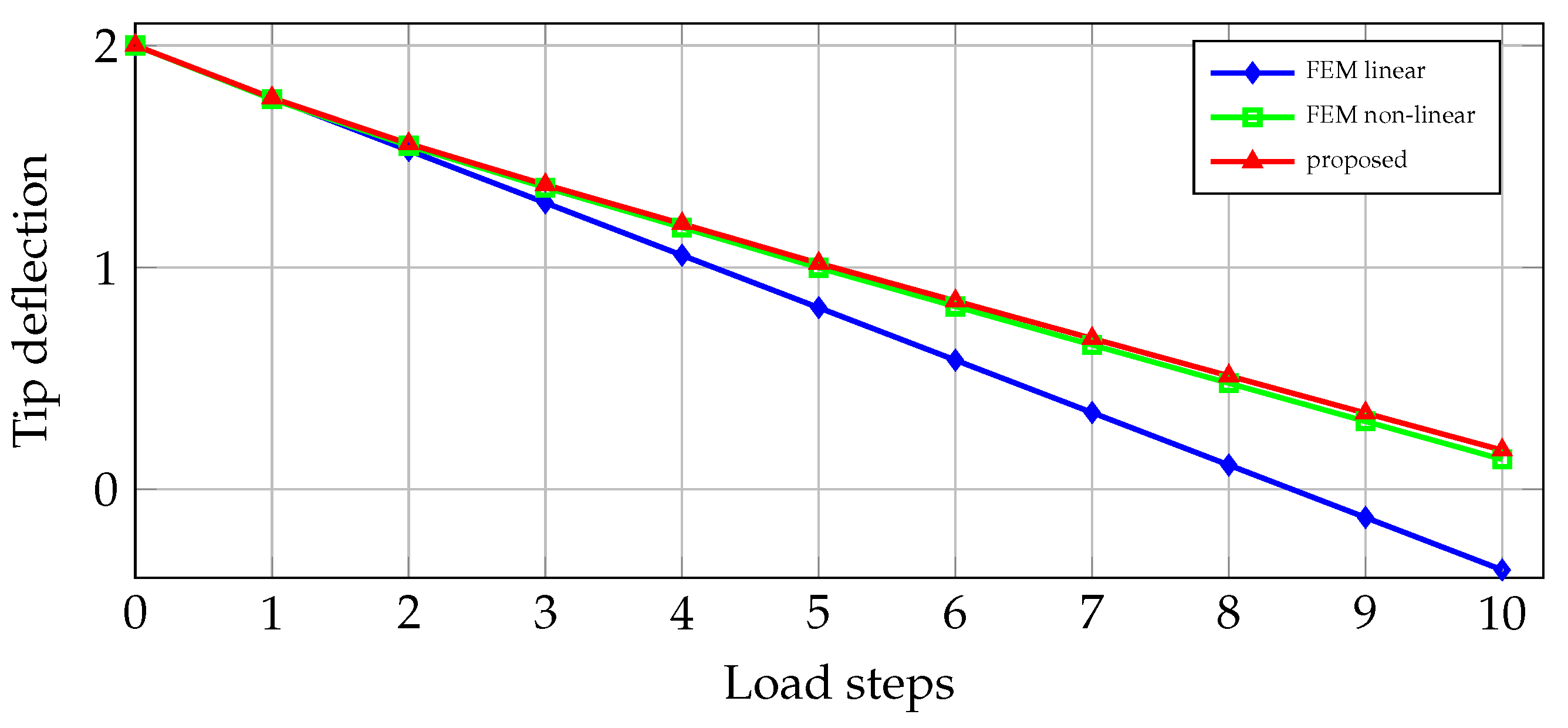The null-space method is then employed to eliminate the Lagrange multipliers, Section 4. 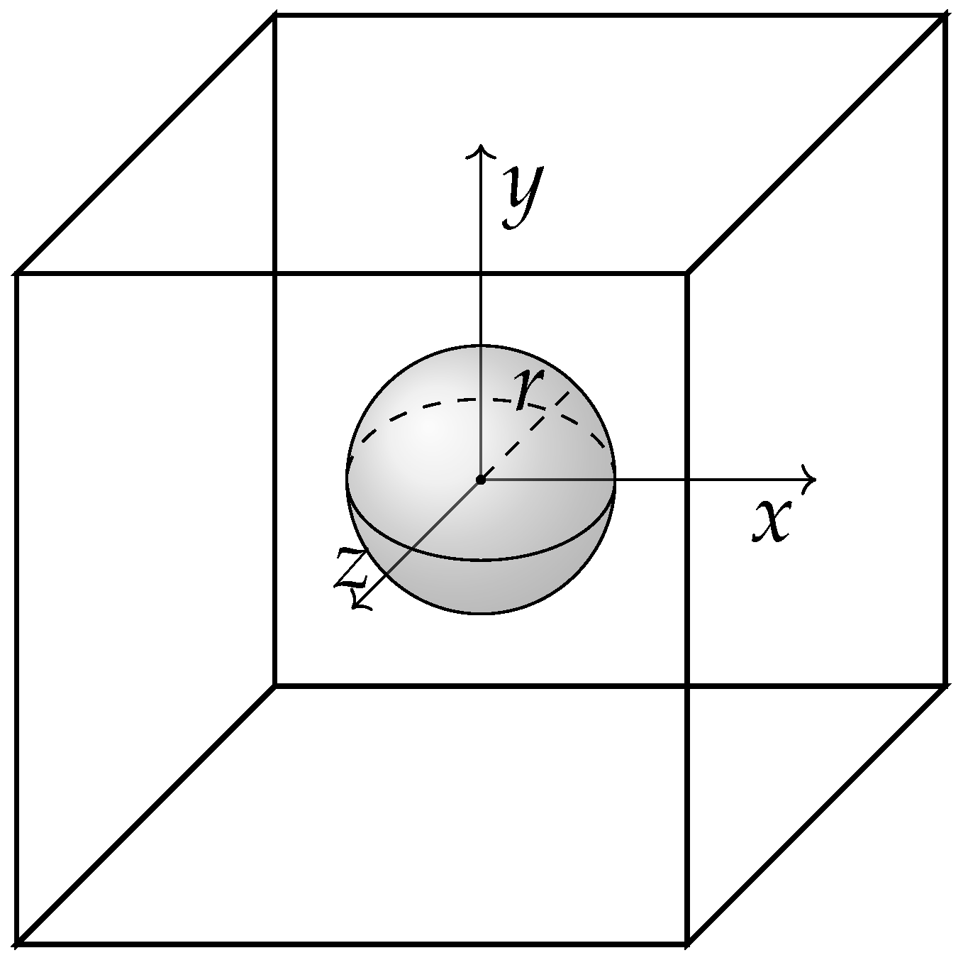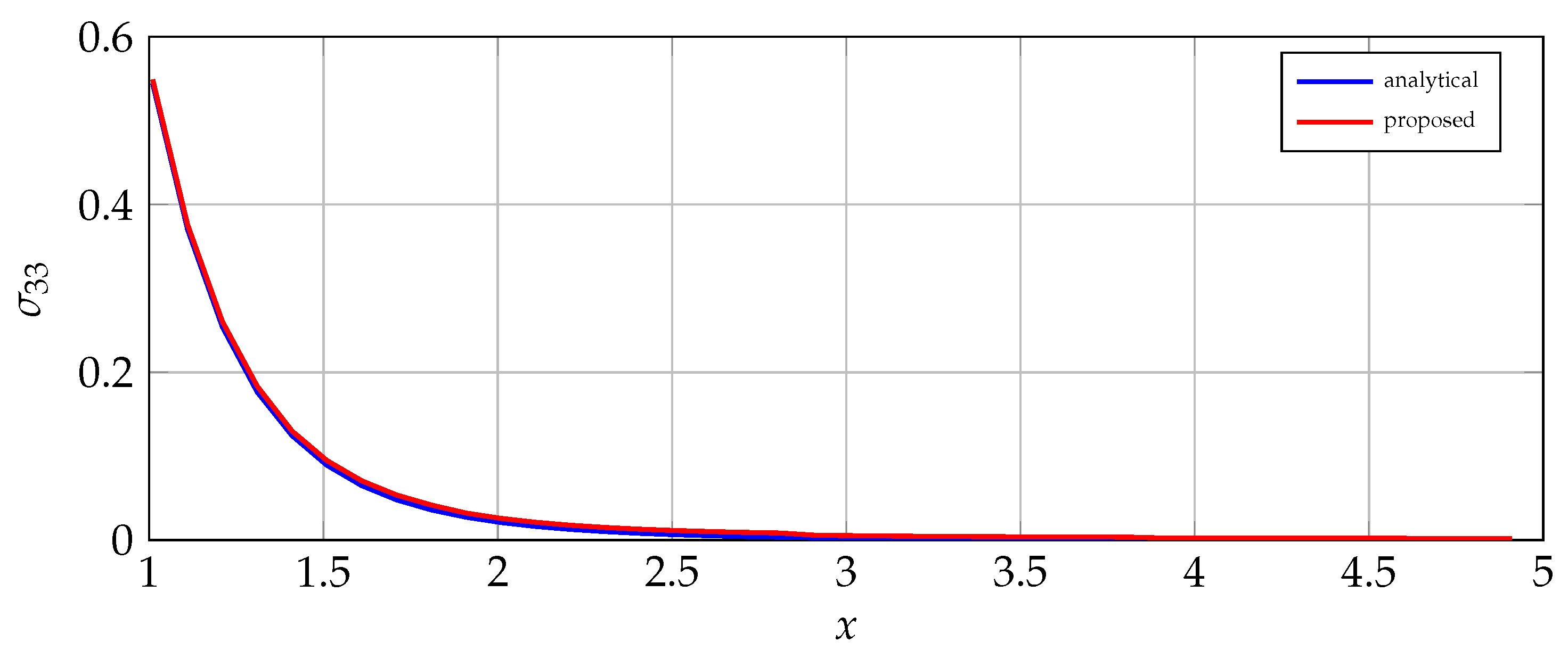The formulation of … and the solution procedure are validated in Section 5 by comparison with analytical solutions for two examples: a cantilever beam subjected to uniformly distributed load, in Section 5.1, and a domain with a spherical hole subjected to remote tension, in Section 5.2. Finally, an energy model for general polytopes is proposed in Section 6. This is achieved by extending the definition of the standard barycentric coordinates to such polytopes, deriving weighted ones, and proving that these can define an energy functional that fully describes the physical system.

2. Deformation and Energy of Conservative Solids

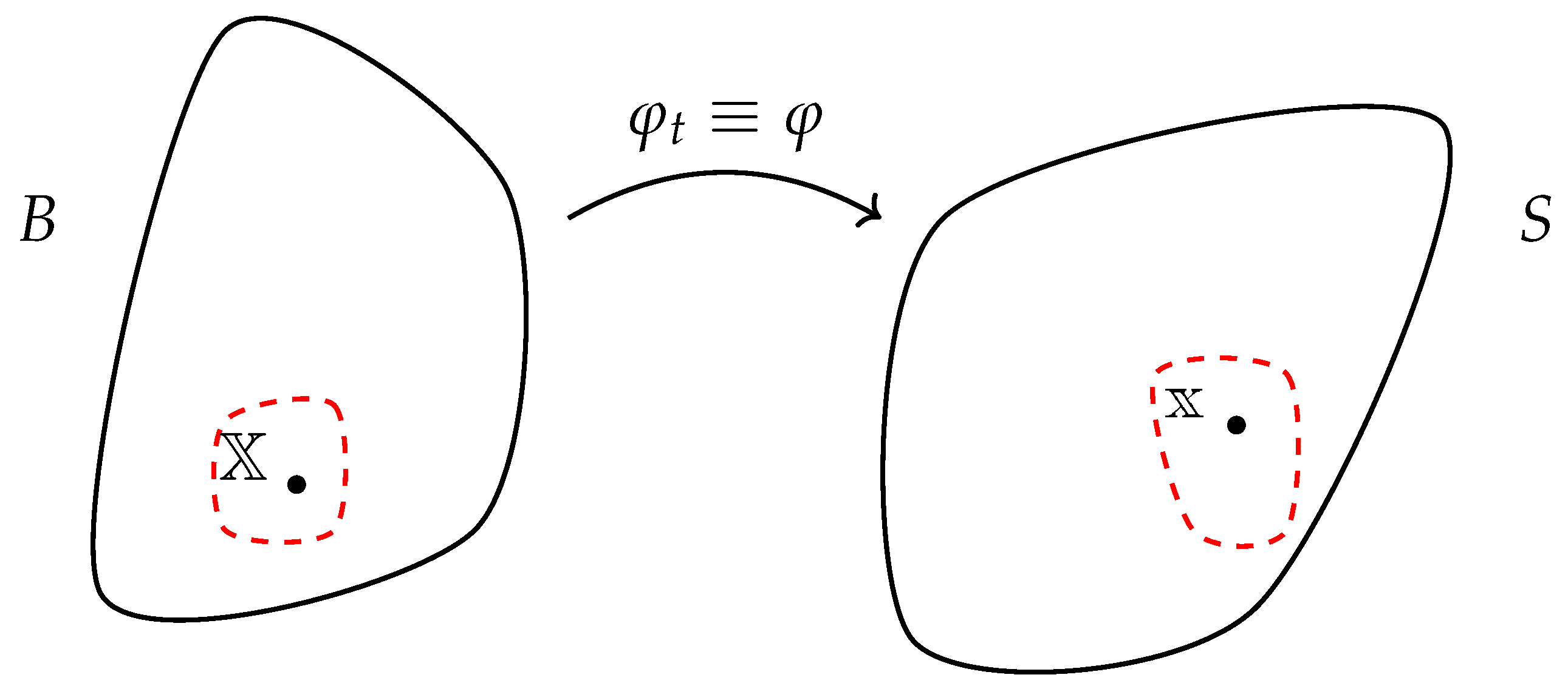
We will first review some of the basic definitions of nonlinear elasticity from a geometric perspective. We start by identifying a material body with a (smooth) Riemannian manifold $ℬ$ and consider a time-dependent deformation of this body to the ambient space Riemannian manifold S described by [1]

$${\phi }_t:B\to {\phi }_t\left(B\right),$$

(1)

or, for simplicity,

$$\phi :B\to S,$$

(2)

see Figure 1. The points within the body are given with their coordinates with respect to a global coordinate system: $\mathbb{X}={\left[X_1{X}_2{X}_3\right]}^T$—in the initial (reference) configuration, and $\mathrm{𝕩}={\left[x_1{x}_2{x}_3\right]}^T$—in the current (deformed) configuration. For these we can rewrite the deformation map (2) as

$$\mathrm{𝕩}=\phi \left(\mathbb{X}\right)\equiv \mathrm{𝕩}\left(\mathbb{X}\right).$$

(3)

The map $\phi$ is considered to be a diffeomorphism, i.e., an invertible differentiable map with differentiable inverse. Manifolds $ℬ$ and S are considered to be equipped with a metric tensor field G. This positive definite second-order tensor field is expressed by symmetric tensors in the tangent space at points of the manifold, denoted by $T_{\mathbb{X}}B$ on $ℬ$ and $T_{\mathrm{𝕩}}S$ on S.

A deformation (3) can also be represented by the deformation gradient $ℱ$, which is the tangent map of $\phi$, i.e., the map between the tangent space on $ℬ$ and the tangent space on S [1,2]:

$$ℱ\left(\mathbb{X}\right):T_{\mathbb{X}}B\to T_{\mathrm{𝕩}}S.$$

(4)

In the local coordinate charts for $\mathbb{X}$ and $\mathrm{𝕩}$, the components ${ℱ}_{ij}$ of $ℱ$ are given by

$${ℱ}_{ij}=\frac{\partial x_i}{\partial X_j}=x_{i,j}\mathrm{for}i,j=1,2,3.$$

(5)

The deformation gradient is a non-singular two-point tensor, i.e., maps the tangent spaces of the two configurations, with a positive determinant, denoted by $\mathbb{J}$. The determinant measures the ratio between the current and initial infinitesimal volume at a given material point, and we note that the condition $\mathbb{J}=1$ represents a volume preserving deformation. $ℱ$ can be multiplicatively decomposed in two possible ways:

$$ℱ=𝒱ℛ=ℛ𝒰,$$

(6)

where $ℛ$ is a proper orthogonal rotation tensor (considering that body and space are of the same Riemannian manifold), and $𝒱$ and $𝒰$ are the so-called left (spatial, current) and right (material, reference) stretch tensors, respectively, which are symmetric positive-definite as $\mathbb{J}>0$. This reflects the two possible representations of the motion: (1) first rotation of a reference unit triad to a current unit triad, followed by its stretching in the current configuration, and (2) stretching of a reference unit triad, followed by rotation to a current triad. The two stretch tensors have identical three positive eigenvalues—${\lambda }_1$, ${\lambda }_2$, and ${\lambda }_3$—representing the principal stretches of the deformation.

In this work, we will consider solids undergoing conservative deformation, i.e., where the solid stores no energy on a complete reversal of the deformation [5]. This behaviour covers the cases of linear and nonlinear elasticity, where all work done on the system by changing boundary conditions from one (initial) to another (current) configuration is stored as an elastic energy, which is exactly equal to the energy required to restore the initial configuration by reversed change of boundary conditions.

An elastic energy formulation in terms of deformation must be invariant with respect to rigid body rotations [1,2,4], thus existing formulations are based on the stretch tensors or some functions of their invariants. We will use one such formulation, which is based on invariants of the so-called left Cauchy–Green strain tensor $ℬ$, given by the map $ℬ\left(\mathrm{𝕩}\right):T_{\mathrm{𝕩}}S\to T_{\mathrm{𝕩}}S$ or by

$$ℬ={𝒱}^2\equiv ℱ{ℱ}^T,$$

(7)

where ${ℱ}^T$ maps covectors in the cotangent bundle of S (or $T^{*}S$) to covectors in the cotangent bundle of B (or $T^{*}B$), see also in [21,22,23,24,25]. It can be easily shown that $ℬ$ is objective, i.e., frame-independent, tensor.

One set of invariants of $ℬ$ is given by [1,2,4]

$$\begin{array}{c}\hfill {\mathbb{I}}_1=tr\left(ℱ{ℱ}^T\right),{\mathbb{I}}_2=\frac{1}{2}\left[{\left(tr\left(ℱ{ℱ}^T\right)\right)}^2-\left(tr{\left(ℱ{ℱ}^T\right)}^2\right)\right],{\mathbb{I}}_3=det\left(ℱ{ℱ}^T\right)={\mathbb{J}}^2\end{array}$$

(8)

which can be written in terms of the three principal stretches as

$$\begin{array}{c}\hfill {\mathbb{I}}_1={\lambda }_1^2+{\lambda }_2^2+{\lambda }_3^2,{\mathbb{I}}_2={\left({\lambda }_1{\lambda }_2\right)}^2+{\left({\lambda }_1{\lambda }_3\right)}^2+{\left({\lambda }_2{\lambda }_3\right)}^2,{\mathbb{I}}_3={\lambda }_1{\lambda }_2{\lambda }_3,\end{array}$$

(9)

Another set of invariants, used to define a large class of non-linear elastic behaviours, is derived from (9) as

$$\begin{array}{c}\hfill {\overline{\mathbb{I}}}_1=\frac{{\mathbb{I}}_1}{{\mathbb{J}}^{2/3}},{\overline{\mathbb{I}}}_2=\frac{{\mathbb{I}}_2}{{\mathbb{J}}^{4/3}},{\overline{\mathbb{I}}}_3=\sqrt{det\left(ℱ{ℱ}^T\right)}=\mathbb{J}.\end{array}$$

(10)

The elastic energy density of a simple generalised Neo-Hookean material is defined in terms of the second set by [2,4]

$$H=\frac{\mu }{2}\left({\overline{\mathbb{I}}}_1-3\right)+\frac{\kappa }{2}{\left(\mathbb{J}-1\right)}^2,$$

(11)

where $\mu$ and $\kappa$ are material-dependent parameters, which in the small strain approximation are known as shear and bulk moduli, respectively.

The integral of the energy density over the solid domain gives the total elastic (stored, potential) energy, which by the principle of stationary action must be minimum for the true deformation; derivation is shown in Appendix A. This can be understood as the system storing the minimal amount of energy for the change of boundary conditions between the initial and the current configuration, or as the change of boundary conditions doing the minimal amount of work (which is equal to the stored energy) to deform the solid from the initial to the current configuration.

While the solid deformation will be formulated as an elastic energy minimisation problem in this work, using the energy density expression (11), the stress tensor will be required for comparisons with known solutions of test problems. The (true) Cauchy stress tensor, $\sigma$, is the derivative of the elastic energy density function with respect to $ℬ$, which for the case of Neo–Hookean materials can be found as

$${\sigma }_{ij}=\frac{\mu }{{\mathbb{J}}^{5/3}}\left({ℬ}_{ij}-\frac{1}{3}{ℬ}_{kk}{\delta }_{ij}\right)+\kappa \left(\mathbb{J}-1\right){\delta }_{ij},$$

(12)

where ${\delta }_{ij}$ is the Kroneckers delta.

Interesting relations between the material parameters and energy can be established via the derivatives of the energy function with respect to the invariants of $ℱ$; these are shown in the Appendix C where the formulation is specialised to linear elasticity, i.e., infinitesimal deformation approximation.

3. Discrete Energy of Tetrahedral Cells

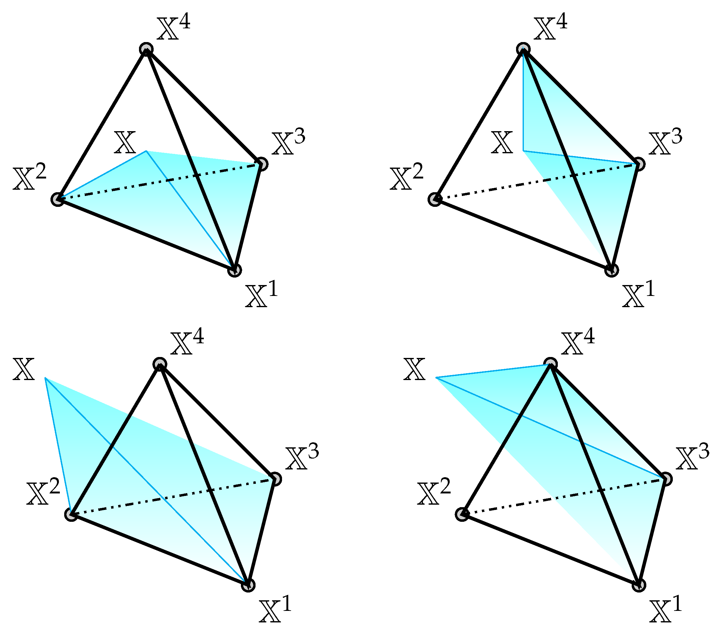
First, we consider a subdivision of the material manifold $ℬ$ into tetrahedra. For a given tetrahedron in ${\mathbb{R}}^3$ with vertices ${\mathbb{X}}^a,{\mathbb{X}}^b,{\mathbb{X}}^c$ and ${\mathbb{X}}^d$, any point $\mathbb{X}$ induces a partition described via

$$\mathbb{X}={\gamma }^a{\mathbb{X}}^a+{\gamma }^b{\mathbb{X}}^b+{\gamma }^c{\mathbb{X}}^c+{\gamma }^d{\mathbb{X}}^d,$$

(13)

where ${\gamma }^a,{\gamma }^b,{\gamma }^c,{\gamma }^d\in \mathbb{R}$ are generalised barycentric coordinates. These are the ratios of the partitioned signed volumes $V_i$ and the tetrahedral volume ($V^t$), see Figure 2. We introduce the vector of barycentric coordinates as

$${\displaystyle ℾ}={\left[\begin{array}{cccc}{\gamma }^a& {\gamma }^b& {\gamma }^c& {\gamma }^d\end{array}\right]}^T.$$

(14)

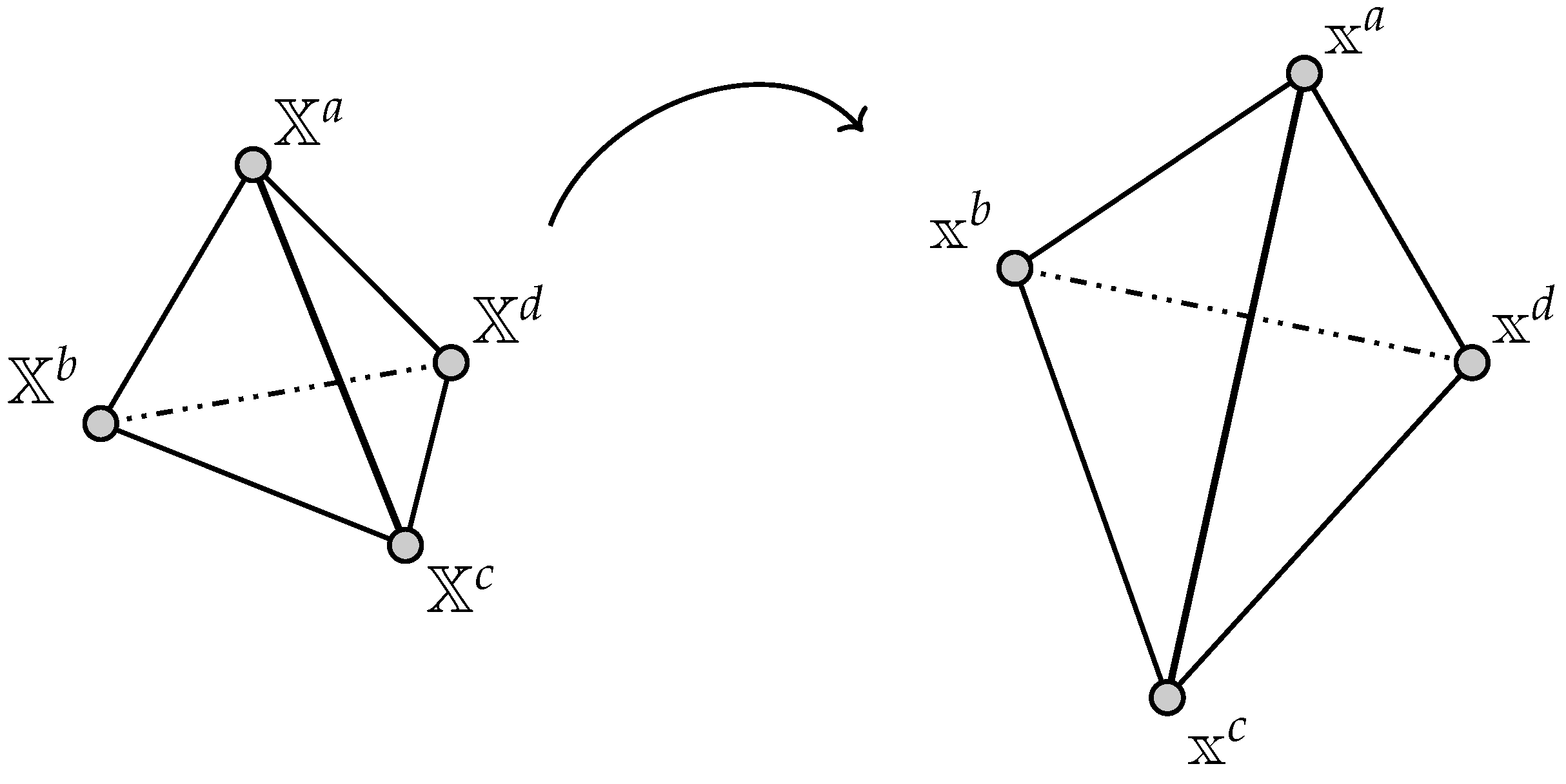
Further, we define a $4\times 4$ matrix $S^r$ describing the tetrahedron shape in the reference configuration by

$$S^r=\left[\begin{array}{cccc}{\tilde{\mathbb{X}}}^a& {\tilde{\mathbb{X}}}^b& {\tilde{\mathbb{X}}}^c& {\tilde{\mathbb{X}}}^d\end{array}\right],$$

(15)

where each column contains corresponding nodal coordinates in the reference system with an additional element “1”, e.g., for the first node we have

$${\tilde{\mathbb{X}}}^a={\left[\begin{array}{cccc}{X}_1^a& X_2^a& X_3^a& 1\end{array}\right]}^T,$$

(16)

and similarly for the remaining three nodes (upper indexes here indicate vertices, see Figure 3, and lower the i-th component of it, $i=1,2,3$). Using this, any point $\mathbb{X}$ in the reference configuration can be expressed by

$$\tilde{\mathbb{X}}=S^r{\displaystyle ℾ}.$$

(17)

Similarly we define a $4\times 4$ matrix $S^d$ describing the tetrahedron shape in the deformed configuration by

$$S^d=\left[\begin{array}{cccc}{\widetilde{\mathrm{𝕩}}}^a& {\widetilde{\mathrm{𝕩}}}^b& {\widetilde{\mathrm{𝕩}}}^c& {\widetilde{\mathrm{𝕩}}}^d\end{array}\right].$$

(18)

Using this, any point $\mathrm{𝕩}$ in the deformed configuration can be expressed by

$$\widetilde{\mathrm{𝕩}}=S^d{\displaystyle ℾ}.$$

(19)

These expressions enable us to define the map between the reference and current configuration for any tetrahedral cell (see Figure 3) by

$$\widetilde{\mathrm{𝕩}}=S^d{\left(S^r\right)}^{-1}\tilde{\mathbb{X}}.$$

(20)

From another side, the physical map between the reference and the current configuration of a tetrahedron can be given by

$$\mathrm{𝕩}=ℱ\mathbb{X}+\mathrm{𝕥},$$

(21)

where $\mathrm{𝕥}=\left[t_i\right],i=1,2,3$ are the components of a translation vector, and $ℱ$ is the deformation gradient which is assumed to have positive determinant.

After some algebra, it can be shown that $S^d{\left(S^r\right)}^{-1}$ is the following a $4\times 4$ block matrix:

$$S^d{\left(S^r\right)}^{-1}=\left[\begin{array}{c}\begin{array}{ll}ℱ& \mathrm{𝕥}\\ {\mathbb{O}}^T& 1\end{array}\end{array}\right],$$

(22)

where $\mathbb{O}$ is a zero vector of size three.

With the knowledge of $ℱ$, the discrete energy of a tetrahedron is calculated by Equation (11), using the invariants given in Equation (10). The sum of energies of all tetrahedrons defines the discrete energy functional of the system.

4. Lagrange Multipliers Using Null-Space Method

When using the discrete energy functional proposed in Section 3 the Euler–Lagrange Equation (A4) are incomplete, and need to be complemented by prescribing Dirichlet (essential) and Neumann (natural) boundary conditions, see Appendix B. For the proposed formulation via energy minimisation, direct application of the boundary conditions is challenging and in such cases Lagrange multipliers have been extensively used [26]. This has been motivated by the fact that both essential and natural boundary conditions can be expressed as constraints and thus enforced by Lagrange multipliers, resulting in the following constrained Euler–Lagrange equations:

$$\frac{d}{d{X}_j}\frac{\partial H}{\partial \left(\partial x_i/\partial X_j\right)}-\frac{\partial H}{\partial x_i}-{\left[C\left(X_j\right)\right]}^T{\lambda }^j=0,$$

(23)

for $i,j=1,2,3$, where $C\left(X_j\right)$ are the constraints and ${\lambda }^j$ are the Lagrange multipliers.

The introduction of Lagrange multipliers increases the number of unknowns, and in order to reduce them to the number of unknown displacements in the system we use the discrete null-space method of [26], which eliminates all Lagrange multipliers. For this, we define a null-space matrix $N\left(X_j\right)$, which satisfies

$$C\left(X_j\right)N\left(X_j\right)=0.$$

(24)

Multiplying from the left with its transpose, Equation (23) becomes

$${\left[N\left(X_j\right)\right]}^T\left(\frac{d}{d{X}_j}\frac{\partial H}{\partial \left(\partial x_i/\partial X_j\right)}-\frac{\partial H}{\partial x_i}\right)=0.$$

(25)

This leads to a number of equations equal to the number of unknown degrees of freedom. Importantly, this technique has been proven to be energy consistent, meaning that energy is neither dissipated nor gained artificially during the numerical process [26,27,28,29,30,31].

5. Numerical Examples

A canonical way to test a proposal for numerical solution of boundary value problems in elasticity is to examine the solution behaviour for several simple deformation modes: volumetric expansion, pure shear, and possibly unconstrained uniaxial extension/compression. While we have tested these modes successfully, the inclusion of the results would not be of significant value to this work. Instead, we provide results for two known elasticity problems, where the combined effect of the different deformation modes is tested: a cantilever beam subjected to a uniformly distributed load and a cube with a spherical hole subjected to tension. We will present and compare results for displacements in the cantilever case, and for stresses in the cube case.

5.1. Cantilever Beam Subjected to a Regular Distributed Load

First, we consider the deformation of a three-dimensional cantilever beam subjected to a uniformly distributed load [4]. The beam has dimensions $10\times 2\times 2$ and is discretised into 5802 tetrahedral elements using 1322 nodes, see Figure 4. The material of the beam has properties $E=3\times {10}^7$ kPa and $\nu =0.3$.

The uniformly distributed load is applied in ten increments with step $f_i=4$ kN/cm${}^2$, and the solution is compared with linear and geometrically nonlinear finite elements analyses performed with identical tetrahedral elements. The comparison shown in Figure 5 illustrates that the calculated deflection is in excellent agreement with the geometrically nonlinear finite element solution. This is the first demonstration that the proposed method based on the minimisation of energy obtained by the barycentric map.

5.2. Cube with a Spherical Hole

Second, we consider the deformation of a cube with a spherical hole subjected to tensile load (Figure 6). The cube dimensions are $20\times 20\times 20$, and the spherical cavity has a radius $r=1$ and centre at the cube centre. Due to symmetries, only one-eight of the cube is considered and tessellated with approximately 100 tetraherdrons. The material properties are the same as in the cantilever example. Uniform tensile load parallel to the x axis is applied.

The problem of a continuum domain with a spherical hole subjected to remote stress has an analytical solution [32]. Specifically the normal stress to the $x,y$ plane ($z=0$) is

$${\sigma }_{33}=\frac{4-5\nu }{2\left(7-5\nu \right)}{\left(\frac{r}{x}\right)}^3+\frac{9}{2\left(7-5\nu \right)}{\left(\frac{r}{x}\right)}^5+1.$$

(26)

This analytical solution is compared with the results obtained with the proposed method in Figure 7: analytical solution is plotted with blue line, calculated stresses are plotted with red line. The demonstrated good agreement between the two lends further support to the proposed approach.

The approach can be tested further against various analytical solutions, but the implementation requires additional work to reduce the computational cost. Additionally, more work must be done on the mesh quality, in order to demonstrate how the number, size and shape of the tetrahedra matter in the calculations. One part of an ongoing work is an implementation of a parallel solver that will massively reduce that time.

6. Discrete Energy on General Polytopes Using Weighted Barycentric Coordinates

In order to define a discrete energy for general three-dimensional elements, we will follow an approach similar to the one described in Section 3. The extension requires first to define general/weighted barycentric coordinates on general polytopes and then to use them to express points of the material domain with respect to the tessellation nodes.

6.1. Standard Barycentric Coordinates Revisited

We start with rewriting the standard barycentric coordinates in a form suitable for generalisation. With respect to a convex polytope with vertices ${\mathbb{X}}_I$ for $I=1,\dots ,n$ (where $n\ge 4$), any point $\mathbb{X}\in {\mathbb{R}}^3$ can written as [33]

$$\mathbb{X}=\sum _{I=1}^n{\gamma }_I{\mathbb{X}}_I,\sum _{I=1}^n{\gamma }_I=1,$$

(27)

where ${\gamma }_I$ are the generalised barycentric coordinates of $\mathbb{X}$. This can be also written in the form

$$\sum _{I=1}^n{w}_I\left({\mathbb{X}}_I-\mathbb{X}\right)=0,\sum _{I=1}^n{w}_I\ne 0,\mathrm{with}{\gamma }_I=\frac{w_I}{{\sum }_{I=1}^n{w}_I},$$

(28)

where the weight functions $w_I$ can be appropriately defined. In [33] for example, the authors define the weight functions via the partition volumes

$$V_I={\{{\mathbb{X}}_1,{\mathbb{X}}_2,\dots ,{\mathbb{X}}_{I-1},\mathbb{X},{\mathbb{X}}_{I+1},\dots ,{\mathbb{X}}_n\}}_{\mathrm{volume}}$$

(29)

and the positive functions $c_I>0$, so that

$$w_I=\frac{c_{I+1}{V}_{I+1}+c_I{V}_I+c_{I-1}{V}_{I-1}}{V_{I+1}{V}_{I-1}}.$$

(30)

The sum of the weight functions becomes

$$W=\sum _{I=1}^n{w}_I=\sum _{I=1}^n\frac{c_{I}V}{V_{I+1}{V}_{I-1}},$$

(31)

where V is the volume of the polytope.

The requirement for $c_I$ is that these are arbitrary positive functions. A rather general definition has been proposed in [33]:

$$c_I={|{\mathbb{X}}_I-\mathbb{X}|}^{\alpha }.$$

(32)

Notably, the selection $\alpha =0$ results in the known Wachspress coordinates, while the selection $\alpha =1$ provides the mean value coordinates.

6.2. Weighted Barycentric Coordinates on General Polytopes

We will now propose an extended version of barycentric coordinates on general polytopes that will be used to formulate an expression of the internal energy. To do so, we use the signed partitioned volumes given by Equation (29) and extend the definition of weight functions given by Equation (31).

Extending the barycentric coordinate expressions to general polytopes is challenging, because one needs to address issues arising from the definition of the weight functions in Equation (31). The problems stem mainly from the denominator, the product of the volumes $V_{I-1}$ and $V_{I+1}$ (or areas in two dimensions). For non-convex polytopes, this product might become negative. In the following, we restrict ourselves to arbitrary (non-platonic) tetrahedral elements, but the generalisation to any general polytope follows clearly. To bypass the possibility of negative denominator, we define the volume using cross-products in the following way:

$$V=\frac{1}{6}\left|\left({\mathbb{X}}_1-{\mathbb{X}}_2\right)\times \left({\mathbb{X}}_1-{\mathbb{X}}_3\right)\right|\left|{\mathrm{𝕙}}_{{\mathbb{X}}_4,({\mathbb{X}}_1,{\mathbb{X}}_2,{\mathbb{X}}_3)}\right|,$$

(33)

where ${\mathrm{𝕙}}_{{\mathbb{X}}_I,({\mathbb{X}}_1,{\mathbb{X}}_2,{\mathbb{X}}_3)}$ is the vector normal to the triangle face forming from points $({\mathbb{X}}_1,{\mathbb{X}}_2,{\mathbb{X}}_3)$ to the point ${\mathbb{X}}_I$.

We can now rewrite the weights of (31) using the proposed volume definition to obtain

$$\begin{array}{ccc}\hfill W& =& \sum _{I=1}^n\frac{6^2{c}_{I}V}{\left|\left({\mathbb{X}}_1-{\mathbb{X}}_2\right)\times \left({\mathbb{X}}_1-{\mathbb{X}}_3\right)\right|\left|{\mathrm{𝕙}}_{\mathbb{X},({\mathbb{X}}_1,{\mathbb{X}}_2,{\mathbb{X}}_3)}\right|\left|\left({\mathbb{X}}_1-{\mathbb{X}}_3\right)\times \left({\mathbb{X}}_1-{\mathbb{X}}_4\right)\right|\left|{\mathrm{𝕙}}_{\mathbb{X},({\mathbb{X}}_1,{\mathbb{X}}_3,{\mathbb{X}}_4)}\right|}\hfill \\ \hfill & =& \sum _{I=1}^n\frac{6c_I\left|{\mathrm{𝕙}}_{{\mathbb{X}}_4,({\mathbb{X}}_1,{\mathbb{X}}_2,{\mathbb{X}}_3)}\right|}{\left|\left({\mathbb{X}}_1-{\mathbb{X}}_3\right)\times \left({\mathbb{X}}_1-{\mathbb{X}}_4\right)\right|\left|{\mathrm{𝕙}}_{\mathbb{X},({\mathbb{X}}_1,{\mathbb{X}}_2,{\mathbb{X}}_3)}\right|\left|{\mathrm{𝕙}}_{\mathbb{X},({\mathbb{X}}_1,{\mathbb{X}}_3,{\mathbb{X}}_4)}\right|}\hfill \\ & =& \sum _{I=1}^n\frac{6c_I\left|{\mathrm{𝕙}}_{{\mathbb{X}}_4,({\mathbb{X}}_1,{\mathbb{X}}_2,{\mathbb{X}}_3)}\right|}{\left|{\mathbb{X}}_1-{\mathbb{X}}_3\right|\left|{\mathbb{X}}_1-{\mathbb{X}}_4\right|\left|{\mathrm{𝕙}}_{\mathbb{X},({\mathbb{X}}_1,{\mathbb{X}}_2,{\mathbb{X}}_3)}\right|\left|{\mathrm{𝕙}}_{\mathbb{X},({\mathbb{X}}_1,{\mathbb{X}}_3,{\mathbb{X}}_4)}\right|sin\left(({\mathbb{X}}_1-{\mathbb{X}}_3),({\mathbb{X}}_1-{\mathbb{X}}_4)\right)},\hfill \end{array}$$

(34)

With some functions $d_I>0$ this can be written as

$$\begin{array}{ccc}\hfill W& =& \sum _{I=1}^n\frac{d_I}{\left|{\mathbb{X}}_1-{\mathbb{X}}_3\right|\left|{\mathbb{X}}_1-{\mathbb{X}}_4\right|sin\left(({\mathbb{X}}_1-{\mathbb{X}}_3),({\mathbb{X}}_1-{\mathbb{X}}_4)\right)}\hfill \\ & =& \sum _{I=1}^n{d}_I\frac{cot\left(({\mathbb{X}}_1-{\mathbb{X}}_3),({\mathbb{X}}_1-{\mathbb{X}}_4)\right)}{\left({\mathbb{X}}_1-{\mathbb{X}}_3\right)·\left({\mathbb{X}}_1-{\mathbb{X}}_4\right)}.\hfill \end{array}$$

(35)

As long as the dot product in the denominator is not zero, the barycentric coordinates that use the proposed weight functions are well defined for both convex and non-convex polytopes. Furthermore, the standard barycentric coordinates can be recovered from this definition.

6.3. Energy from Angles and Lengths

In order to understand more the angles introduced in (35), we will relate them to appropriate lengths of edges. For illustration, we will restrict ourselves to two dimensions, although the extension to three dimensions follows a similar path. We consider the triangle formed by points with coordinates ${\mathbb{X}}_a,{\mathbb{X}}_b$ and ${\mathbb{X}}_c$ (Figure 8). The three angles ${\theta }_a,{\theta }_b$ and ${\theta }_c$ are opposite to the edges of lengths $\left|{\mathrm{𝕙}}_{{\mathbb{X}}_b,{\mathbb{X}}_c}\right|,\left|{\mathrm{𝕙}}_{{\mathbb{X}}_a,{\mathbb{X}}_c}\right|$ and $\left|{\mathrm{𝕙}}_{{\mathbb{X}}_a,{\mathbb{X}}_b}\right|$, respectively.

Considering each angle to be a function of edge lengths, we can write the following expressions:

$$cos\left({\theta }_a\right)=\frac{{\left|{\mathrm{𝕙}}_{{\mathbb{X}}_a,{\mathbb{X}}_c}\right|}^2+{\left|{\mathrm{𝕙}}_{{\mathbb{X}}_a,{\mathbb{X}}_b}\right|}^2-{\left|{\mathrm{𝕙}}_{{\mathbb{X}}_b,{\mathbb{X}}_c}\right|}^2}{2\left|{\mathrm{𝕙}}_{{\mathbb{X}}_a,{\mathbb{X}}_c}\right|\left|{\mathrm{𝕙}}_{{\mathbb{X}}_a,{\mathbb{X}}_b}\right|}.$$

(36)

By taking the derivative with respect to $\left|{\mathrm{𝕙}}_{{\mathbb{X}}_b,{\mathbb{X}}_c}\right|$, we have

$$\frac{\partial {\theta }_a}{\partial \left|{\mathrm{𝕙}}_{{\mathbb{X}}_b,{\mathbb{X}}_c}\right|}=\frac{\left|{\mathrm{𝕙}}_{{\mathbb{X}}_b,{\mathbb{X}}_c}\right|}{\left|{\mathrm{𝕙}}_{{\mathbb{X}}_a,{\mathbb{X}}_c}\right|\left|{\mathrm{𝕙}}_{{\mathbb{X}}_a,{\mathbb{X}}_b}\right|sin\left({\theta }_a\right)},$$

(37)

which, writing the area of the triangle as

$$A=\frac{1}{2}\left|{\mathrm{𝕙}}_{{\mathbb{X}}_a,{\mathbb{X}}_c}\right|\left|{\mathrm{𝕙}}_{{\mathbb{X}}_a,{\mathbb{X}}_b}\right|sin\left({\theta }_a\right)$$

(38)

results in

$$\frac{\partial {\theta }_a}{\partial \left|{\mathrm{𝕙}}_{{\mathbb{X}}_b,{\mathbb{X}}_c}\right|}=\frac{\left|{\mathrm{𝕙}}_{{\mathbb{X}}_b,{\mathbb{X}}_c}\right|}{2A}.$$

(39)

Similarly, we can calculate the derivative of (36) with respect to $\left|{\mathrm{𝕙}}_{{\mathbb{X}}_a,{\mathbb{X}}_c}\right|$ as

$$\frac{\partial {\theta }_a}{\partial \left|{\mathrm{𝕙}}_{{\mathbb{X}}_a,{\mathbb{X}}_c}\right|}=-\frac{\left|{\mathrm{𝕙}}_{{\mathbb{X}}_b,{\mathbb{X}}_c}\right|cos\left({\theta }_c\right)}{2A}.$$

(40)

Finally, to connect the cotangent of an angle, required in (35), we define

$${\xi }_a=\frac{1}{2}{\left|{\mathrm{𝕙}}_{{\mathbb{X}}_b,{\mathbb{X}}_c}\right|}^2,{\xi }_b=\frac{1}{2}{\left|{\mathrm{𝕙}}_{{\mathbb{X}}_a,{\mathbb{X}}_c}\right|}^2,{\xi }_c=\frac{1}{2}{\left|{\mathrm{𝕙}}_{{\mathbb{X}}_a,{\mathbb{X}}_b}\right|}^2$$

(41)

and observe that

$$\frac{\partial cot\left({\theta }_a\right)}{\partial {\xi }_b}=\frac{1}{\left|{\mathrm{𝕙}}_{{\mathbb{X}}_a,{\mathbb{X}}_c}\right|}\frac{\partial cot\left({\theta }_a\right)}{\partial \left|{\mathrm{𝕙}}_{{\mathbb{X}}_a,{\mathbb{X}}_c}\right|}.$$

(42)

The last expression, combined with (40), provides

$$\frac{\partial cot\left({\theta }_a\right)}{\partial {\xi }_b}=\frac{\left|{\mathrm{𝕙}}_{{\mathbb{X}}_b,{\mathbb{X}}_c}\right|cos\left({\theta }_c\right)}{2{sin}^2\left({\theta }_a\right)\left|{\mathrm{𝕙}}_{{\mathbb{X}}_a,{\mathbb{X}}_c}\right|}.$$

(43)

This result gives us a perspective to understand the weights defined by (35) via the derivatives with respect to edge lengths. In addition, due to symmetries we can obtain

$$\frac{\partial cot\left({\theta }_b\right)}{\partial {\xi }_a}=\frac{\left|{\mathrm{𝕙}}_{{\mathbb{X}}_b,{\mathbb{X}}_c}\right|cos\left({\theta }_c\right)}{2{sin}^2\left({\theta }_a\right)\left|{\mathrm{𝕙}}_{{\mathbb{X}}_a,{\mathbb{X}}_c}\right|}$$

(44)

and thus

$$\frac{\partial cot\left({\theta }_a\right)}{\partial {\xi }_b}=\frac{\partial cot\left({\theta }_b\right)}{\partial {\xi }_a}.$$

(45)

The expressions relating cotangent of angles with lengths can be used to formulate an energy expression.

Total energy given by (A2) can be calculated using the energy of any triangle element, i.e., (A1) as

$$h_i\simeq {\int }_{{\xi }_a,{\xi }_b,{\xi }_c}\sum _{I=1}^n{w}_{I}d{\xi }_i\simeq {\int }_{{\xi }_a,{\xi }_b,{\xi }_c}\sum _{a,b,c}cot\left({\theta }_i\right)d{\xi }_i.$$

(46)

6.4. Discrete Energy via Weighted Barycentric Coordinates

We will now prove that the energy expression of (46) can be used to determine the energy at each element. To that end, we here restrict to two-dimensional case, and thus we first prove that the integrant of (46), which can be identified as the differential form

$$\omega =\sum _{a,b,c}cot\left({\theta }_i\right)d{\xi }_i=cot\left({\theta }_a\right)d{\xi }_a+cot\left({\theta }_b\right)d{\xi }_b+cot\left({\theta }_c\right)d{\xi }_c$$

(47)

is a closed 1-form, see in [12,13,14]. The proof can be based on observing that $d\omega$ can be written as

$$\begin{array}{ccc}\hfill d\omega & =& \left[\frac{\partial cot\left({\theta }_b\right)}{\partial {\xi }_a}-\frac{\partial cot\left({\theta }_a\right)}{\partial {\xi }_b}\right]d{\xi }_a\wedge d{\xi }_b\hfill \\ \hfill & & +\left[\frac{\partial cot\left({\theta }_c\right)}{\partial {\xi }_b}-\frac{\partial cot\left({\theta }_b\right)}{\partial {\xi }_c}\right]d{\xi }_b\wedge d{\xi }_c\hfill \\ & & +\left[\frac{\partial cot\left({\theta }_a\right)}{\partial {\xi }_c}-\frac{\partial cot\left({\theta }_c\right)}{\partial {\xi }_a}\right]d{\xi }_c\wedge d{\xi }_a.\hfill \end{array}$$

(48)

To show that $d\omega =0$ is then straightforward using (45).

Finally, the differential form defined in (46) is exact and thus the integration is strictly path-dependent, and thus completely defines an energy functional for the system.

7. Summary and Conclusions

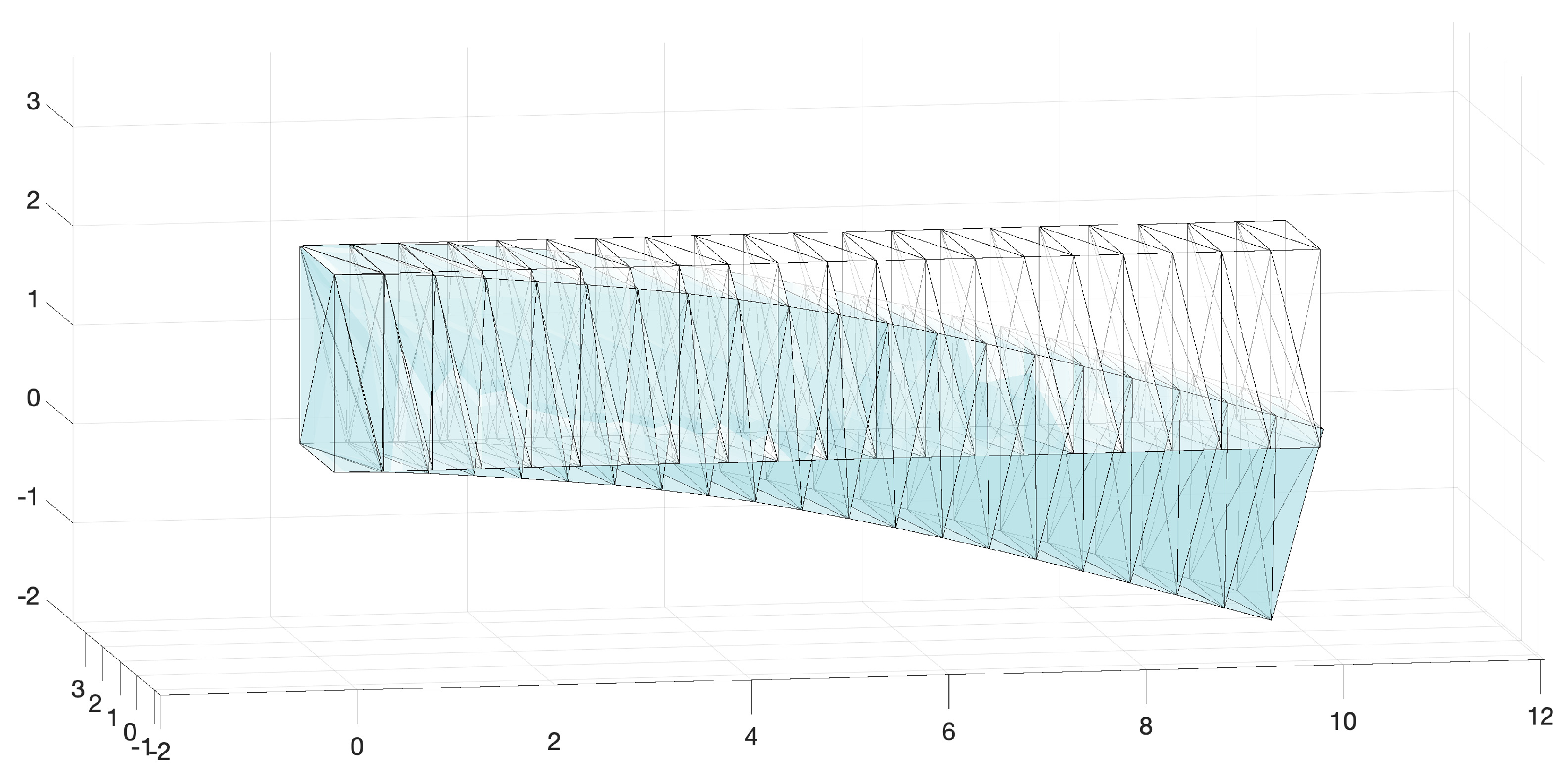
In this work, a geometric formulation of nonlinear elasticity, based on discrete energy functional, is presented. In the first step, discrete energy of tetrahedral elements has been formulated through a map between initial and current positions of their vertices and the use of standard barycentric coordinates. The energy functional of the resulted boundary value problem has been minimised using energy consistent technique for constrained systems, where the constraints are enforced by Lagrange multipliers and are eliminated via pre-multiplication of the discrete equations of motion by a discrete null-space matrix of the constraint gradient. Although not tested specifically here, the convergence of the proposed scheme should inherit the convergence of the well-known methods for solving constrained systems by utilising the discrete null-space method. The numerical examples presented—cantilever beam and cube with a spherical hole—demonstrate the capabilities of the approach.

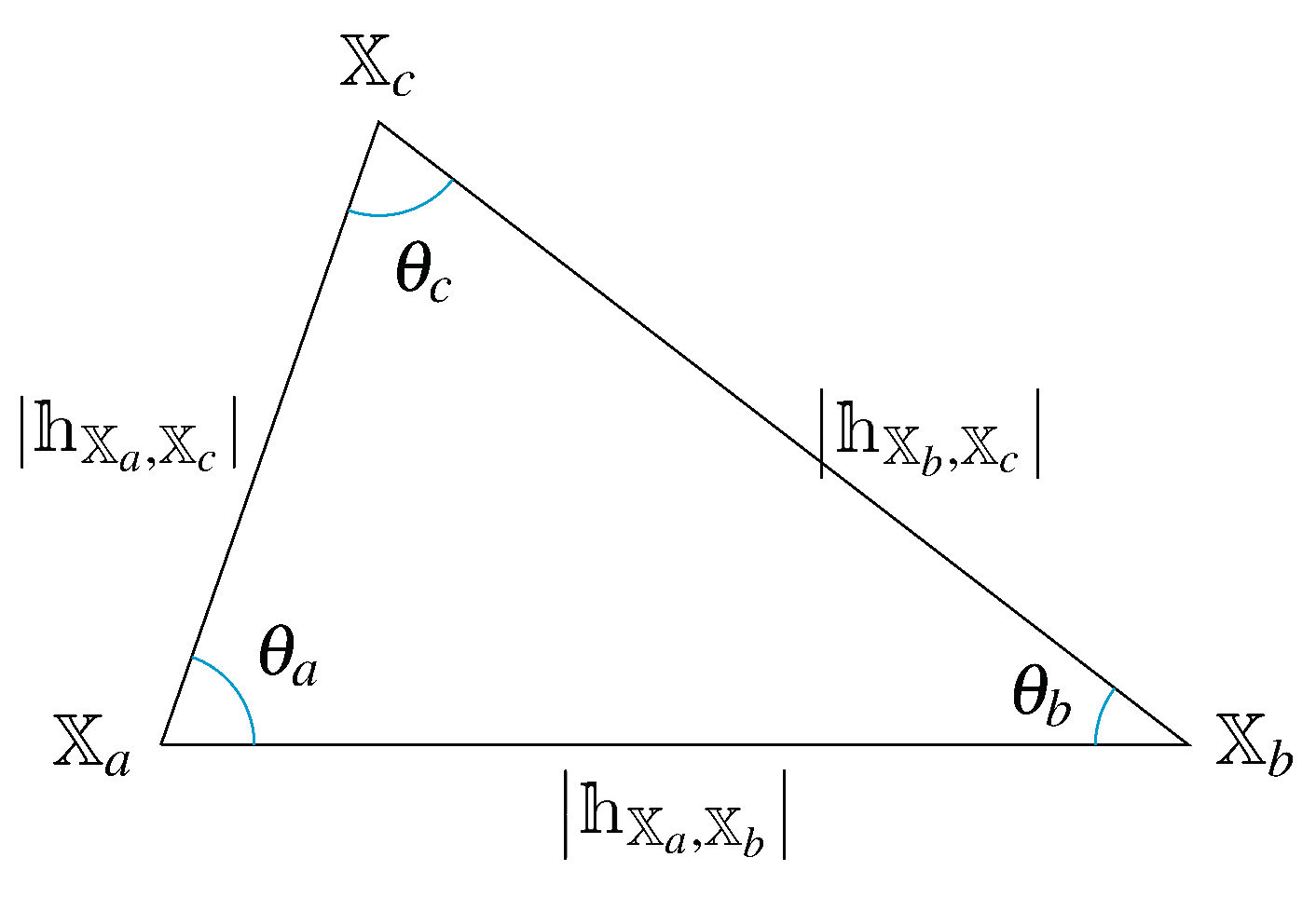
Because the use of standard barycentric coordinates is restricted to three-dimensional convex polytopes, a natural extension of the existing definitions to discrete domains consisting of arbitrary polytopes has been proposed. This opens the possibility to analyse domains with arbitrary cell shapes, including non-convex cells that posses specific microstructural features. The proposed technique is presently suited to conservative problems, i.e., linear and nonlinear elasticity, but it can be extended to dissipative systems, provided that the dissipation mechanism is given in terms of the deformations and stresses calculated in this work. Such extensions are the subject of future work.