Bearing Fault Diagnosis Using a Grad-CAM-Based Convolutional Neuro-Fuzzy Network

Abstract

When a machine tool is used for a long time, its bearing experiences wear and failure due to heat and vibration, resulting in damage to the machine tool. In order to make the machine tool stable for processing, this paper proposes a smart bearing diagnosis system (SBDS), which uses a gradient-weighted class activation mapping (Grad-CAM)-based convolutional neuro-fuzzy network (GC-CNFN) to detect the bearing status of the machine tool. The developed GC-CNFN is composed of a convolutional layer and neuro-fuzzy network. The convolutional layer can automatically extract vibration signal features, which are then classified using the neuro-fuzzy network. Moreover, Grad-CAM is used to analyze the attention of the diagnosis model. To verify the performance of bearing fault classification, the 1D CNN (ODCNN) and improved 1D LeNet-5 (I1DLeNet) were adopted to compare with the proposed GC-CNFN. Experimental results showed that the proposed GC-CNFN required fewer parameters (20K), had a shorter average calculation time (117.7 s), and had a higher prediction accuracy (99.88%) in bearing fault classification. The proposed SBDS can not only accurately classify bearing faults, but also help users understand the current status of the machine tool.

1. Introduction

According to the induction machine failure reports compiled by the Japan Electrical Manufacturers’ Association and IEEE Industry Applications Society, bearing failure is the most common type of machine failure and accounts for 30–40% of all machine failures [1,2,3,4]. Rolling bearings are an indispensable component in induction machines that must function under extreme operating temperatures, under heavy loads, and in harsh high-speed environments. Therefore, rolling bearings are vulnerable to various types of damage. Damage to rolling bearings negatively affects the working of mechanical systems and leads to high financial losses and maintenance costs. To ensure the stable operation of machines, the early detection of new bearing faults is crucial. Data acquisition and mining are helpful to establish the bearing fault diagnosis prediction model [5]. Currently, several bearing fault diagnosis methods, including model-based, signal analysis, and data-driven methods have been proposed.

In model-based fault diagnosis methods, system identification techniques or physical principles are adopted to establish a fault diagnosis system according to the input and output of the practical system. Afshari et al. [6] presented a fault detection technique for rolling-element bearings. This technique involves using a detection filter [7] to detect bearing faults in the inner and outer raceways. Moreover, a sliding mode detector [8] is used to reduce the effects of noise. The simulation results indicated that the aforementioned method can be successfully used to monitor bearing faults. Adams [9] adopted the Lagrange method [10] to establish a mathematical model of a motor system with 29 degrees of freedom for analyzing bearing failure. To validate and parameterize the established model, Adams performed an experiment on a motor. The system response results indicated that the aforementioned model could detect the type of a bearing fault. Jalan [11] developed a fault diagnosis method for rotor bearing systems by using the residual generation technique [12]. Due to the influence of residual vibration, the bearing system was unbalanced and misaligned. The residual force can be analyzed using the equivalent theoretical forces generated by the rotor bearing faults to detect the location and condition of the faults. However, the model-based approach requires experts to design complex mathematical models, and the generalization of developed models is poor.

Signal-based methods usually involve using a vibration signal for bearing fault diagnosis. When a fault occurs, information regarding the fault is reflected in the vibration signal. The faults of a system can be diagnosed by extracting the features of vibration signals. In general, signal-based methods for bearing fault diagnosis can be divided into three categories: time domain, frequency domain, and time–frequency domain methods. Vibration signals can be analyzed in terms of factors such as mean, standard deviation, amplitude, peak, root mean square (RMS), kurtosis, and spectrum. Nikolaou and Antoniadis [13] proposed a wavelet packet analysis with high computational ability and flexibility for identifying faults in rolling-element bearings. Cocconcelli et al. [14] used a short-time Fourier transform (STFT) to analyze residual signals for highlighting the fault effect in the time–frequency domain. A fault was indicated when the sum of the STFT coefficients exceeded the damage threshold. Van et al. [15] developed a hybrid method that combines nonlocal means (NLM) [16,17] and empirical mode decomposition (EMD) [18] for the diagnosis of faults in rolling-element bearings. NLM is used for eliminating noise from the original vibration signal; then, EMD is conducted to detect local faults in rolling bearings. The aforementioned hybrid method was demonstrated to be more efficient than the EMD and discrete wavelet transform methods. Fu et al. [19] employed adaptive fuzzy c-means clustering to recognize different types of bearing faults. First, they extracted vibration signals as eigenvectors that contained information on the RMS, skewness, kurtosis, crest factor, and variance in the time domain. Five parameters were then selected to identify the bearing fault by using fuzzy c-means clustering. The results indicated that adaptive fuzzy c-means clustering can be used to detect the condition of bearings quickly and accurately. Although the aforementioned methods can identify bearing faults, the presence of high noise levels in real environments leads to poor system stability and unfavorable robustness.

Data-driven methods involve using historical data to model systems. In general, data-driven methods require the use of a large quantity of data for model training. In data-driven methods, a model can be established using not only statistical methods but also machine learning methods. Yuwono et al. [20] designed an automatic diagnosis system by using a hidden Markov model (HMM) and swarm rapid centroid estimation for bearing fault identification. The frequency features extracted through wavelet kurtogram analysis and cepstral liftering were used to diagnose bearing faults according to the HMM. The experimental results of the aforementioned authors indicated that their system can effectively diagnose fault types. Ali et al. [21] presented a monitoring system for the diagnosis of faults in rolling bearings. This system performs feature extraction according to the EMD energy entropy. The extracted features are then used to train an ANN for classifying bearings faults. The results of Ali et al. indicated that their monitoring system can reliably categorize bearing faults and ensure the steadiness of machinery. Ertunc et al. [22] compared the bearing fault detection performance of the ANN and adaptive neuro-fuzzy inference system (ANFIS) [23] models. They used different filters, such as bandpass and low-pass filters, to capture the characteristics of the vibration signal in the time and frequency domains for training the ANN and ANFIS models. Test results revealed that the fault diagnosis accuracy of the ANFIS model was higher than that of the ANN model. Devisi et al. [24] used zSlice type-2 fuzzy sets to overcome the shortcomings of type-1, which cannot deal with uncertainty problems. On the other hand, it also improves the complexity of the traditional type 2 fuzzy logic system and the huge computational requirements. Although the aforementioned methods are more accurate and flexible than model- and signal-based methods are, the aforementioned methods rely on manual feature extraction, which is tedious and considerably affects the final result. If the quality of the extracted features is poor, the accuracy of the model is low.

Some scholars have used deep learning for bearing fault detection. The most commonly used deep learning architecture is the CNN, which comprises a convolution layer, pooling layer, and fully connected layer. Zhang et al. [25] designed a deep CNN with wide first-layer kernels for bearing fault diagnosis. The influence of different convolutional kernel sizes on the accuracy was also investigated in the aforementioned research. The aforementioned authors revealed that the accuracy increased with kernel size; however, a large kernel size is unsuitable for extracting local features. Wen et al. [26] adopted LeNet-5 for bearing fault diagnosis. They converted one-dimensional (1D) time-domain raw vibration signals into two-dimensional (2D) images by using a signal-to-image conversion method developed by them. The converted images, which were 64 × 64 pixels in size, were used for training LeNet-5. The results indicated that LeNet-5 had a higher fault prediction accuracy than did other traditional methods, such as support vector machine [27], sparse filter [28], and deep belief network approaches [29]. In addition, Wen et al. indicated that deep learning involves the use of a large number of parameters, which makes the training process time-consuming. Xie et al. [30] designed a 1D CNN (ODCNN) to detect faults in rolling bearings. Their experimental results indicated that the ODCNN achieved high accuracy in bearing fault classification. Wan et al. [31] proposed and compared the bearing fault diagnosis performance of the improved 1D LeNet-5 (I1DLeNet) and improved 2D LeNet-5 (I2DLeNet) models. The I1DLeNet model uses raw vibration signals as inputs. The I2DLeNet model uses grayscale images transformed from raw vibration signals through histogram equalization as inputs. The Case Western Reserve University (CWRU) bearing dataset was used to verify the aforementioned two models. The results indicated that the I1DLeNet model is superior to the I2DLeNet model for the diagnosis of faults in rolling-element bearings. Numerous studies have indicated that compared with traditional methods, deep learning methods have superior automatic feature extraction and provide more accurate predictions. Nevertheless, the existence of a large number of trainable parameters in deep learning methods means that expensive GPU hardware is required to accelerate calculations.

The aforementioned literature methods indicate that bearing failure can be successfully diagnosed. However, those methods have certain disadvantages, such as that (1) system stability and robustness are poor, (2) experts are required to extract features manually, and (3) users spend a lot of time training huge network parameters. How to design a bearing fault diagnosis system that is fast, effective, and has few hardware resources was the aim of this study. In this study, a smart bearing diagnosis system (SBDS) based on the Grad-CAM-based CNFN (GC-CNFN) for bearing fault diagnosis is proposed. The contributions of this study include the following:

(1)

A novel SBDS was developed to diagnose the health of bearing.

(2)

A high-precision GC-CNFN model with fewer parameters is proposed to identify bearing faults.

(3)

The proposed GC-CNFN can automatically perform feature extraction from and modeling with the original raw vibration signal without the need for expert experience and knowledge.

(4)

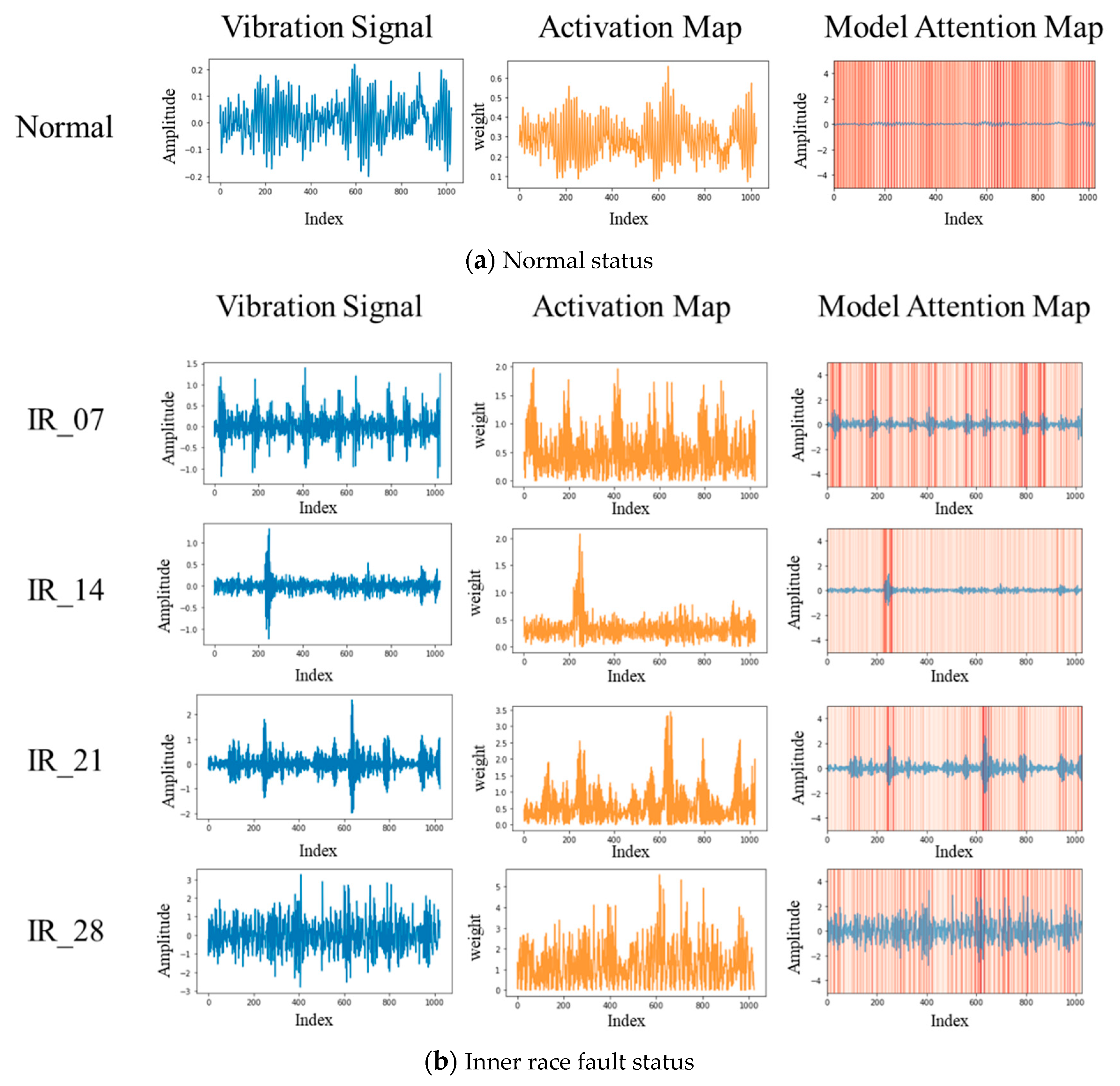
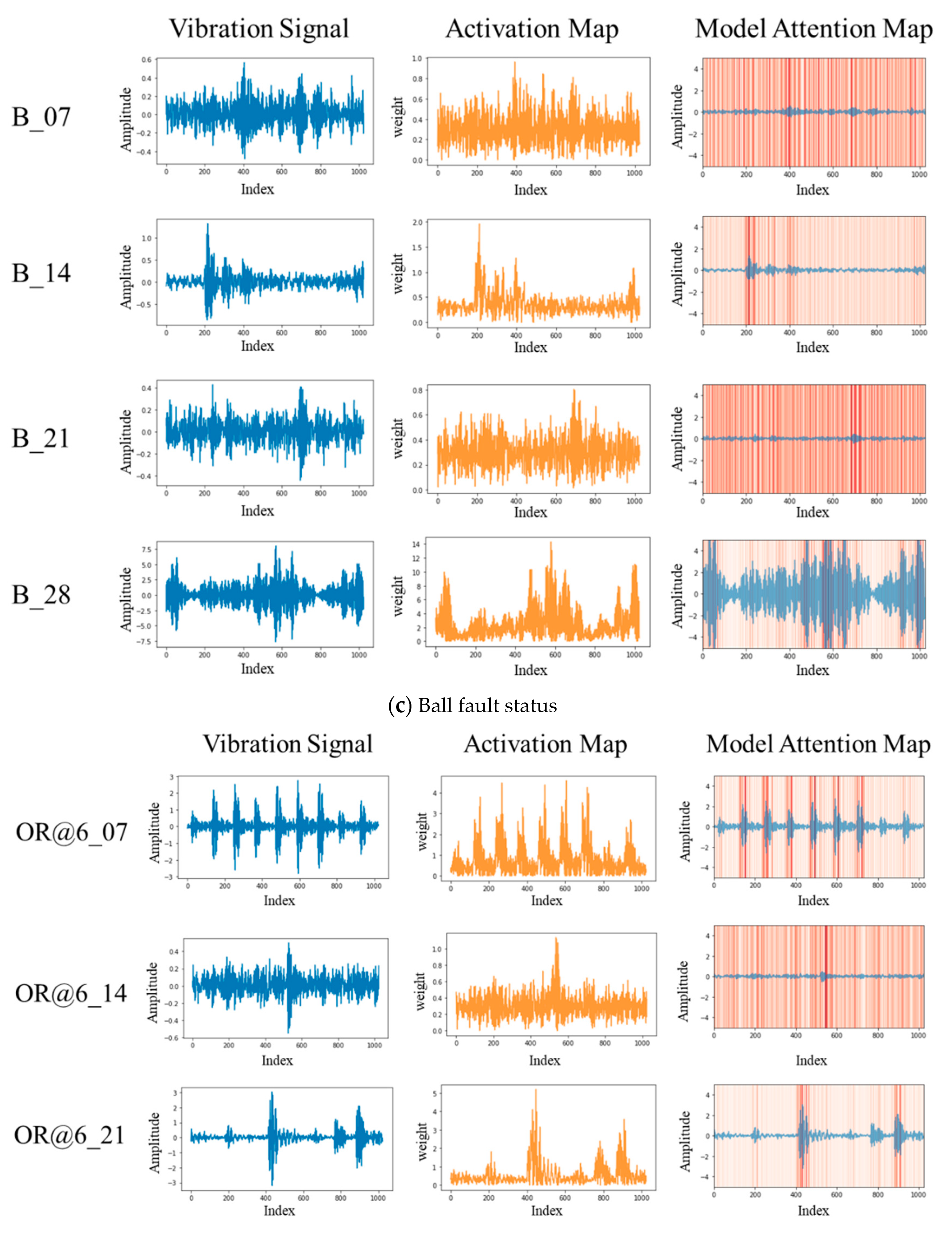
By referring to the model attention maps generated by the GC-CNFN, users can determine the region in which the model focuses on the vibration signal and understand the basis of the model’s classification.

The remainder of this paper is organized as follows. Section 2 describes the related works of CNN and Grad-CAM. The designed SBDS is described for bearing fault diagnosis in Section 3. Section 4 presents the experimental results obtained when using the designed SBDS. Finally, Section 5 presents the conclusions of this study and recommendations for future research.

2. Related Work

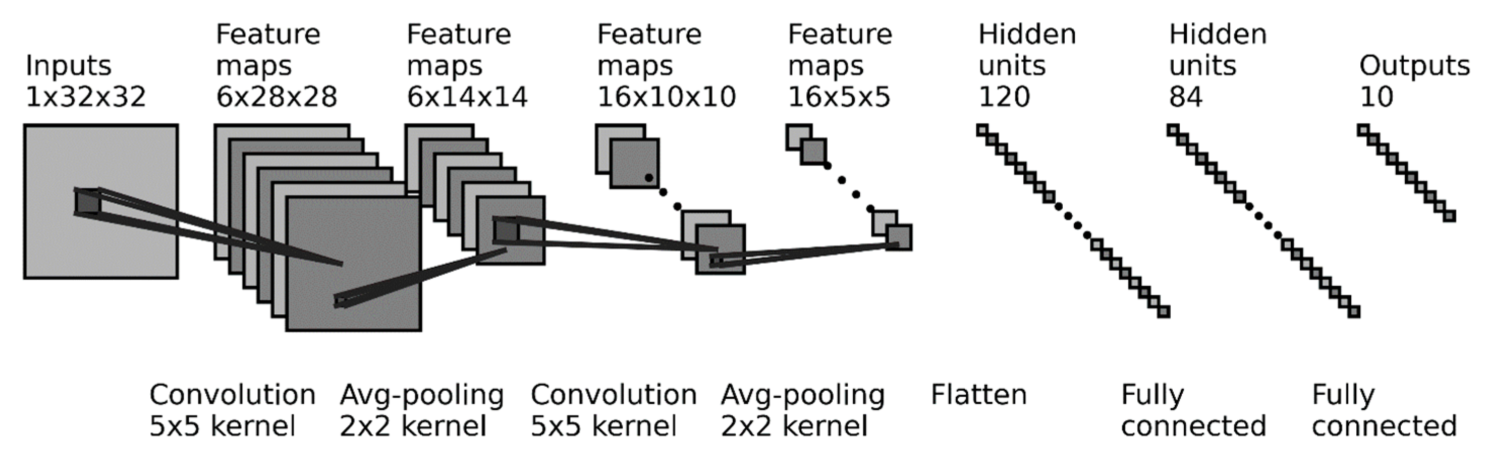
2.1. Convolutional Neural Network (CNN)

In this section, the classic CNN architecture of LeNet-5 [32], which was invented by LeCun, is described. The architecture of LeNet-5 is displayed in Figure 1. As displayed in Figure 1, LeNet-5 comprises two convolution layers, two pooling layers, a flatten layer, and two fully connected layers.

The operation of each layer is described in detail as follows:

• Convolution layer

A convolution layer [33,34] contains several convolution kernels for convolving input local regions. The convolved results are passed through a sigmoid function to obtain feature maps. The convolution operation involves performing an element-wise product operation on the input and the convolution kernel in a sliding window. The equation of the convolution operation is presented in Equation (1).

$$C_{xy}^j=\sigma \left({{\displaystyle \sum }}_{i=1}^n{{\displaystyle \sum }}_{u=0}^{k_h-1}{{\displaystyle \sum }}_{v=0}^{k_w-1}{I}_{\left(\left(x+u\right),\left(y+v\right)\right)}^i{w}_{\left(u,v\right)}^{ij}+b^j\right)$$

(1)

$$\sigma \left(x\right)=\frac{1}{1+e^{-x}}$$

(2)

where $C_{xy}^j$ presents the jth feature map at position $\left(x,y\right)$; n is the number of input channels; $k_h$ and $k_w$ are the height and width of the convolution kernel, respectively; $I^i$ is the ith channel of input image; $w_{\left(u,v\right)}^{ij}$ is the jth convolution kernel at position $\left(u,v\right)$; $b^j$ is the bias; and $\sigma \left(x\right)$ is the sigmoid activation function. The calculation of the sigmoid function is a considerably time-consuming process. Therefore, most scholars use the rectified linear unit (ReLU) function to replace the sigmoid function. The equation of the ReLU function $f(·)$ is as follows:

$$f\left(x\right)=\max \left(0,x\right)$$

(3)

• Pooling layer

The pooling layer [35,36], which is also called the downsampling layer, is used to reduce the spatial size of the feature map. This layer retains crucial information and discards irrelevant details. Generally, max pooling and average pooling are the most common operations in CNNs. Max pooling involves reducing the resolution of a feature map by selecting the largest value in each pooling region as the output. Conversely, the average function is used in the average pooling operation. The max pooling and average pooling operations are expressed in Equations (4) and (5), respectively.

$$P_{xy}^k={\max }_{\left(u,v\right)\in {ℛ}_{xy}}{x}_{uv}^k$$

(4)

$$P_{xy}^k=\frac{1}{\left|{ℛ}_{xy}\right|}{{\displaystyle \sum }}_{\left(u,v\right)\in {ℛ}_{xy}}{x}_{uv}^k$$

(5)

where $P_{xy}^k$ denotes the output of the kth feature map after the pooling operation, $x_{uv}^k$ is the input feature map, ${ℛ}_{xy}$ is the pooling region, and $\left|{ℛ}_{xy}\right|$ is the pooling region size.

• Flatten layer

The flatten layer converts 2D feature maps to 1D vectors. Each feature map is vectorized through a row-major order scan [37]; then, all the vectors are concatenated to a long vector, which is input into the fully connected layer. The operation of the flatten layer is expressed in Equations (6) and (7).

$$F_i\to x_{uv}^k$$

(6)

$$i=k\times \left(r\times c\right)+\left(c\times u+v\right)$$

(7)

where $F_i\to x_{uv}^k$ indicates that $F_i$ stands for the ith vector converted in the kth feature map at position (𝑢, 𝑣), denoted by $x_{uv}^k$; $x_{uv}^k$ is the kth feature map at position $\left(u,v\right)$; $r$ is the total row number of the feature map; $c$ is the total column number of the feature map.

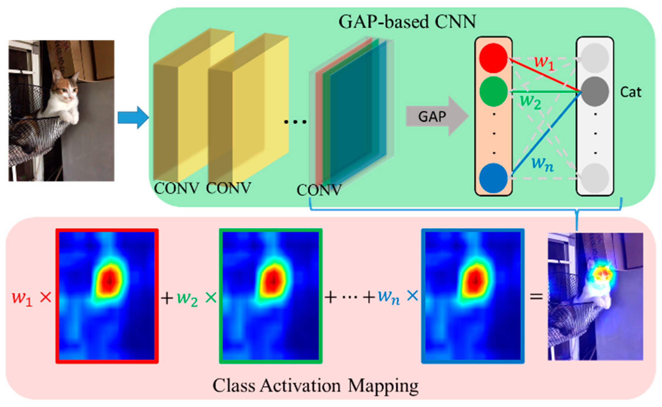
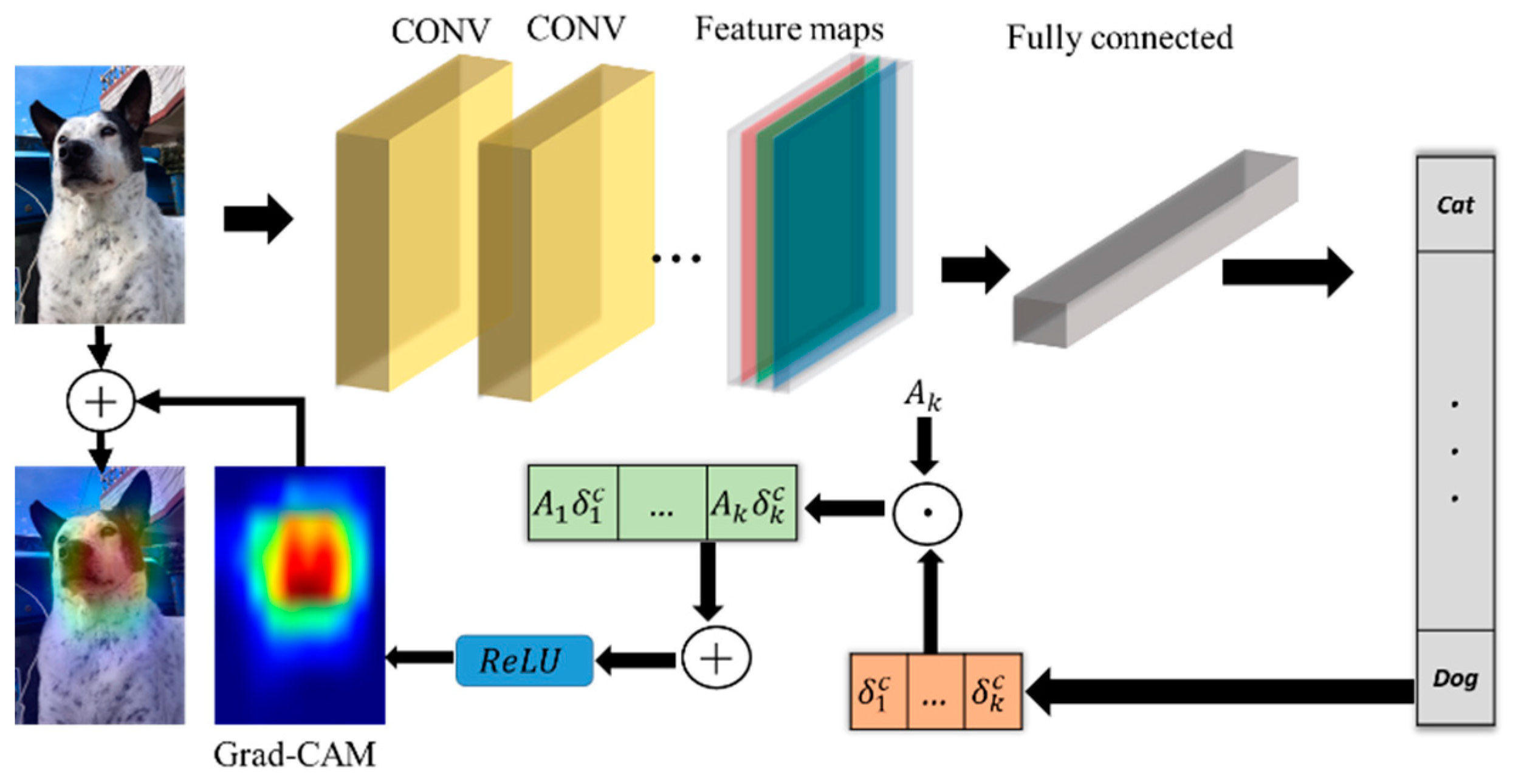
2.2. Gradient-Weighted Class Activation Mapping (Grad-CAM)

Selvaraju et al. proposed using Grad-CAM to generate a color visualization map for analyzing the region of interest of the CNN model. Grad-CAM [38] is an improvement on traditional CAM [39]. Due to the fact that CAM requires a CNN based on the global average pooling (GAP) [40] architecture, this method is difficult to apply in other CNN architectures. Different from the common pooling method, in the GAP method, which is designed to change the fully connected layer, an average function is adopted to compress each 2D feature map into a 1D vector and then classify it using the softmax function. The GAP operation is illustrated in Figure 2 and expressed in Equation (8).

$$z_c=\frac{1}{H\times W}{{\displaystyle \sum }}_{i=1}^H{{\displaystyle \sum }}_{j=1}^W{u}_{c\left(i,j\right)}$$

(8)

where $z_c$ is the cth 1D feature after the GAP operation; $H$ and $W$ are the height and width of the 2D feature map, respectively; and $u_c$ is the cth convolved feature map at position $\left(i,j\right)$. The CAM architecture is depicted in Figure 2. As displayed in Figure 2, the attention map of the model is produced from the sum of convolved feature maps and weights that are between the GAP layer and output. The detailed CAM operation is expressed in Equation (9).

$$L_{\left(x,y\right)}^c={{\displaystyle \sum }}_k{w}_k^c{A}_{k\left(x,y\right)}$$

(9)

where $L_{\left(x,y\right)}^c$ is the class activation map in category $c$, $w_k^c$ is the weight of the kth feature map, and $A_{k\left(x,y\right)}$ is the kth convolved feature map at position $\left(x,y\right)$. For overcoming the drawbacks of CAM, Grad-CAM improves the structure of the method in order to generalize various CNNs. First, the output score of each category is calculated using the following equation:

$$S_c=\frac{1}{H\times W}{{\displaystyle \sum }}_k{w}_k^c{A}_k$$

(10)

where $S_c$ is the score of the model output in category $c$; $H$ and $W$ are the height and width of the feature map, respectively; $w_k^c$ is the weight of the kth feature map in category $c$; and $A_k$ is the kth feature map. The gradient between the output score $S_c$ and the feature map $A_k$ is calculated using the following equation to acquire the category discrimination positioning map.

$${\delta }_k^c=\frac{\partial S_c}{\partial A_k}$$

(11)

$$G^c=ReLU\left({{\displaystyle \sum }}_k{\delta }_k^c{A}_k\right)$$

(12)

where ${\delta }_k^c$ denotes the weight of the kth feature map and $G^c$ is the normalized heat map of category $c$. The architecture and examples of Grad-CAM are displayed in Figure 3 and Figure 4, respectively. The benefit of Grad-CAM is that its operation is based on output results and feature maps. Therefore, the structure of the CNN does not influence the Grad-CAM operation.

The traditional CNN architecture of LeNet-5 mainly uses the convolutional layer to extract the features of the input data and apply the fully connected layer to classify the features. The convolutional layer convolved the input data and convolution kernels with a restricted region of the visual field, known as the receptive field, to automatically extract features without the need for expert experience and knowledge. However, this network architecture has the following shortcomings: (1) it is difficult for users to understand the basis of model feature extraction and (2) the use of a fully connected layer makes the network generate a large number of parameters, which requires a lot of computing time and expensive hardware costs. To improve these problems, the neuro-fuzzy network was adopted to replace the fully connected layer in the CNN network in this study. It reduces a large number of learnable parameters and improves the classification performance of the network by imitating the fuzzy logic of the human logic mechanism. In addition, by introducing the Grad-CAM method, which can generate a separate visualization image for each class, users can clearly understand the basis of network classification and provide model interpretation.

3. Problem Definition

In this section, the designed SBDS is described for bearing fault diagnosis. The proposed GC-CNFN is used to establish a predictive model for bearing fault diagnosis. This network can not only predict the current state of a bearing according to the vibration signal, but also provide gradient-weighted class activation maps of the GC-CNFN model. By merging the class activation maps and original signal images, users can understand the attention region of the vibration signal model and interpret the model. The flowchart of the proposed GC-CNFN is shown in Figure 5.

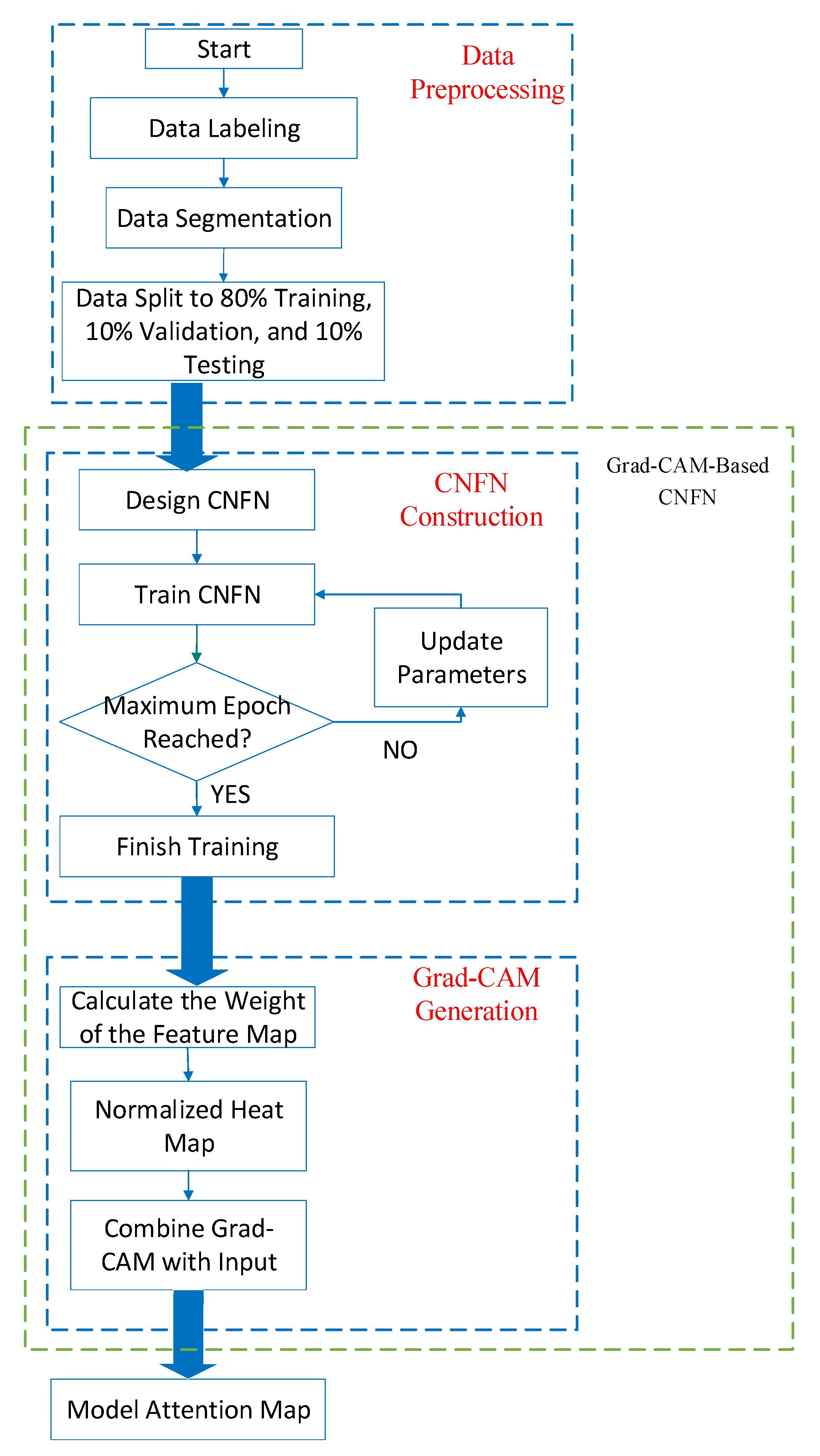
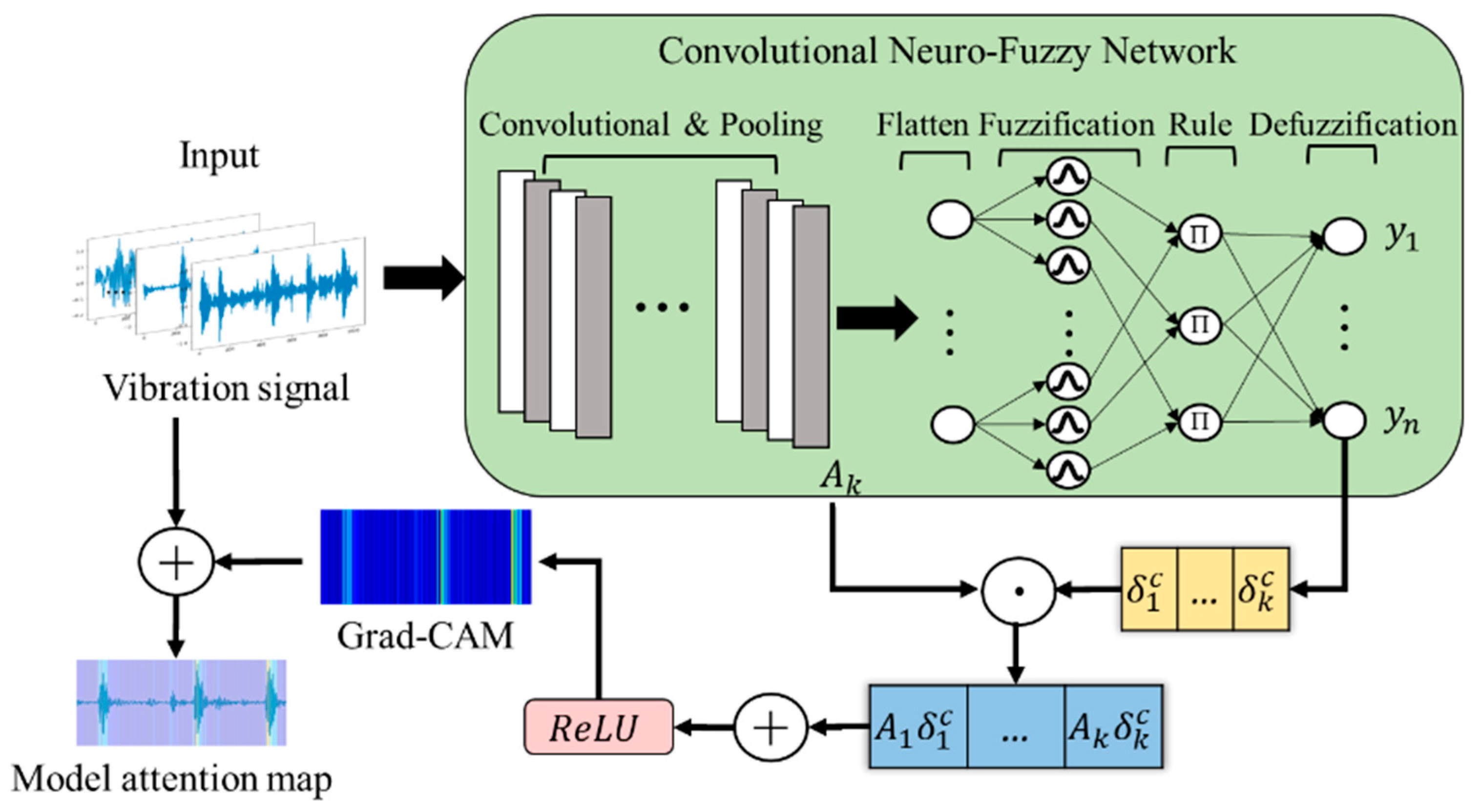
3.1. Structure of the GC-CNFN

The GC-CNFN is described in this subsection. The detailed structure of the GC-CNFN is displayed in Figure 6. As depicted in Figure 6, the GC-CNFN, which enables the prediction of bearing faults and the generation of model attention maps, combines Grad-CAM and a CNFN. To obtain a model attention map, first, the CNFN is trained to classify bearing states according to the bearing fault signal. Subsequently, Grad-CAM and a trained CNFN are used to produce the attention map of the vibration signal for analyzing the attention region of the CNFN model.

The architecture of the proposed GC-CNFN is described in detail as follows:

• Convolutional layer

In this study, the 1D convolution operation was used to extract the features of the vibration signal. The convolution operation involves performing an element-wise product operation on the input and the receptive field of the convolution kernel in a sliding window. The convolution operation is expressed as follows:

$$C_{fi}={{\displaystyle \sum }}_{v=0}^{s-1}{I}_{i+v}⨂k_{\left(f,v\right)}$$

(13)

where $C_{fi}$ denotes position i of the fth feature map after the convolution operation, $I$ represents the 1D input data, s represents the convolution kernel size, $⨂$ is the convolution operator, and $k$ is the convolution kernel at position $\left(f,v\right)$.

• Pooling layer

All the convolution feature maps are downsampled using the pooling operation. In the pooling layer, max pooling, which involves selecting the maximum value from each pooling kernel of a feature map, is adopted to reduce the number of parameters and avoid overfitting. The max pooling operation is expressed as follows:

$$P_{fj}=\underset{j\le i\le z-1}{\max }{C}_{fi}$$

(14)

where $P_{fj}$ represents the fth pooling feature map at position j, $z$ is the pooling kernel size, and $C$ is the convolution feature map.

• Flatten layer

After the feature extraction operation is completed, the flatten operation is performed to concatenate each feature map to a 1D vector. The flatten operation is expressed as follows:

$$P_{fj}\to u_i$$

(15)

$$i=f\times r+j$$

(16)

where $u_i$ is the 1D vector at position i, $P$ is the pooling feature map, and $r$ is the total number of rows in the pooling feature map.

• Fuzzification layer

In the fuzzification layer, the IF–THEN rule is used to perform the fuzzy operation. The IF–THEN rule is defined as follows:

$${\mathrm{R}}_j:\mathrm{IF}{u}_1\mathrm{is}{S}_{1j}\dots \mathrm{and}{u}_n\mathrm{is}{S}_{nj},\mathrm{THEN}{y}_j=w_j$$

where ${\mathrm{R}}_j$ denotes the fuzzy rule, $S_{ij}$ represents a fuzzy set, and $w_j$ is the zero-order Takagi–Sugeno–Kang weight. Herein, the Gaussian membership function is adopted to improve the classification result. The Gaussian membership function is expressed as follows:

$$S_{ij}=exp\left\{-\frac{{\left(u_i-m_{ij}\right)}^2}{2{\sigma }_{ij}^2}\right\}$$

(17)

where $S$ is the Gaussian membership function; $exp(·)$ is the exponential function; and $m_{ij}$ and ${\sigma }_{ij}$ are the mean and derivation of the Gaussian membership function, respectively.

• Rule layer

The fuzzy rule firing strength is obtained from the product of each membership function. The algebraic product operator is expressed as follows:

$$R_j={{\displaystyle \prod }}_{i=1}^n{S}_{ij}$$

(18)

• Defuzzification layer

The result of each rule is calculated by the defuzzification operator to obtain the crisp value. Then, the softmax function is used to acquire the output probability. The defuzzification and softmax operators are defined as follows:

$$z_i={{\displaystyle \sum }}_{j=1}^r{R}_j{w}_{ij}$$

(19)

$$y_i=softmax\left(z_i\right)$$

(20)

$$\delta \left(z_i\right)=\frac{e^{z_i}}{{{\displaystyle \sum }}_{k=1}^n{e}^{z_k}}$$

(21)

where $z$ is the crisp value obtained by the defuzzifier, $R$ is the firing strength of the fuzzy rule, $w$ is the weight, $y_i$ is the output probability of the ith category, and $\delta (·)$ is the softmax activation function that performs exponential normalization for normalizing the output value between 0 and 1.

3.2. Parameter Learning Phase

In the learning process, the back-propagation algorithm is used to update the parameters of the CNFN. By minimizing the loss function, the gradient of each neuron can be computed. In this subsection, the cross-entropy loss function is used to complete a multiclass classification task. The cross-entropy loss function $L$ is defined as follows:

$$L=-{{\displaystyle \sum }}_i{t}_i\log \left(y_i\right)$$

(22)

where $t_i$ is the real category and $y_i$ is the model prediction result. The trainable parameters in the CNFN include $w_{ij}, m_{ij}, {\sigma }_{ij},$ and $k_{f,v}$. These parameters are adjusted by the back-propagation learning algorithm to minimize the loss function. The updated parameters are defined as follows:

$$w_{ij}\left(t+1\right)=w_{ij}\left(t\right)-{\eta }_w\Delta w_{ij}$$

(23)

where

$$\Delta w_{ij}=\frac{\partial L}{\partial w_{ij}}=\frac{\partial L}{\partial \widehat{y}}\frac{\partial \widehat{y}}{\partial w_{ij}}$$

$$m_{ij}\left(t+1\right)=m_{ij}\left(t\right)-{\eta }_m\Delta m_{ij}$$

(24)

where

$$\Delta m_{ij}=\frac{\partial L}{\partial m_{ij}}=\frac{\partial L}{\partial s_{ij}}\frac{\partial s_{ij}}{\partial m_{ij}}$$

$${\sigma }_{ij}\left(t+1\right)={\sigma }_{ij}\left(t\right)-{\eta }_{\sigma }\Delta {\sigma }_{ij}$$

(25)

where

$$\Delta {\sigma }_{ij}=\frac{\partial L}{\partial {\sigma }_{ij}}=\frac{\partial L}{\partial s_{ij}}\frac{\partial s_{ij}}{\partial {\sigma }_{ij}}$$

$$k_{f,v}\left(t+1\right)=k_{f,v}\left(t\right)-{\eta }_k\Delta k_{f,v}$$

(26)

where

$$\Delta k_{f,v}=\frac{\partial L}{\partial k_{f,v}}=\frac{\partial L}{\partial C_{fi}}\frac{\partial C_{fi}}{\partial k_{f,v}}$$

where ${\eta }_w, {\eta }_m, {\eta }_{\sigma }$, and ${\eta }_k$ are the learning rates of the weight, mean and derivation of the Gaussian membership function, and convolution kernel, respectively. After network construction is completed, the CNFN is trained using vibration signals and applied in fault classification tasks. The trained CNFN and Grad-CAM methods are used to generate the attention map of the model, facilitating the analysis of the vibration signal region that the model focuses on.

4. Experimental Results

In this section, the performance of the GC-CNFN is described. First, the CWRU bearing dataset [41] was used to train the proposed GC-CNFN and verify its efficiency. The input of the GC-CNFN was the raw vibration signal, and its output was the current state of the bearing. Next, the CNFN attention map was generated through Grad-CAM. By merging the attention map and raw vibration signal to create a classification visualization, the classification of bearing faults could be better understood. The procedure and results of the conducted experiment are described in detail in the following text.

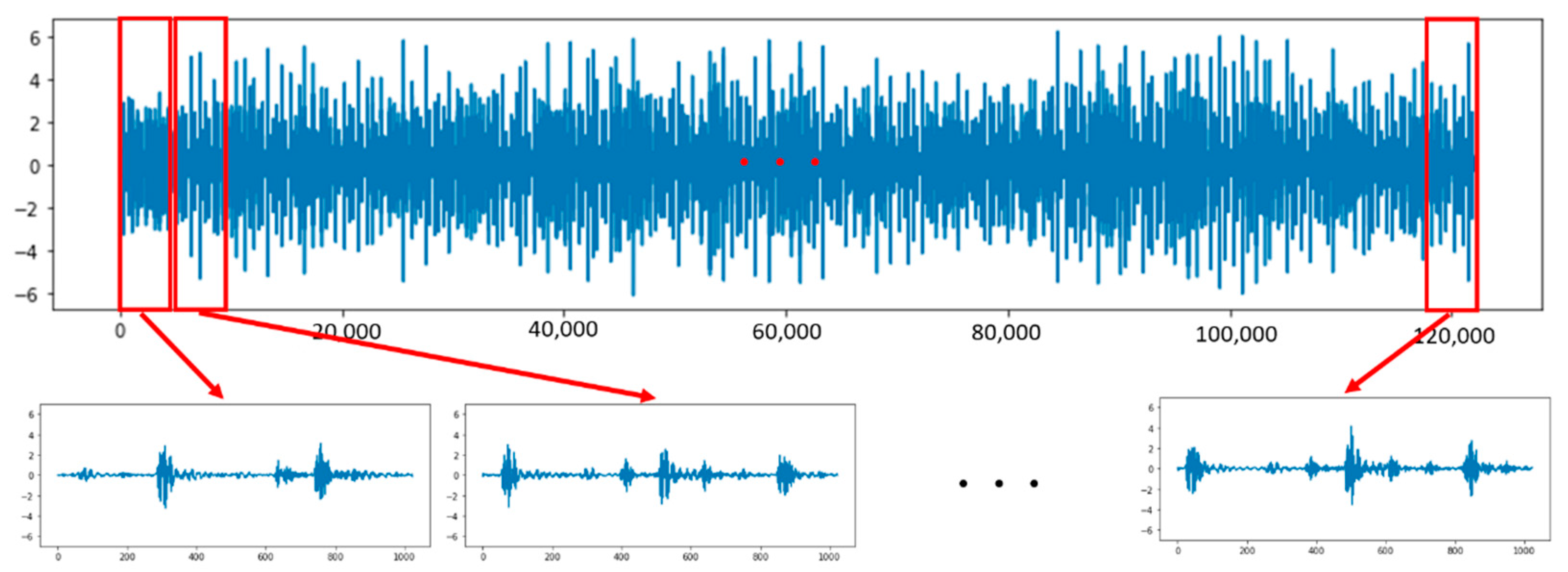
4.1. Data Preprocessing

The CWRU bearing dataset was adopted to train the GC-CNFN model. The CWRU bearing dataset includes normal and faulty bearing vibration signals, which were collected through electrical discharge machining (EDM). The machine used for EDM has an electric motor, a drive-end bearing, a torque transducer, and a dynamometer, as displayed in Figure 7a. The bearing database covers four states: normal, ball fault, inner race fault, and outer race fault. The CWRU database includes vibration signals that were collected under sampling frequencies of 12 kHz and 48 kHz and motor loads of 0, 1, 2, and 3 horsepower. The diameters of the normal, ball fault, inner race fault, and outer race fault states are 0, 0.007, 0.014, 0.021, and 0.028 inches, respectively. The corresponding motor speeds of the four loads are 1797, 1772, 1750, and 1730 rpm, respectively. Considering the fault location corresponding to the load zone, the outer race faults are divided into three categories: centered, orthogonal, and opposite outer race faults. Centered outer race faults are located at 6 o’clock (@6), orthogonal outer race faults are located at 3 o’clock (@3), and opposite outer race faults are located at 12 o’clock (@12). The structure of the rolling bearing is shown in Figure 7b. As depicted in Figure 7b, the rolling bearing is generally composed of an inner ring, an outer ring, and steel balls. In the experiment, we focused on the data corresponding to a sampling frequency of 12 kHz and did not consider motor load and motor speed. Thus, 16 bearing conditions were used to establish a bearing fault diagnosis system. For example, all inner race faults that had a diameter of 0.007 inches, irrespective of the motor load and motor speed, were assumed to be in one category. The health conditions corresponding to different bearing vibration signals are presented in

Table 1. Status conditions corresponding to different bearing vibration signals.

Fault Diameter	Motor Load	Motor Speed	Normal	Inner Race	Ball	Outer Race (Fault Position)
						@6	@3	@12
0	0	1797	Normal	—	—	—	—	—
	1	1772
	2	1750
	3	1730
0.007	0	1797	—	IR_07	B_07	OR@6_07	OR@3_07	OR@12_07
	1	1772
	2	1750
	3	1730
0.014	0	1797	—	IR_14	B_14	OR@6_14	OR@3_14	—
	1	1772
	2	1750
	3	1730
0.021	0	1797	—	IR_21	B_21	OR@6_21	—	OR@12_21
	1	1772
	2	1750
	3	1730
0.028	0	1797	—	IR_28	B_28	—	—	—
	1	1772
	2	1750
	3	1730

, where the symbol “—” indicates that data were unavailable. The 16 status conditions were labeled as Normal, IR_07, IR_14, IR_21, IR_28, B_07, B_014, B_21, B_28, OR@6_07, OR@6_14, OR@6_21, OR@3_07, OR@3_14, OR@12_07, and OR@12_21.

To identify the status of a bearing, the 12-kHz CWRU dataset was preprocessed to establish a bearing fault diagnosis model. The total number of 12 kHz driver fault records was 64. Each health condition had four vibration signal records. Each record was split into several nonoverlapping fragment samples, each of which contained 1024 points. A processed data segment is illustrated in Figure 8. The number of samples in each fault category is listed in

Table 2. Number of samples in each fault category.

Fault Diameter	Normal	Inner Race	Ball	Outer Race (Fault Position)
				@6	@3	@12
0	1657	—	—	—	—	—
0.007	—	476	473	475	474	476
0.014	—	472	475	474	475	—
0.021	—	474	475	476	—	474
0.028	—	471	471	—	—	—

. As presented in Table 2, the normal, ball fault, inner race fault, and outer race fault states contained 1657, 1893, 1894, and 3324 samples, respectively. These processed data were used to train the CNN model for bearing fault diagnosis.

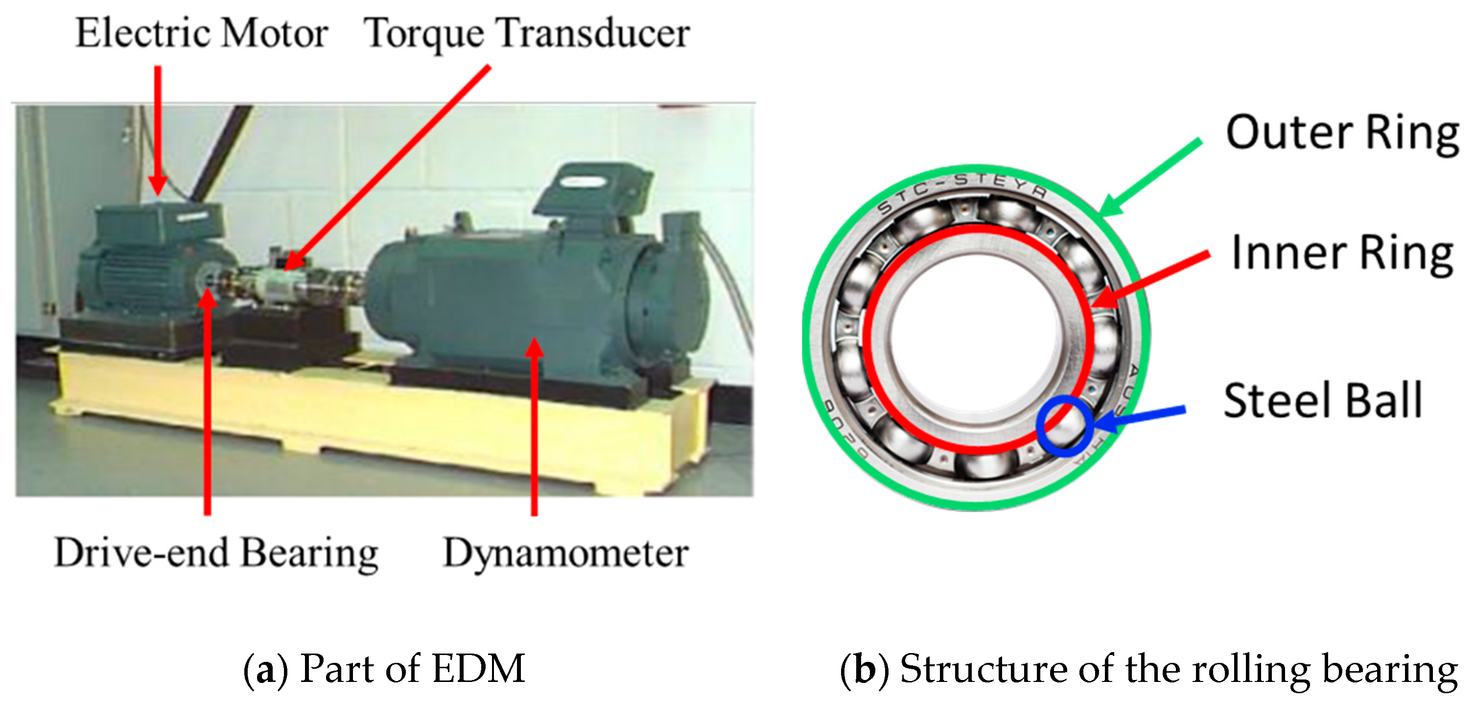
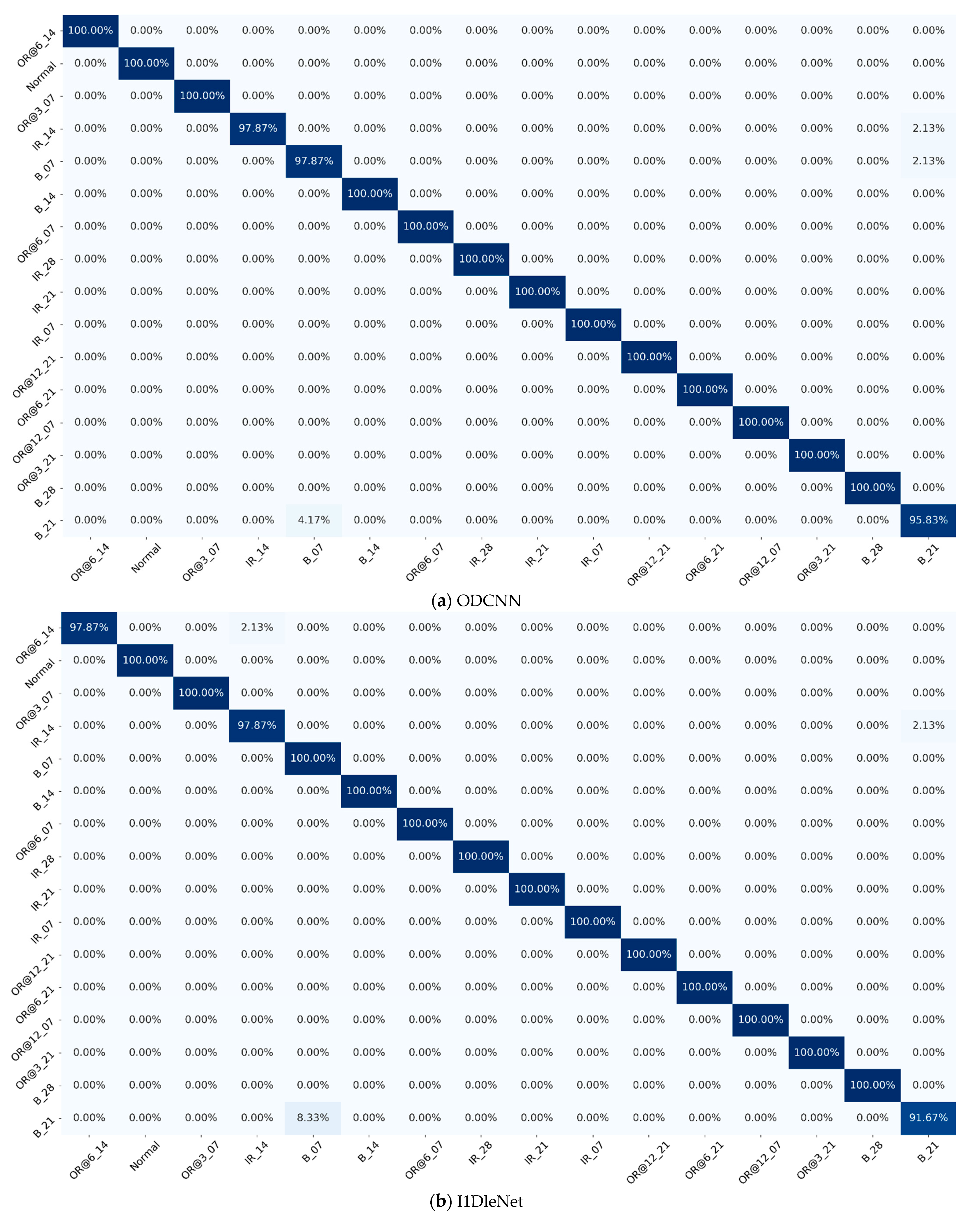
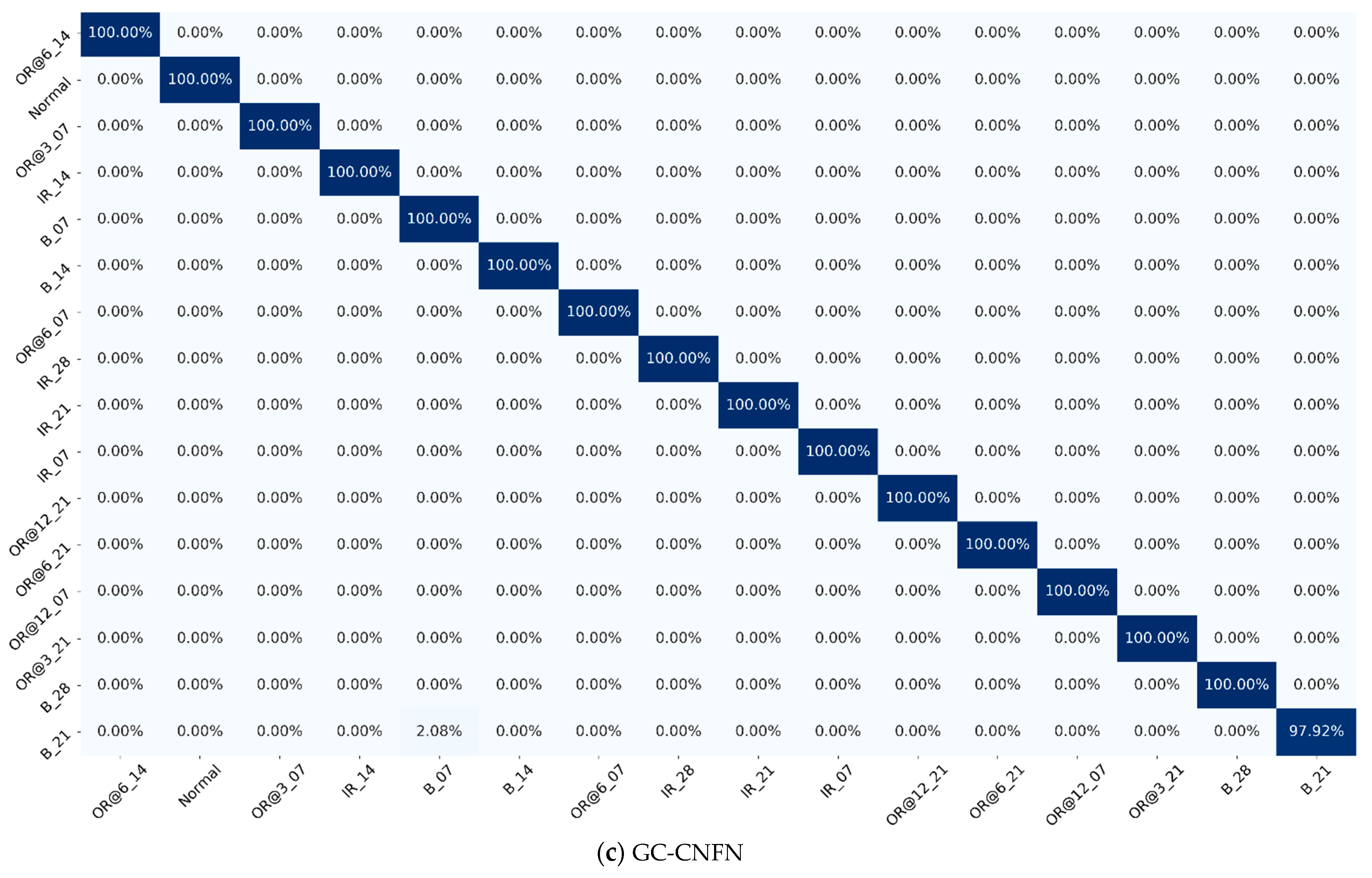
4.2. Bearing Fault Diagnosis and Evaluation for CWRU Dataset

This subsection describes the results of bearing fault diagnosis when using the proposed GC-CNFN. The detailed architecture and parameters of the GC-CNFN are presented in

Table 3. Architecture of the GC-CNFN.

Layer	Parameter
Input	1024 $\times$ 1
Conv1D (size, channel)	32 $\times$ 1, 5
Conv1D (size, channel)	16 $\times$ 1, 3
Max-pooling (size, stride)	10 $\times$ 1, 1
Fuzzy (rule)	32
Defuzzifier (Output)	16

. As presented in Table 3, the GC-CNFN contains two convolutional layers, one max pooling layer, one fuzzy layer, and one defuzzification layer. To obtain the attention map of the GC-CNFN model, the padding operation was used for maintaining the dimensions of the convolutional feature map in the first layer. The first and second convolution layers contained kernels with sizes of 32 × 1 and 16 × 1, respectively, and the channel sizes were 5 and 3, respectively. The size of the max pooling kernel was 10 × 1. The number of fuzzy rules was set as 32. The output was one of the 16 bearing fault conditions. A total of 8768 vibration signals were used to train the GC-CNFN. The vibration signal data were split as follows: 80% for training, 10% for validation, and 10% for testing; thus, the total numbers of training, validation, and testing samples were 7014, 877, and 877, respectively.

To evaluate the stability and generalization performance of the GC-CNFN effectively, 10 training processes were adopted in the experiment. The k-fold cross-validation method [40] was also used to verify the model efficiency for different subsets. The performance of the GC-CNFN was compared with that of the ODCNN and improved 1D LeNet-5 (I1DLeNet). The detailed network structures of the ODCNN and I1DLeNet are presented in

Table 4. ODCNN and I1DLeNet structures.

	Model	ODCNN	I1DLeNet
Layer
Convolutional 1 (size, channel)		10 × 1, 50	6 × 64, 50
Pooling 1 (size, stride, mode)		2 × 1, A	8 × 1, 8, M
Convolutional 2 (size, channel)		20 $\times$ 50, 5	16 × 1, 16
Pooling 2 (size, stride, mode)		2 × 1, A	2 × 1, 1, M
Convolutional 3 (size, channel)		—	32 × 1, 8
Pooling 3 (size, stride, mode)		—	2 × 1, 1, M
Convolutional 4 (size, channel)		—	32 × 1, 4
Pooling 4 (size, stride, mode)		—	2 × 1, 1, M
Fully connected (neuron)		200	120
Fully connected (neuron)		200	84
Output		16	16

. The ODCNN contains two sets of convolution, pooling, and fully connected layers. I1DLeNet contains four sets of convolution and pooling layers as well as two sets of fully connected layers. For the pooling layer, mode A and mode B indicate average pooling and max pooling, respectively.

The implementation of GC-CNFN was done by using Tensorflow 1.14, Keras 2.3.0, and Python 2.7. Due to the fact that obtaining sufficient GPU computing resources in a factory is difficult, a 3.00-GHz Intel Core i5-8500 central processing unit with six cores computer was adopted in the experiment to evaluate the computing performance of the three compared models. A total of 50 epochs were used to train each model. The results obtained for each model after ten training processes are presented in

Table 5. Training results of each model.

	Model	ODCNN [28]	I1DLeNet [29]	GC-CNFN
Evaluation Item
Training	Best accuracy	0.9962	0.9949	0.9975
	Worst accuracy	0.9922	0.9913	0.9924
	Average accuracy	0.9947	0.9835	0.9955
	Standard deviation	0.0028	0.0040	0.0019
Total parameters		1,078,146	375,122	20,248
Average training time (s)		217.6	141.5	117.7
Testing accuracy		0.9931	0.9874	0.9988

. The evaluation variables in the experiment included accuracy, standard deviation (SD), total number of parameters, and average training time.

As presented in Table 5, the ODCNN and GC-CNFN had the highest accuracy rates of 99.62% and 99.75%, respectively. The proposed GC-CNFN had the highest average accuracy and lowest SD. The aforementioned results indicate that the proposed method is relatively stable for bearing fault diagnosis. The number of parameters and calculation times were also determined to evaluate the computation efficiency of each model. The ODCNN had the largest number of parameters (up to 1.07 million) because it used a large number of neurons in the fully connected layer. The I1DLeNet used fewer neurons in the fully connected layer and therefore required 2.87 times fewer parameters and exhibited a computation time that was 1.45 times shorter than ODCNN. In the proposed GC-CNFN, the neuro-fuzzy network replaces the traditional fully connected layer, which considerably reduces the number of parameters and the required computation resources. Compared with the ODCNN and I1DLeNet, the GC-CNFN required 53.2 and 18.5 times fewer parameters, respectively, and computation times that were 1.88 and 1.28 times shorter, respectively. The confusion matrices of each model are shown in Figure 9. The ODCNN classified a small number of ball faults with a diameter of 0.021 inches (B_21) as ball faults with a diameter of 0.007 inches (B_07) and inner race faults with a diameter of 0.017 inches (IR_14). The I1DLeNet model classified some ball faults with a diameter of 0.021 inches (B_21) as ball faults with a diameter of 0.007 inches (B_07) and inner race faults with a diameter of 0.017 inches (IR_14), respectively. A small number of outer race faults, which were located at 6 o’clock with a diameter of 0.14 inches (OR@6_14) were also classified as inner race faults with a diameter of 0.017 inches (IR_14). The proposed GC-CNFN misclassified partial ball faults with a diameter of 0.021 inches (B_21) as ball faults with a diameter of 0.007 inches (B_07). This result indicates that the characteristics of B_07 and B_21 were similar, which resulted in model classification errors.

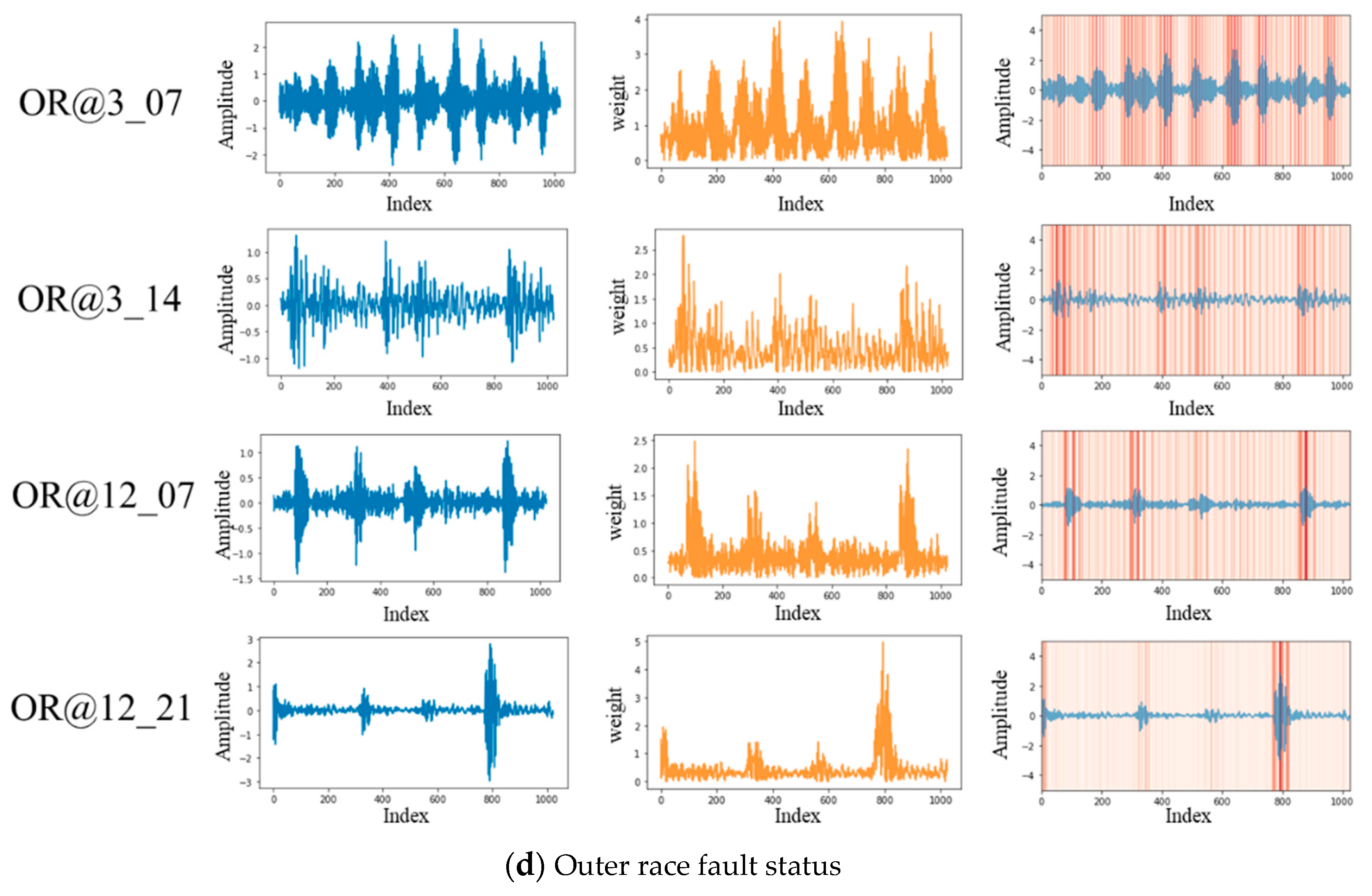
4.3. Model Attention Map for Vibration Signals

After the training process, the GC-CNFN was used to generate a model attention map to analyze the region, in which the model focused on vibration signals. First, the activation map of the model was obtained using the convolution kernel. Then, the vibration signal was combined with the activation map to obtain a model attention map. The model attention maps of different types of bearing faults are displayed in Figure 10. Figure 10a illustrates the vibration signal in the normal state. The amplitude of the vibration signal in the normal state was between 0.2 and −0.2, which was smaller than the amplitude of other fault states. The activation map focused on the vibration signal with larger amplitudes, which indicated that the GC-CNFN had learned the characteristics of the vibration signal in the normal state. The vibration signals of the four types of inner ring fault states contained many waves with different amplitudes, as displayed in Figure 10b. An analysis of the model attention maps indicated that the GC-CNFN principally focused on large-amplitude waveforms. As depicted in Figure 10c, the B_07 and B21 ball failure states were highly similar; therefore, the GC-CNFN was prone to misclassify these failure states. The vibration signal amplitude of B_28 was larger than those of other fault signals, which were between 7.5 and −7.5. Figure 10d illustrates the vibration signals of outer race faults in three failure positions. Different fault states exhibited different waveforms. The model attention maps indicate that the proposed GC-CNFN can automatically extract feature information on different fault signals. Thus, the GC-CNFN achieves high accuracy in fault classification.

In the experimental results (Table 5), we found that the parameters of ODCNN and I1DLeNet using the fully connected layer were surprisingly large, exceeding 1 million and 300,000 respectively. On the contrary, the proposed GC-CNFN adopted the neuro-fuzzy network to replace the fully connected layer, which not only greatly reduced the number of network parameters, but also increased the classification accuracy. This indicates that the neural-fuzzy network, which combines the human reasoning mechanism of fuzzy logic and nonlinear mapping of NN, has a greater superiority to the fully connected layer. From the model attention map (Figure 10), we observed that some bearing defects were classified incorrectly due to similar vibration signal characteristics, such as B_07 and B_21. The three network architectures (ODCNN, I1DLeNet, and GC-CNFN) in the experiment encountered this problem. In future studies, we will consider introducing the attention mechanism to improve the problem of bearing fault misclassifications due to similar fault signals.

5. Conclusions

In this study, an SBDS was developed for diagnosing bearing faults of tool machines. Considering that traditional modeling methods rely on experts for tedious manual feature extraction, the SBDS uses the designed GC-CNFN, which can automatically perform feature extraction from the original raw vibration signal to establish a predictive model for bearing fault diagnosis. The proposed GC-CNFN applies the neuro-fuzzy network to replace the fully connected layer in order to reduce the number of network parameters and improve the classification accuracy. Simultaneously, the proposed GC-CNFN also introduces the Grad-CAM method to generate the model attention maps that provide users with the ability to understand the basis of model classification of bearing faults. The experimental results indicated that the GC-CNFN required fewer parameters (20K), had a shorter average calculation time (117.7s), and had a higher prediction accuracy (99.88%) than ODCNN and I1DLeNet-5 models. Inevitably, the proposed GC-CNFN model has limitations. For example, the number of parameters and fuzzy rules in the GC-CNFN model depends on user experience or trial and error. In future works, the automatic selection of parameters and fuzzy rules in the GC-CNFN model will be considered to improve the model’s effectiveness. Simultaneously, different bearing databases will also be considered to verify the stability and robustness of the classification model. Finally, in order to achieve high-speed operation in real-time applications, the GC-CNFN model will also be implemented on a field programmable gate array.

References

1. On Recommended Interval of Updating Induction Motors; JEMA: Tokyo, Japan, 2000. (In Japanese)
2. Motor Reliability Working Group. Report of large motor reliability survey of industrial and commercial installations, Part, I. IEEE Trans. Ind. Appl. 1985, IA-21, 853–864. [Google Scholar] [CrossRef]
3. Motor Reliability Working Group. Report of large motor reliability survey of industrial and commercial installations, Part II. IEEE Trans. Ind. Appl. 1985, IA-21, 865–872. [Google Scholar] [CrossRef]
4. Motor Reliability Working Group. Report of large motor reliability survey of industrial and commercial installations: Part 3. IEEE Trans. Ind. Appl. 1987, IA-23, 153–158. [Google Scholar] [CrossRef]
5. Akyurt, I.; Kuvvetli, Y.; Deveci, M. Enterprise Resource Planning in The Age of Industry 4.0 A General Overview; CRC Press: Boca Raton, FL, USA, 2020; pp. 178–185. [Google Scholar]
6. Afshari, N.; Loparo, K.A. A Model-Based Technique for the Fault Detection of Rolling Element Bearings Using Detection Filter Design and Sliding Mode Technique. In Proceedings of the 37th IEEE Conference on Decision and Control, Tampa, FL, USA, 18 December 1998. [Google Scholar]
7. White, J.; Speyer, J. Detection filter design: Spectral theory and algorithms. IEEE Trans. Autom. Control. 1987, 32, 593–603. [Google Scholar] [CrossRef]
8. Slotine, J.E.; Hedrick, J.K.; Misawa, E.A. On Sliding Observers for Nonlinear Systems. In Proceedings of the 1986 American Control Conference, Seattle, WA, USA, 18–20 June 1986. [Google Scholar]
9. Adams, M.L. Analysis of Rolling Element Bearing Faults in Rotating Machinery: Experiments, Modeling, Fault Detection and Diagnosis; Case Western Reserve University: Cleveland, OH, USA, 2001. [Google Scholar]
10. Forst, W.; Hoffmann, D. Optimization—Theory and Practice; Springer: New York, NY, USA, 2010. [Google Scholar]
11. Jalan, A.K.; Mohanty, A.R. Model based fault diagnosis of a rotor–bearing system for misalignment and unbalance under steady-state condition. J. Sound Vib. 2009, 327, 604–622. [Google Scholar] [CrossRef]
12. Simani, S.; Fantuzzi, C.; Patton, R. Model-Based Fault Diagnosis in Dynamic Systems Using Identification Techniques; Springer: London, UK, 2003. [Google Scholar]
13. Nikolaou, N.G.; Antoniadis, I.A. Rolling element bearing fault diagnosis using wavelet packets. NDT E Int. 2002, 35, 197–205. [Google Scholar] [CrossRef]
14. Cocconcelli, M.; Zimroz, R.; Rubini, R.; Bartelmus, W. STFT Based Approach for Ball Bearing Fault Detection in a Varying Speed Motor. In Condition Monitoring of Machinery in Non-Stationary Operations; Fakhfakh, T., Bartelmus, W., Chaari, F., Zimroz, R., Haddar, M., Eds.; Springer: Berlin/Heidelberg, Germany, 2012; pp. 41–50. [Google Scholar]
15. Van, M.; Kang, H.-J.; Shin, K.-S. Rolling element bearing fault diagnosis based on non-local means de-noising and empirical mode decomposition. IET Sci. Meas. Technol. 2014, 8, 571–578. [Google Scholar] [CrossRef]
16. Ville, D.V.D.; Kocher, M. Sure-based non-local means. IEEE Signal Process. Lett. 2009, 16, 973–976. [Google Scholar] [CrossRef] [Green Version]
17. Tracey, B.H.; Miller, E.L. Nonlocal means denoising of ECG signals. IEEE Trans. Biomed. Eng. 2012, 59, 2383–2386. [Google Scholar] [CrossRef]
18. Junsheng, C.; Dejie, Y.; Yu, Y. A fault diagnosis approach for roller bearings based on EMD method and AR model. Mech. Syst. Signal Process. 2006, 20, 350–362. [Google Scholar] [CrossRef]
19. Fu, S.; Liu, K.; Xu, Y.G.; Liu, Y. Rolling Bearing Diagnosing Method Based on Time Domain Analysis and Adaptive Fuzzy C-Means Clustering. Shock. Vib. 2016, 2016, 1–8. [Google Scholar] [CrossRef] [Green Version]
20. Yuwono, M.; Qin, Y.; Zhou, J.; Guo, Y.; Celler, B.G.; Su, S.W. Automatic bearing fault diagnosis using particle swarm clustering and Hidden Markov Model. Eng. Appl. Artif. Intell. 2016, 47, 88–100. [Google Scholar] [CrossRef]
21. Ben Ali, J.; Fnaiech, N.; Saidi, L.; Chebel-Morello, B.; Fnaiech, F. Application of empirical mode decomposition and artificial neural network for automatic bearing fault diagnosis based on vibration signals. Appl. Acoust. 2015, 89, 16–27. [Google Scholar] [CrossRef]
22. Ertunc, H.M.; Ocak, H.; Aliustaoglu, C. ANN- and ANFIS-based multi-staged decision algorithm for the detection and diagnosis of bearing faults. Neural Comput. Appl. 2013, 22, 435–446. [Google Scholar] [CrossRef]
23. Jang, J.R. ANFIS: Adaptive-network-based fuzzy inference system. IEEE Trans. Syst. Man Cybern. 1993, 23, 665–685. [Google Scholar] [CrossRef]
24. Deveci, M.; Pekaslan, D.; Canıtez, F. The assessment of smart city projects using zSlice type-2 fuzzy sets based interval agreement method. Sustain. Cities Soc. 2020, 53, 101889. [Google Scholar] [CrossRef]
25. Zhang, W.; Peng, G.; Li, C.; Chen, Y.; Zhang, Z. A new deep learning model for fault diagnosis with good anti-noise and domain adaptation ability on raw vibration signals. Sensors 2017, 17, 425. [Google Scholar] [CrossRef]
26. Wen, L.; Li, X.; Gao, L.; Zhang, Y. A new convolutional neural network-based data-driven fault diagnosis method. IEEE Trans. Ind. Electron. 2018, 65, 5990–5998. [Google Scholar] [CrossRef]
27. Tax, D.; Ypma, A.; Duin, R. Pump Failure Detection Using Support Vector Data Descriptions; Springer: Heidelberg/Berlin, Germany, 1999; Volume 1642, pp. 415–426. [Google Scholar]
28. Lei, Y.; Jia, F.; Lin, J.; Xing, S.; Ding, S.X. An intelligent fault diagnosis method using unsupervised feature learning towards mechanical big data. IEEE Trans. Ind. Electron. 2016, 63, 3137–3147. [Google Scholar] [CrossRef]
29. Shao, H.; Jiang, H.; Zhang, X.; Niu, M. Rolling bearing fault diagnosis using an optimization deep belief network. Meas. Sci. Technol. 2015, 26, 115002. [Google Scholar] [CrossRef]
30. Xie, S.; Ren, G.; Zhu, J. Application of a new one-dimensional deep convolutional neural network for intelligent fault diagnosis of rolling bearings. Sci. Prog. 2020, 103, 0036850420951394. [Google Scholar] [CrossRef]
31. Wan, L.; Chen, Y.; Li, H.; Li, C. Rolling-element bearing fault diagnosis using improved lenet-5 network. Sensors 2020, 20, 1693. [Google Scholar] [CrossRef] [Green Version]
32. LeCun, Y.; Bengio, Y. Convolutional networks for images, speech, and time series. In The Handbook of Brain Theory and Neural Networks; MIT Press: Cambridge, MA, USA, 1998; pp. 255–258. [Google Scholar]
33. Dolz, J.; Desrosiers, C.; Ben Ayed, I. 3D fully convolutional networks for subcortical segmentation in MRI: A large-scale study. NeuroImage 2018, 170, 456–470. [Google Scholar] [CrossRef] [Green Version]
34. Ji, S.; Xu, W.; Yang, M.; Yu, K. 3D convolutional neural networks for human action recognition. IEEE Trans. Pattern Anal. Mach. Intell. 2013, 35, 221–231. [Google Scholar] [CrossRef] [Green Version]
35. Scherer, D.; Müller, A.; Behnke, S. Evaluation of Pooling Operations in Convolutional Architectures for Object Recognition; Springer: Heidelberg/Berlin, Germany, 2010; pp. 92–101. [Google Scholar]
36. Yu, D.; Wang, H.; Chen, P.; Wei, Z. Mixed Pooling for Convolutional Neural Networks; Springer: Cham, Swizerland, 2014; pp. 364–375. [Google Scholar]
37. Thiyagalingam, J.; Beckmann, O.; Kelly, P.H.J. An Exhaustive Evaluation of Row-Major, Column-Major and Morton Layouts for Large Two-Dimensional Arrays. In Performance Engineering: 19th Annual UK Performance Engineering Workshop; Jarvis, S.A., Ed.; University of Warwick: Coventry, UK, 2003; pp. 340–351. [Google Scholar]
38. Selvaraju, R.R.; Cogswell, M.; Das, A.; Vedantam, R.; Parikh, D.; Batra, D. Grad-CAM: Visual Explanations from Deep Networks via Gradient-Based Localization. In Proceedings of the 2017 IEEE International Conference on Computer Vision (ICCV), Venice, Italy, 22–29 October 2017; pp. 618–626. [Google Scholar]
39. Zhou, B.; Khosla, A.; Lapedriza, A.; Oliva, A.; Torralba, A. Learning Deep Features for Discriminative Localization. In Proceedings of the 2016 IEEE Conference on Computer Vision and Pattern Recognition (CVPR), Las Vegas, NV, USA, 27–30 June 2016; pp. 2921–2929. [Google Scholar]
40. Lin, M.; Chen, Q.; Yan, S. Network in Network. arXiv 2013, arXiv:1312.4400. [Google Scholar]
41. Smith, W.A.; Randall, R.B. Rolling element bearing diagnostics using the case western reserve university data: A benchmark study. Mech. Syst. Sig. Process. 2015, 64–65, 100–131. [Google Scholar] [CrossRef]
Figure 1. Architecture of LeNet-5.
Mathematics 09 01502 g001
Figure 2. CAM architecture.
Mathematics 09 01502 g002
Figure 3. Grad-CAM architecture.
Mathematics 09 01502 g003
Figure 4. Examples of Grad-CAM.
Mathematics 09 01502 g004
Figure 5. Flowchart of the GC-CNFN.
Mathematics 09 01502 g005
Figure 6. Structure of the GC-CNFN.
Mathematics 09 01502 g006
Figure 7. EDM and rolling bearing.
Mathematics 09 01502 g007
Figure 8. Processed data segment.
Mathematics 09 01502 g008
Figure 9. Confusion matrices of each model.
Mathematics 09 01502 g009aMathematics 09 01502 g009b
Figure 10. Model attention maps for different types of bearing faults.
Mathematics 09 01502 g010aMathematics 09 01502 g010bMathematics 09 01502 g010c