A Fuzzy Seasonal Long Short-Term Memory Network for Wind Power Forecasting

Abstract

To protect the environment and achieve the Sustainable Development Goals (SDGs), reducing greenhouse gas emissions has been actively promoted by global governments. Thus, clean energy, such as wind power, has become a very important topic among global governments. However, accurately forecasting wind power output is not a straightforward task. The present study attempts to develop a fuzzy seasonal long short-term memory network (FSLSTM) that includes the fuzzy decomposition method and long short-term memory network (LSTM) to forecast a monthly wind power output dataset. LSTM technology has been successfully applied to forecasting problems, especially time series problems. This study first adopts the fuzzy seasonal index into the fuzzy LSTM model, which effectively extends the traditional LSTM technology. The FSLSTM, LSTM, autoregressive integrated moving average (ARIMA), generalized regression neural network (GRNN), back propagation neural network (BPNN), least square support vector regression (LSSVR), and seasonal autoregressive integrated moving average (SARIMA) models are then used to forecast monthly wind power output datasets in Taiwan. The empirical results indicate that FSLSTM can obtain better performance in terms of forecasting accuracy than the other methods. Therefore, FSLSTM can efficiently provide credible prediction values for Taiwan’s wind power output datasets.

1. Introduction

Wind power generation is replacing power generation via extensive gas-flow and uses wind to drive wind turbines. In 2000, to protect the environment, the Taiwanese government actively promoted the use of clean energy to reduce the greenhouse gas emissions generated by traditional power generation methods such as thermal power generation. The Taiwanese government’s expectations for wind power generation are very high. The government has developed an offshore wind power facility, the main goal of which is to generate enough electricity so that renewable energy can replace nuclear power generation. The vision of the Taiwanese government is to build a strong support industry by manufacturing the necessary wind turbine components, towers, and underwater cables for coastal engineering; by building underwater foundation pile; and by installing generators several miles offshore. According to statistics from the International Energy Agency, offshore wind power currently accounts for only 0.3% of global power generation, but experts have noted that wind power generation is expected to rapidly grow in the next 20 years, representing a business opportunity of up to one trillion US dollars. Therefore, the accuracy of wind power forecasting is a very important issue that could help governments to engage in effective policy planning. In recent years, many studies have investigated wind speed and power forecasting and adopted various prediction models to improve wind power generation forecasting. Lu et al. [1,2] used the Takagi–Sugeno fuzzy model to predict wind speed and power. Yu et al. [3] developed hybrid models that combine the wavelet transform (WT) with the support vector machine (SVM), gated recurrent units network (GRU), standard recurrent neural network (RNN), and LSTM models for wind-speed forecasting. Using the WT can decompose the original wind time series into several subseries with better behavior and greater predictability. The results indicated that the hybrid models WT-RNN-SVM, WT-LSTM-SVM, and WT-GRU-SVM obtained the best performance. Zjavka and Mišák [4] noted that wind output power forecasting entails chaotic large-scale patterns and has a high correlation with atmospheric circulation processes. The authors adopted the polynomial decomposition of the general differential equation, which represents the elementary Laplace transformations of a searched function, to predict the daily wind power. The results showed that their method can obtain lower casual errors due to using the decomposition method. Liu et al. [5] used combined wavelet packet decomposition with a convolutional neural network and convolutional long short-term memory network to forecast one-day wind speed. In the one-day wind speed time series, the model was able to obtain robust and effective performance. Toubeau et al. [6] adopted the LSTM to efficiently capture the complex temporal dynamics needed for wind power prediction.

When the RNN is applied to long-term dependence, the processing unit will continue to add and calculate the previously memorized information, causing the neural network to explode or disappear and eventually leading the network to collapse. Recurrent neural networks are weak in terms of learning long-term dependence [7]. 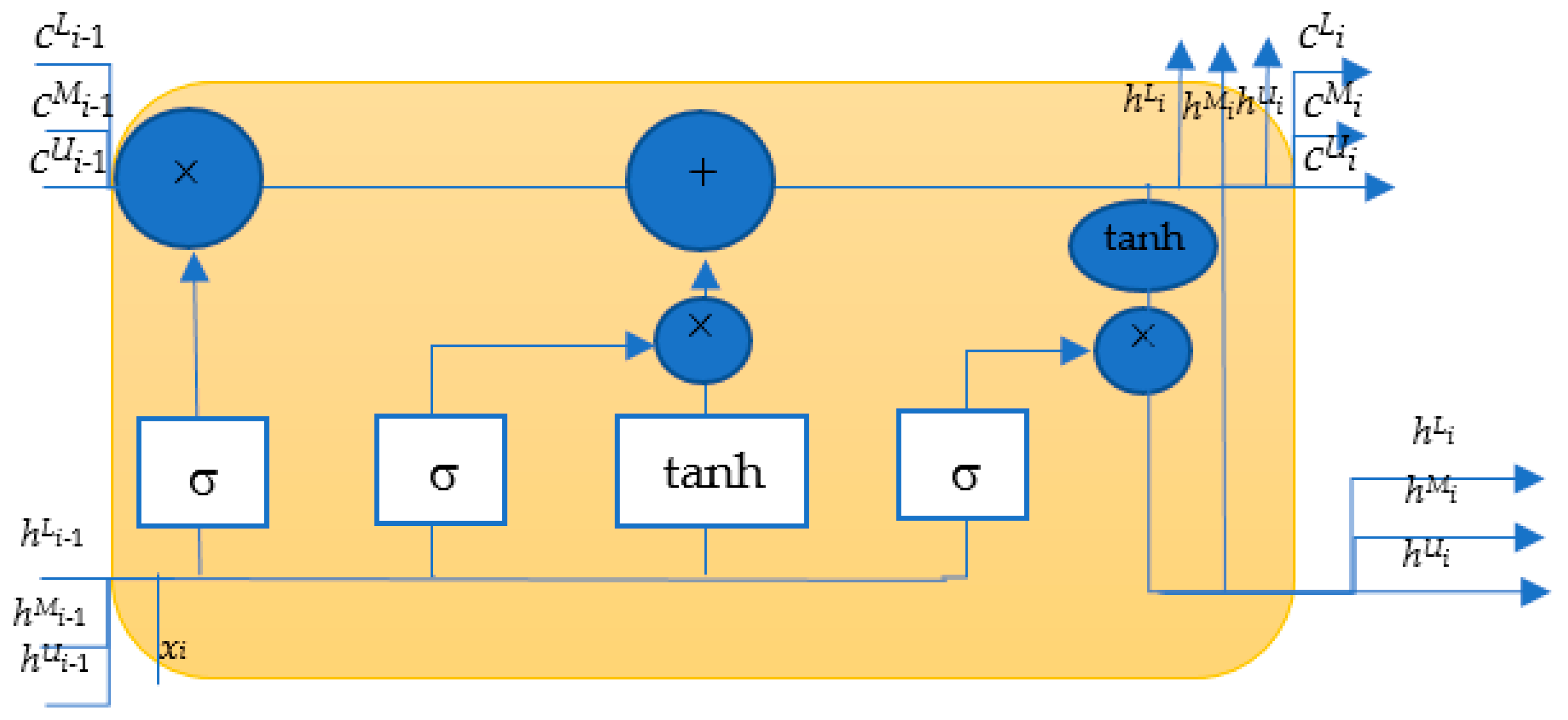To improve the shortcomings of recurrent neural networks, Hochreiter and Schmidhuber [8] proposed the long short-term nemory (LSTM) network in 1997. The long short-term memory model was developed on the basis of recurrent neural networks and is of a cyclical type. LSTM is a neural network architecture that adds the forget gate, input gate, and output gate to the processing unit in the hidden layer, the purpose of which is to read more past information. The model will first determine whether the information is useful, and then decide whether to add or delete the information to increase the ability of the neural network to be reliable over a long period.

Comparing the cyclic neural network and the long short-term memory model, it can be seen that the cyclic neural network will only receive the information calculated in the previous pass, while the long short-term memory model not only receives the information calculated in the last iteration but also all past messages. The long short-term memory model not only retains the advantages of the recurrent neural network but is also able to handle short-term dependencies. Therefore, the LSTM model can solve many tasks that the recurrent neural network could not solve in the past [7]. The development of short-term memory models has thus far provided help in various processing tasks, and they are widely used in various fields such as speech recognition [9,10], handwriting recognition [11], and predictions [12,13,14].

Table 1. Long short-term memory (LSTM) applications from 2015.

Author	Applied Field	Methodology	Compared Methodology
Tian and Pan [15]	Traffic	LSTM	SVR, Random Walker (RW), Fuzzy Neural Network (FNN), and Stacked Autoencoder (SAE)
Liu et al. [16]	Electroencephalography	LSTM	RNN
Janardhanan and Barrett [17]	CPU usage of Google’s data center	LSTM	ARIMA
Siami-Namini et al. [18]	Financial index and economic indexes	LSTM	ARIMA
Phyo et al. [19]	Power load	LSTM	Deep Confidence Network (DBN)
Fan et al. [20]	Production forecasting	Integrates the ARIMA model and the LSTM model.	ARIMA
Shahid et al. [21]	Wind power	GLSTM	LSTM
Zhang et al. [22]	Stock price movement prediction	FA-CNN	LSTM

summarizes the long and short-term memory models used to make predictions in related literature since 2015. Tian and Pan [15] used LSTM to predict the time series of car traffic, and the prediction time interval was divided into four types; the prediction accuracy of the five models was then compared and generalized. The study indicated that the prediction accuracy rate of LSTM was the best. This showed that LSTM has a high predictive ability and high generalization ability and that LSTM is better than RNN. Liu et al. [16] explores the prediction accuracy of LSTM on neonatal brainwave maps with different numbers of neurons. To verify the feasibility of LSTM, the study also compared LSTM with RNN. The results showed that LSTM is better than RNN. Janardhanan and Barrett [17] used LSTM to predict the computer CPU usage of Google’s data center in time series. Based on the results of multiple computers, the mean absolute percentage error (MAPE) value of the LSTM model was 17–23%, and that of the ARIMA model was 37–42%. Siami-Namini et al. [18] adopted LSTM to predict six financial indexes and six economic indexes. In the financial and economic average forecast results, the error rates of LSTM forecasting were 87% and 84% lower than that of ARIMA, respectively. Phyo et al. [19] used LSTM and the Deep Confidence Network (DBN) to predict the power load in Thailand, and the prediction accuracy of the two models was compared. The results showed that LSTM offers better predictive ability. Fan et al. [20] developed an integrated method that combined the ARIMA model with the LSTM model. Shahid et al. [21] developed a novel genetic long short-term memory (GLSTM) method; this method improved wind power predictions from 6% to 30% compared to existing techniques. Zhang et al. [22] developed a convolutional neural network model based on a deep factorization machine and attention mechanism (FA-CNN). The results indicated that FA-CNN obtained better performance than the traditional LSTM.

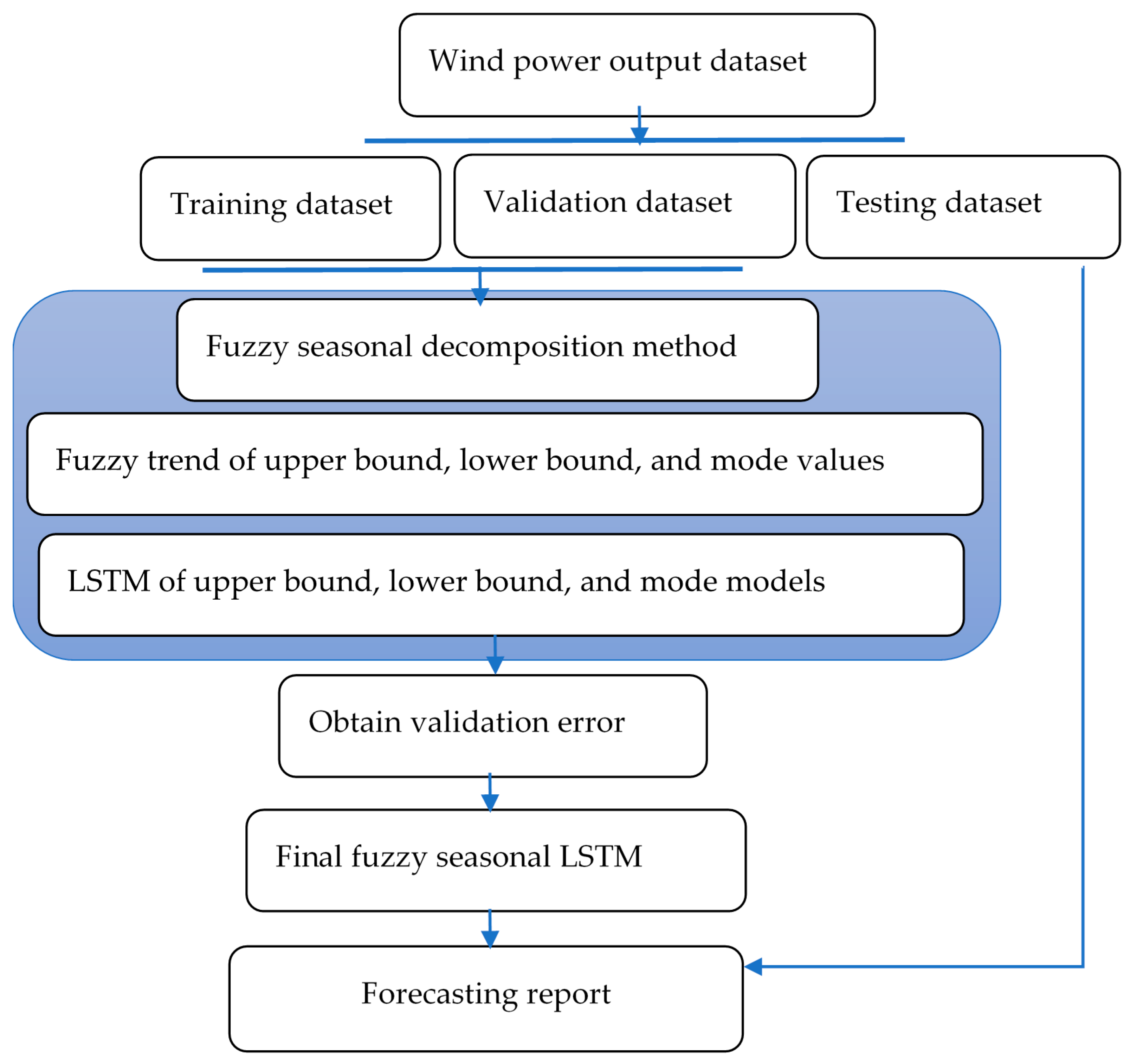
In this study, the prediction model adopts three LSTMs with fuzzy seasonal indexes to approach the fuzzy set’s upper and lower bounds, respectively, as well as mode prediction values. This is a novel prediction model for wind power output forecasting. The rest of this paper is organized as follows. Section 2 introduces the fuzzy seasonal LSTM (FSLSTM) in detail, which include fuzzy seasonal decomposition and fuzzy LSTM technology. Section 3 presents the experimental results of the FSLSTM for wind power output prediction. Finally, we draw conclusions and make suggestions for future research in Section 4.

2. Fuzzy Seasonal LSTM for Wind Power Output

In this study, the wind power output dataset is examined. This dataset is further divided into training, validation, and testing datasets, respectively. Firstly, the fuzzy seasonal index is calculated by seasonal trend decomposition. This method can define the fuzzy seasonal membership function with time series, and then the fuzzy trend dataset can be estimated using the multiplicative model. LSTM is employed to predict the fuzzy trend datasets for the upper bound, lower bound, and mode values. Based on the fuzzy LSTM and fuzzy seasonal index, the final forecasting report can be obtained using the measure index. A flowchart of the fuzzy seasonal LSTM for wind power output is shown in Figure 1.

2.1. Fuzzy Seasonal Decomposition

Chang [21] proposed the fuzzy seasonality index $S_k^{*}$, which is defined as possessing a triangular membership function, from the seasonality index set. Chang [23] determined $S_k^{*}$ as follows:

$$\begin{array}{l}{S}_k^{*}=(s_k^L,s_k^M,s_k^U)=(\min (s_{k+(T-W+1)\times m},s_{k+(T-W+2)\times m},\dots ,s_{k+T\times m}),\\ s_k,\max (s_{k+(T-W+1)\times m},s_{k+(T-W+2)\times m},\dots ,s_{k+T\times m})),k=1,\dots ,m\end{array}$$

(1)

where $s_k^L,s_k^M,s_k^U$ are the W-period lower bound, W-period smoothing-operators (1 ≤ W ≤ T), and W-period upper bound, respectively.

In a time-series problem, reducing seasonality for time series predictions is very important. The fuzzy seasonality index has been shown to effectively obtain good performance in time series predictions. Therefore, this study proposes a novel fuzzy seasonal LSTM that uses the fuzzy seasonality index and a decomposition method to solve the seasonal time series problem. The multiplicative model is employed in the time series problem. Moreover, the IFLR with a spread unrestricted model is combined with symmetrical triangular FNs for forecasting and can obtain an accurately estimated value using Equation (3). Therefore, in the proposed model, a multiplicative model is used to obtain FNs based on a fuzzy seasonality index, as follows:

$$\widetilde{F_{k+(T+v)}^I}=(f_{k+(T+v)}^{LTr}\times s_k^L\times \epsilon ,f_{k+(T+v)}^{MTr}\times s_k^M\times \epsilon ,f_{k+(T+v)}^{UTr}\times s_k^U\times \epsilon )$$

(2)

where $\widetilde{F_{k+(T+v)}}$ represents the fuzzy seasonal LSTM forecast value, $f_{k+(T+v)}^{LTr}$ is the lower-bound estimated value of the trend, $f_{k+(T+v)}^{MTr}$ is the mode estimated value of the trend, $f_{k+(T+v)}^{UTr}$ is the upper-bound estimated value of the trend, and ε is the model noise. The proposed fuzzy seasonal LSTM model can effectively use fuzzy seasonal decomposition to reduce seasonal effects in time series problems.

2.2. Fuzzy Seasonal LSTM Model

In the fuzzy seasonal LSTM model, the fuzzy trend lower bound, upper bound, and mode values must be trained. Therefore, the construction of the fuzzy LSTM method with the input lower bound of {(x_i,$f_i^{LTr}$), i = 1, 2, …, N}, mode {(x_i,$f_i^{MTr}$), i = 1, 2, …, N}, and the upper bound of {(x_i,$f_i^{UTr}$), i = 1, 2, …, N}, respectively, can be represented as follows:

$$f_{LTr}(x_i)=Y_i^L=o_{Li}\otimes \tan h(c_{Li})$$

(3)

$$f_{MTr}(x_i)=Y_i^M=o_{Mi}\otimes \tan h(c_{Mi})$$

(4)

$$f_{UTr}(x_i)=Y_i^U=o_{Ui}\otimes \tan h(c_{Ui})$$

(5)

where the fuzzy long-term state $\tilde{c}$ is (c_Li, c_Mi, c_Ui), and the output gate $\tilde{o}$ (o_Li, o_Mi, o_Ui) can be estimated.

A fully connected fuzzy LSTM unit contains four layers, as with the traditional LSTM, and the fuzzy input vector (x_i) and previous fuzzy short-term memory ($\widetilde{h_i{}_{-1}}$) are imported into these four layers (Figure 2). $\widetilde{g_i}$ is the main layer of the fuzzy LSTM and uses the tanh activation function, and the fuzzy output data are stored in fuzzy long-term memory ${\tilde{c}}_i$. The other three layers use logic activation functions, and their output ranges from 0 to 1. ${\tilde{f}}_i$f_i is the fuzzy forget gate that controls which parts of long-term memory should be deleted. ${\tilde{I}}_i$ is the fuzzy input gate that determines which parts of the fuzzy input should be added. $\widetilde{o_i}$ is the gate that controls which parts of the fuzzy long-term memory should be read and the fuzzy output at this time step, $f_i^{LTr}=h_i^L$, $f_i^{MTr}=h_i^M$, and $f_i^{UTr}=h_i^U$.

The operation can be written as follows:

Fuzzy input gate:

$$\widetilde{I_i}=(\sigma (W_{x_{LI}}^T{x}_{Li}+W_{h_{LI}}^T{h}_L(i-1)+b_{LI}),\sigma (W_{x_{MI}}^T{x}_{Mi}+W_{h_{MI}}^T{h}_M(i-1)+b_{Mi}),\sigma (W_{x_{UI}}^T{x}_{Ui}+W_{hI}^T{h}_U(i-1)+b_{UI}))$$

(6)

Fuzzy forget gate:

$$\widetilde{f_i}=(\sigma (W_{x_{Lf}}^T{x}_{Li}+W_{hf}^T{h}_L(i-1)+b_{Lf}),\sigma (W_{x_{Mf}}^T{x}_{Mi}+W_{h_{Mf}}^T{h}_M(i-1)+b_{Mf}),\sigma (W_{x_{Uf}}^T{x}_{Ui}+W_{h_{Uf}}^T{h}_U(i-1)+b_{Uf}))$$

(7)

Output gate:

$$\widetilde{o_i}=(\sigma (W_{x_{Lo}}^T{x}_{Li}+W_{ho}^T{h}_L(i-1)+b_{Lo}),\sigma (W_{x_{Mo}}^T{x}_{Mi}+W_{h_{Mo}}^T{h}_M(i-1)+b_{Mo}),\sigma (W_{x_{Uo}}^T{x}_{Ui}+W_{h_{Uo}}^T{h}_U(i-1)+b_{Uo}))$$

(8)

Neuron input and cell input:

$$\widetilde{g_i}=(\sigma (W_{x_{Lg}}^T{x}_{Li}+W_{hg}^T{h}_L(i-1)+b_{Lg}),\sigma (W_{x_{Mg}}^T{x}_{Mi}+W_{h_{Mg}}^T{h}_M(i-1)+b_{Mg}),\sigma (W_{x_{Ug}}^T{x}_{Ui}+W_{h_{Ug}}^T{h}_U(i-1)+b_{Ug}))$$

(9)

where $\widetilde{W_{xI}=(}{W}_{x_{LI}}^T,W_{x_{MI}}^T,W_{x_{UI}}^T)$, $\widetilde{W_{xf}=(}{W}_{x_{Lf}}^T,W_{x_{Mf}}^T,W_{x_{Uf}}^T)$, $\widetilde{W_{xo}=(}{W}_{x_{Lo}}^T,W_{x_{Mo}}^T,W_{x_{Uo}}^T)$, and $\widetilde{W_{xg}=(}{W}_{x_{Lg}}^T,W_{x_{Mg}}^T,W_{x_g}^T)$ are the fuzzy weight matrices of each of the four layers used for their connections with the fuzzy input vector, and the fuzzy weight matrices are connected to the fuzzy short-term state $\widetilde{h_i{}_{-1}}$.$b_i,b_f,b_o,b_g$ $\widetilde{b_I=(}{b}_{LI},b_{MI},b_{UI})$, $\widetilde{b_f=(}{b}_{Lf},b_{Mf},b_{Uf})$, $\widetilde{b_o=(}{b}_{Lo},b_{Mo},b_{Uo})$ and $\widetilde{b_g=(}{b}_{Lg},b_{Mg},b_{Ug})$ are the deviation terms of each of the four layers, tanh is the hyperbolic tangent function (e^(x) − e^(−x))/(e^(x) + e^(−x)), and σ is the sigmoid function 1/(1 + e^(−x)).

Finally, the long-term and short-term states are calculated as follows:

Fuzzy long-term state:

$$\widetilde{c_i}=\widetilde{f_i}\times \widetilde{c_{i-1}}+\widetilde{I_i}\times \widetilde{g_i}$$

(10)

Fuzzy short-term state:

$$\widetilde{Y_i}=\widetilde{h_i}=\widetilde{o_i}\times \tanh (\widetilde{c_i})$$

(11)

Moreover, this FSLSTM adopts the adaptive moment estimation (Adam) optimization algorithm from Kingma and Ba [24], which employs stochastic optimization, to search for the proper parameters of the FSLSTM. The Adam optimization algorithm was demonstrated empirically to show that convergence meets the expectations of the theoretical analysis. The proposed FSLSTM can achieve robust performance based on the Adam optimization algorithm. The maximum epochs, initial parameters learning rate, gradient threshold, learn rate drop period, and learn rate drop factor of FSLSTM are 250, 0.005, 1, 125, and 0.2, respectively.

3. A Wind Power Output Example and Empirical Results

Energy conservation and decreasing carbon are very important management issues for the global power industry. To demonstrate its concern regarding the global warming issue and to comply with the government’s Sustainable Energy Guidelines, the Taiwanese government is actively promoting the use of clean energy. The Taipower company has built 17 wind energy power stations in Taiwan that record monthly data on the total power output. All experimental data can be download from the National Development Council in Taiwan (https://data.gov.tw (accessed on 21 July 2020)). In this study, we selected three wind energy power stations: the Shimen, Taichung, and Mailiao wind power plants. Figure 3 and

Table 2. The actual power output of the three wind power stations (units: kilowatt-hours).

Date	Shimen	Taichung	Mailiao
2017/01	463,283	696,640	16,804,318
2017/02	407,258	630,978	14,938,148
2017/03	419,363	440,900	10,740,085
2017/04	336,234	220,980	6,313,574
2017/05	350,142	166,390	3,919,309
2017/06	195,069	124,600	4,899,275
2017/07	172,429	78,330	2,342,427
2017/08	349,341	92,620	2,677,669
2017/09	330,570	109,600	2,426,662
2017/10	1,239,911	599,700	13,307,824
2017/11	741,605	516,784	14,782,631
2017/12	987,529	688,270	12,469,649
2018/01	699,627	578,820	14,875,834
2018/02	573,615	527,320	12,316,626
2018/03	428,185	339,634	8,437,488
2018/04	267,650	169,866	4,483,353
2018/05	260,618	127,692	3150,546
2018/06	268,476	217,353	6,132,870
2018/07	461,025	113,979	2,889,834
2018/08	197,814	81,125	3,290,543
2018/09	391,113	289,650	8,800,633
2018/10	631,983	627,877	14,854,486
2018/11	498,720	381,956	9,282,346
2018/12	791,605	722,624	18,553,027
2019/01	737,047	719,896	18,322,239
2019/02	520,684	408,360	9,729,809
2019/03	651,798	328,996	7,658,895
2019/04	388,595	207,114	5,157,800
2019/05	386,277	199,886	4,300,127
2019/06	159,193	109,585	2,964,455
2019/07	211,329	149,040	3,339,550
2019/08	339,098	178,123	5,414,371
2019/09	589,619	418,682	9,185,376
2019/10	491,982	541,496	11,115,453
2019/11	845,222	659,646	15,558,639
2019/12	664,395	340,702	14,464,274
2020/01	482,289	421,826	12,276,955
2020/02	398,281	396,284	9,756,250
2020/03	345,802	328,177	8,338,542
2020/04	531,022	347,579	6,938,541
2020/05	192,987	81,714	2,937,135
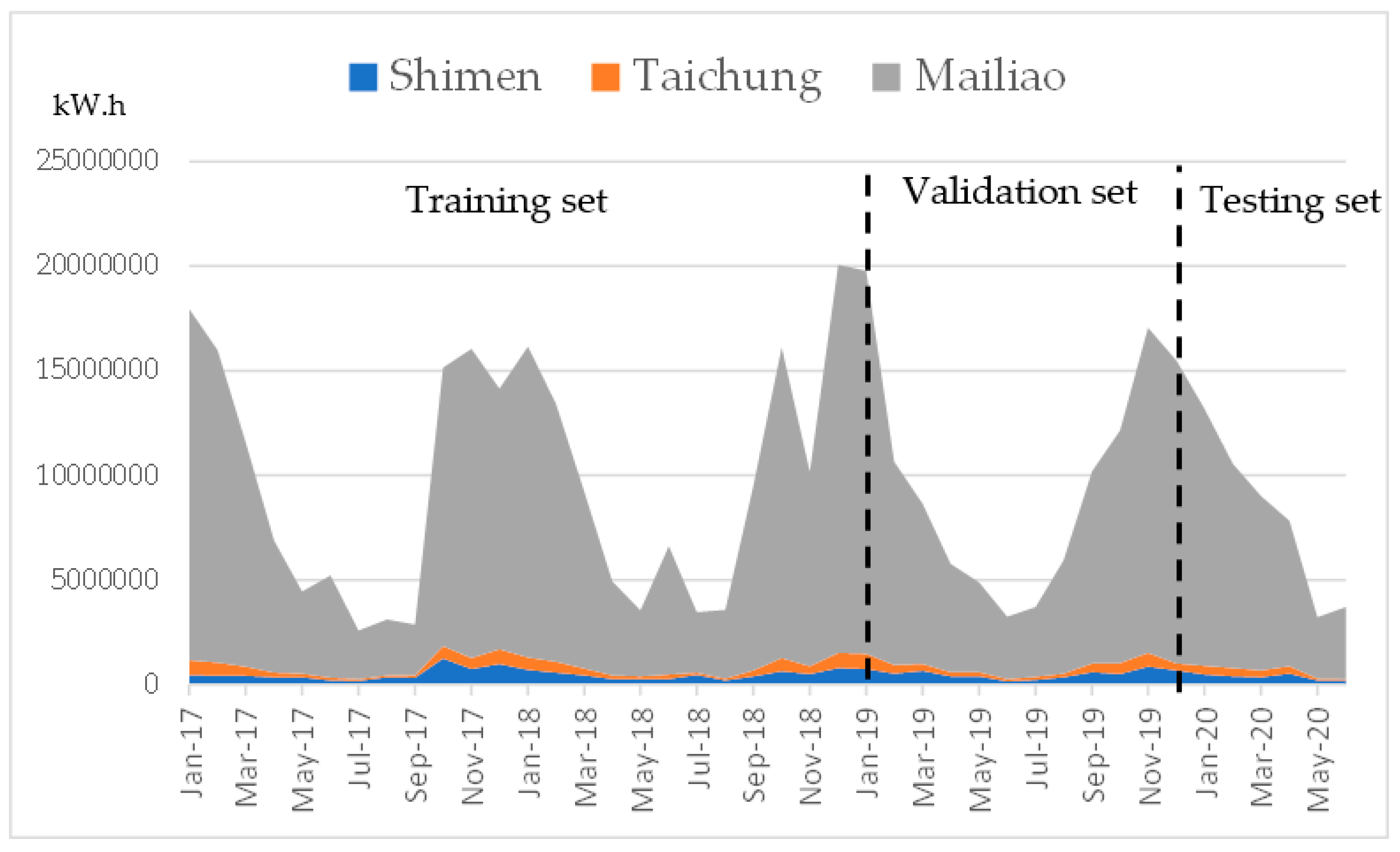
2020/06	195,061	63,884	3,445,273

depict the monthly generated output power (units: kilowatt-hours) from these wind power stations during the period from January 2017 to June 2020 (the total number is 42). In this study, the monthly data were divided into three sets: firstly, a training set was employed to determine the optimum forecasting model during the period from January 2017 to December 2018 (the number of samples in the training set was 24); secondly, a validation set was employed to prevent the overfitting of the different models during the period from January 2019 to December 2019 (the number of samples in the validation set was 24); finally, a testing set was employed to investigate the performance of the different models during the period from January 2020 to June 2020 (the number of samples in the testing set was 24). The percentages of training, validation, and testing sets were 57%, 29%, and 14%, respectively.

Figure 3 clearly indicates that the measured time series feature seasonal data and three types of cycles for the different wind power plants. The Mailiao wind power plant can generate greater power because the Mailiao wind power plant features the largest number of wind-driven generators in Taiwan. Moreover, a larger power output can be obtained during winter in Taiwan as a result of the northeast monsoon.

Table 3. The fuzzy seasonality index of the three wind power stations.

Fuzzy Seasonality Index	Shimen			Taichung			Mailiao
	${\mathit{s}}_{\mathit{k}}^{\mathit{L}}$	${\mathit{s}}_{\mathit{k}}^{\mathit{M}}$	${\mathit{s}}_{\mathit{k}}^{\mathit{U}}$	${\mathit{s}}_{\mathit{k}}^{\mathit{L}}$	${\mathit{s}}_{\mathit{k}}^{\mathit{M}}$	${\mathit{s}}_{\mathit{k}}^{\mathit{U}}$	${\mathit{s}}_{\mathit{k}}^{\mathit{L}}$	${\mathit{s}}_{\mathit{k}}^{\mathit{M}}$	${\mathit{s}}_{\mathit{k}}^{\mathit{U}}$
k = 1	0.6785	1.4709	1.4709	0.5272	1.9039	1.9039	0.5243	1.8802	1.8802
k = 2	0.6785	1.1148	1.1148	0.4536	1.3659	1.3659	0.4055	1.2493	1.2493
k = 3	0.4611	1.1029	1.1029	0.4536	0.9512	0.9512	0.4055	0.8875	0.8875
k = 4	0.4464	0.6785	0.6810	0.2734	0.5272	0.5272	0.3072	0.5243	0.5243
k = 5	0.4464	0.6810	0.6848	0.2497	0.4536	0.4667	0.3072	0.4055	0.4979
k = 6	0.4464	0.4611	0.8694	0.2497	0.4667	0.5819	0.3072	0.4979	0.9466
k = 7	0.4464	0.4464	1.3626	0.2497	0.2734	1.8128	0.3072	0.3072	1.5730
k = 8	0.6848	0.6848	1.4587	0.2497	0.2497	1.8128	0.3484	0.3484	1.7477
k = 9	0.8694	0.8694	1.6686	0.5819	0.5819	2.0790	0.9466	0.9466	1.7477
k = 10	1.3626	1.3626	1.6686	1.3342	1.8128	2.0790	1.5730	1.5730	1.8802
k = 11	1.1148	1.4587	1.6686	1.3342	1.3342	2.0790	1.2493	1.7477	1.8802
k = 12	1.1029	1.6686	1.6686	0.9512	2.0790	2.0790	0.8875	1.6318	1.8802

depict the fuzzy seasonality index with k ranging from 1 to 12 from the selected wind power stations. In addition, the mean absolute percentage error MAPE(%) was used to measure the forecasting accuracy. Equation (12) illustrates the expression of MAPE(%):

$$MAPE(\%)=\frac{100}{M}{\displaystyle \sum _{i=1}^M\left|\frac{A_i-P_i}{A_i}\right|}$$

(12)

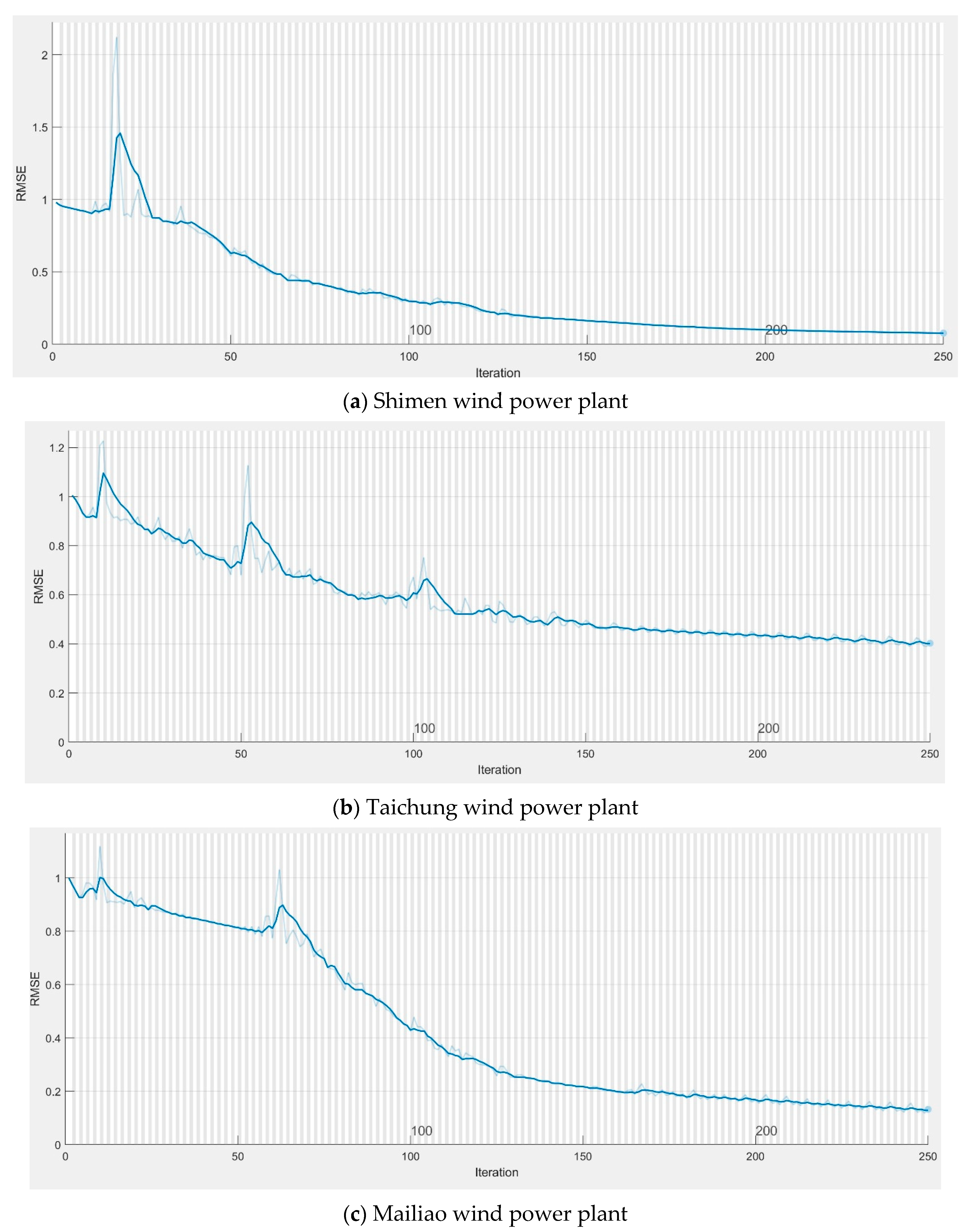
where M is the number of forecasting periods, A_i is the actual production value at period i, and P_i is the forecasting production value at period i. Moreover, the RMSE is employed to evaluate the training error of FSLSTM, which can be expressed as follows:

$$\mathrm{RMSE}=\sqrt{\frac{1}{M}{\displaystyle \sum _{i=1}^M{\left(A_i-P_i\right)}^2}}$$

(13)

Figure 4 shows the training error of the FSLSTM in three wind power stations, adopting the Adam algorithm. We can observe that the FSLSTM can obtain a lower RMSE training error (smaller than 0.2) in three wind power stations.

In this study, the FSLSTM, LSTM [8], ARIMA(1, 0, 0) [25], generalized regression neural network (GRNN) [26], back propagation neural network (BPNN) [27], least square support vector regression (LSSVR) [28], and seasonal autoregressive integrated moving average (SARIMA (1, 0, 0) (1, 0, 0)₁₂) [25] models were used to forecast the monthly wind power output datasets in selected stations in Taiwan. The construction of LSTM is similar to that of the FSLSTM (see Section 2.1). The LSTM network also adopted the Adam optimization algorithm to search for optimal parameters. The ARIMA is similar to SARIMA (see Appendix A), with a difference in seasonal parameters. The construction and parameter (σ) of the GRNN is shown in Appendix B. The parameter (σ) of the GRNN was set to 1. In this study, a well-known intelligent computing machine, BPNN, is also adopted to compare prediction models. In the BPNN, the input layer has one input neuron to catch the input patterns, the hidden layer has ten neurons to propagate the intermediate signals, and the output layer has one neuron. For more training assignments in the BPNN, the hyperbolic tangent sigmoid function is employed as the activation function in the hidden layer, the pure-line transfer function is employed in the output layer as the activation function, and the gradient training is adopted as the learning algorithm for the BPNN. The LSSVR is a popular prediction model in time series problems. For the main constructs of the LSSVR, readers can be refer to [28], and the regularization parameter in the experiment was set to 1. The Radial Basis Function (RBF) Kernel Trick was employed in the LSSVR, and the parameter (σ) of the RBF was set to 0.01.

Table 4. Comparison of the training error (RMSE) with various prediction models for different wind power plants.

	FSLTM	LSTM	BPNN	GRNN	LSSVR	ARIMA	SARIMA
Shimen	0.0770	0.1689	508,0396	0	121,188	1,307,183	866,451
Mailiao	0.1324	0.0592	498,9503	0	2,065,173	22,174,287	15,002,000
Taichung	0.4032	0.0129	208,901	0	90,886	980,862	591,422

depicts the training error with various prediction models. The proposed FSLSTM, LSTM, and GRNN approaches could obtain lower training errors, which means that the training models of the three approach achieved better performance.

Table 5. Comparison of the forecasting results for the Shimen wind power plant.

Date	Actual Value	ARIMA	SARIMA	GRNN	BPNN	LSSVR	LSTM	FSLSTM
								M	U	L
2020/01	482,289	265,130	807,339	463,283	484,678	538,345	663,547	644,173	506,533	458,776
2020/02	398,281	264,905	536,142	407,258	484,678	495,248	545,863	488,201	599,497	564,286
2020/03	345,802	264,996	447,263	419,363	484,678	486,974	390,044	482,980	472,889	345,594
2020/04	531,022	264,959	267,414	336,234	484,678	486,252	274,106	297,131	430,324	426,518
2020/05	192,987	264,974	265,935	350,142	484,678	486,224	291,349	298,220	438,839	297,130
2020/06	195,061	264,968	264,577	195,069	484,678	486,223	263,500	201,939	270,340	343,187
MAPE (%)		37.51	42.41	24.26	61.78	64.40	36.97	32.98	46.20	32.69
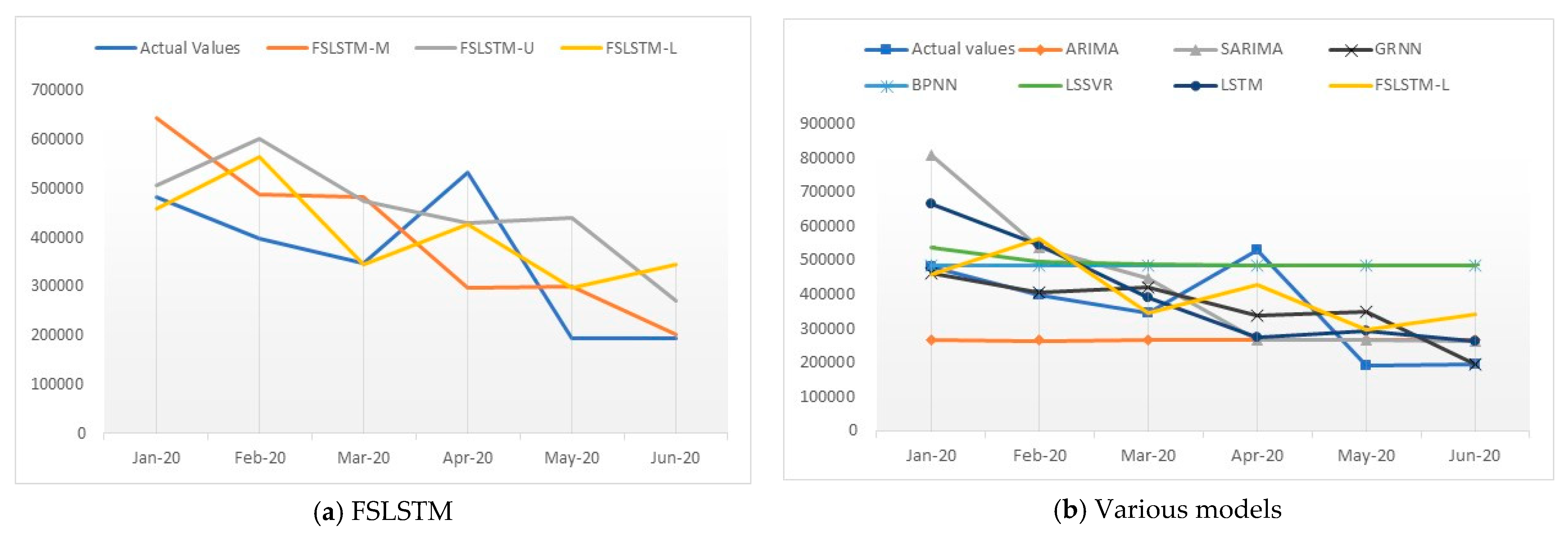
Ranking		(5)	(6)	(1)	(8)	(9)	(4)	(3)	(7)	(2)

illustrates the actual values and experimental results of the FSLSTM model with the mode (M) and upper (U) and lower (L) bounds from January 2020 to June 2020 for the Shimen wind power plant. Figure 5a makes a point-to-point comparison of the actual values and predicted values of FSLSTM. As shown in Figure 4, the peak power output was in April 2020, which was not easily observed in the training dataset. Figure 5b shows a comparison of the actual values and predicted values of ARIMA, SARIMA, GRNN, BPNN, LSTM, and FSLSTM-L for the Shimen wind power plant.

Table 5 shows the experimental results and MAPE(%) obtained by various models. The ranking of MAPE(%) is as follows: GRNN < FSLSTM-L < FSLSTM-M < LSTM < ARIMA < SARIMA < FSLSTM-U < BPNN < LSSVR. Table 4 indicates that the GRNN obtained the smallest MAPE(%), showing the best performance. However, Figure 5 shows that the predicted value of the GRNN could not capture the trend of power output at the Shimen wind power plant. The FSLSTM-L model was able to efficiently capture the trends of the data by using the fuzzy seasonal index, although the MAPE(%) of the FSLSTM-L was higher than that of the GRNN in the example. Thus, the proposed FSLSTM model is suggested to serve as a prediction model for power output for the Shimen wind power plant.

Table 6. Comparison of the forecasting results for the Taichung wind power plant.

Date	Actual Value	ARIMA	SARIMA	GRNN	BPNN	LSSVR	LSTM	FSLSTM
								M	U	L
2020/01	421,826	325,087	901,020	696,640	355,700	355,520	366,148	294,629	678,346	209,460
2020/02	396,284	310,188	319,967	630,978	355,700	355,510	698,414	297,072	479,634	340,958
2020/03	328,177	295,972	370,365	440,900	355,700	355,500	466,354	247,767	297,040	799,896
2020/04	347,579	282,408	186,543	220,980	355,700	355,491	615,672	149,127	170,964	942,933
2020/05	81,714	269,465	209,163	166,390	355,700	355,481	462,467	133,024	502,598	327,882
2020/06	63,884	257,115	104,727	124,600	355,700	355,471	411,278	141,578	161,424	268,070
MAPE(%)		100.9099	68.6577	65.6349	138.1218	151.4939	203.0705	53.5326	134.9830	166.70
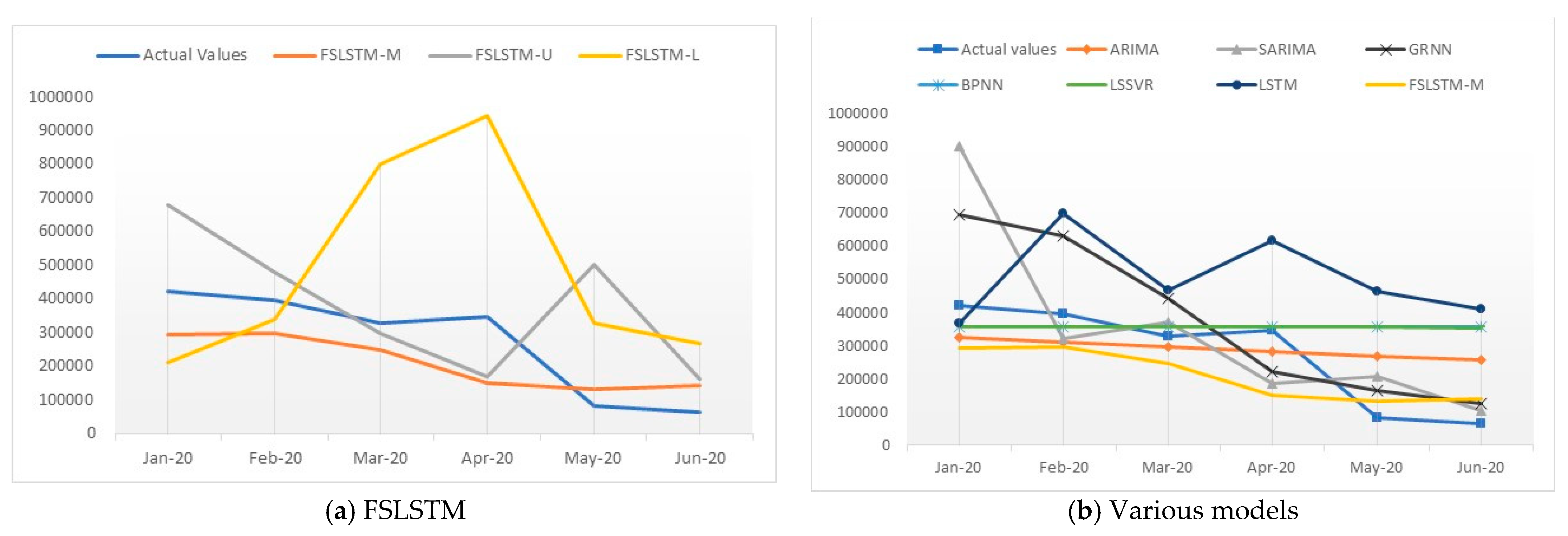
Ranking		(9)	(2)	(4)	(8)	(6)	(5)	(1)	(3)	(7)

illustrates the actual values and experimental results of the proposed model for the Taichung wind power plant. Figure 6a makes a point-to-point comparison between the actual values and predicted values of the FSLSTM at the Taichung wind power plant. Downward trends of power output can be observed in Figure 5. Figure 6b illustrates a comparison between the actual values and predicted values of the ARIMA, SARIMA, GRNN, BPNN, LSTM, and FSLSTM-M models for the Taichung wind power plant.

Table 6 shows the experimental results and MAPE(%) obtained by various models for the Taichung wind power plant. The ranking of MAPE(%) is FSLSTM-M < SARIMA < FSLSTM-U < GRNN < LSTM < LSSVR < FSLSTM-L < BPNN < ARIMA. Table 5 indicates that the FSLSTM-M obtained the smallest MAPE(%), which means that FSLSTM-M achieved the best performance in this example. Moreover, Figure 6 shows that the predicted value of the FSLSTM-M was able to capture the trend of power output at the Taichung wind power plant. Moreover, the two seasonal models, FSLSTM-M and SARIMA, obtained better performance than the other models, possibly because the power output at the Taichung wind power plant has a seasonal influence. Thus, the proposed FSLSTM model is also suggested to serve as a prediction model for power output at the Taichung wind power plant.

Table 7. Comparison of the forecasting results for the Mailiao wind power plant.

Date	Actual Value	ARIMA	SARIMA	GRNN	BPNN	LSSVR	LSTM	FSLSTM
								M	U	L
2020/01	12,276,955	14,382,852	19,238,928	16,804,318	8,886,115	10,655,725	11,490,891	15,802,902	17,649,361	2,738,426
2020/02	9,756,250	14,301,888	9,495,570	14,938,148	8,886,115	9,381,110	9,797,061	8,654,354	11,218,379	7,435,086
2020/03	8,338,542	14,221,379	7,698,419	10,740,085	8,886,115	9,060,788	3,481,336	8,168,194	6,652,353	21,668,492
2020/04	6,938,541	14,141,324	5,138,157	6,313,574	8,886,115	9,027,759	1,163,317	5,596,075	3,765,754	16,162,712
2020/05	2,937,135	14,061,720	4,296,410	3,919,309	8,886,115	9,026,361	5,262,665	3,750,842	2,366,479	2,354,684
2020/06	3,445,273	13,982,563	2,959,347	4,899,275	8,886,115	9,026,337	3,460,068	3,445,273	3,011,638	2,864,925
MAPE(%)		153.7846	25.5645	33.9068	71.9399	70.8555	37.9852	14.8515	26.1184	71.8270
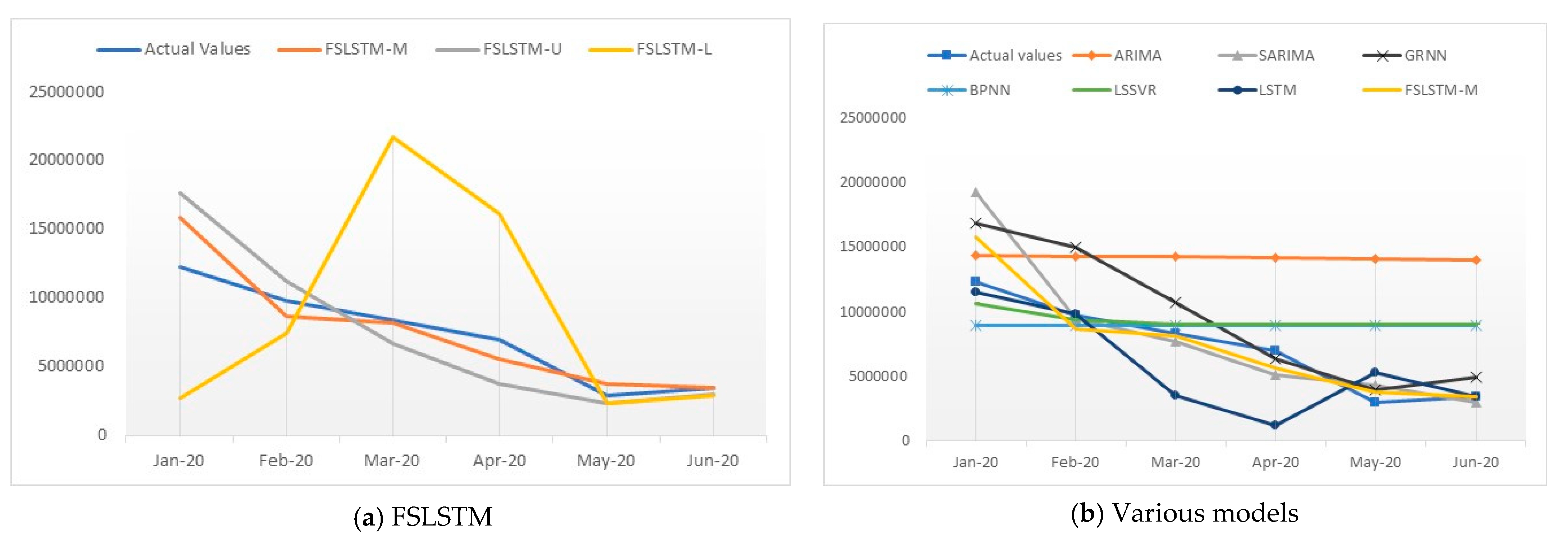
Ranking		(9)	(2)	(4)	(8)	(6)	(5)	(1)	(3)	(7)

illustrates the actual values and experimental results of the proposed model for the Mailiao wind power plant. Figure 7a also makes a point-to-point comparison of the actual values and predicted values of FSLSTM at the Mailiao wind power plant. As with the Taichung wind power plant, downward trends of power output can be observed in Figure 7 for the Mailiao wind power plant. Because the Mailiao wind power plant provides a larger quantity of wind power generation than the other power plants, Mailiao outputs more power in KWh. Figure 7b shows a comparison between the actual values and predicted values of ARIMA, SARIMA, GRNN, BPNN, LSTM, and FSLSTM-M models at the Mailiao wind power plant.

Table 7 shows the experimental results and MAPE(%) obtained using various models for the Mailiao wind power plant. The ranking of MAPE(%) is FSLSTM-M < SARIMA < FSLSTM-U < GRNN < LSTM < LSSVR < FSLSTM-L < BPNN < ARIMA. Table 6 indicates that the FSLSTM-M obtained the smallest MAPE(%), which means that the FSLSTM-M achieved the best performance in this example. Both seasonal models, FSLSTM-M and SARIMA, obtained better performance than the other models and were able to capture the trend of power output for the Mailiao wind power plant, possibly for the same reasons as those of the Taichung wind power plant. Moreover, the Mailiao region is very close to the Taichung region in Taiwan. Thus, the ranking of MAPE(%) in the Mailiao region is the same as that of the Taichung region. Again, the proposed FSLSTM model is suggested to serve as a prediction model for wind power output at the Mailiao wind power plant.

By reviewing the three forecasting examples using the FSLSTM model, some findings can be concluded, as follows: (1) the FSLSTM model can efficiently handle seasonal influence. In the Taichung and Mailiao regions, the seasonal influence of wind power output can be observed. (2) In all examples, the FSLSTM model could obtain better performance and more accurately capture the trends of wind power output. This performance was not observed for the traditional LSTM in the three examples. (3) For the three different types of wind power output, the FSLSTM-M model obtained better performance than almost all other models. The FSLSTM-M model is thus recommended as a prediction model for wind power output.

4. Managerial Implications

A wind power forecasting system is implemented for the government in this study. The government can use the forecasting results of monthly wind power output to reduce the risk of insufficient power supply. The wind power forecasting system can provide an early warning of insufficient power supply to decision-makers in the government to reduce the risk of an insufficient power supply. The government has developed an offshore wind power facility, the main goal of which is to generate enough electricity so that renewable energy can replace nuclear power generation. The mechanism of early warning by the proposed wind power forecasting system can accurately predict the wind power output. The decision-makers in the government can therefore conduct proper planning to avoid the risk of an insufficient power supply.

5. Conclusions

Due to the Sustainable Development Goals, wind power prediction has become increasingly crucial in Taiwan. Moreover, LSTM models have been successfully used in time series forecasting problems. However, they have not been widely explored in seasonal time series prediction. This study developed a novel FSLSTM model to exploit the unique strength of the fuzzy seasonal index and the LSTM technique in order to predict wind power output in Taiwan. In all examples, the FSLSTM model could obtain better performance and more accurately capture the trends of wind power output. This performance was not observed for the traditional LSTM in the three examples. The simultaneous results indicate that the FSLSTM model represents a promising alternative for analyzing wind power output in Taiwan. The superior performance of the FSLSTM model can be ascribed to two causes: first, the FSLSTM benefits from the advantages of LSTM and can effectively capture the time series dataset by the mechanism of a recurrent neural network; second, the fuzzy decomposition method enhances the ability of the FSLSTM models to capture seasonal nonlinear data patterns under an uncertain environment. The limitation of the FSLSTM model is that it is only suitable for strong monthly seasonal patterns. Forecasting other types of time series data using an LSTM-related model would be a challenging issue for future studies. Future research directions could consider using data preprocessing techniques to achieve improvements in the forecasting accuracy of the FSLSTM model for seasonal time series data. The parameters of FSLSTM also could be searched by a heuristic algorithm to improve the performance.

References

1. Liu, F.; Li, R.; Dreglea, A. Wind speed and power ultra short-term robust forecasting based on Takagi–Sugeno fuzzy model. Energies 2019, 12, 3551. [Google Scholar] [CrossRef] [Green Version]
2. Liu, F.; Li, R.; Li, Y.; Cao, Y.; Panasetsky, D.; Sidorov, D. Short-term wind power forecasting based on TS fuzzy model. In Proceedings of the 2016 IEEE PES Asia-Pacific Power and Energy Engineering Conference (APPEEC), Xi’an, China, 25–28 October 2016; pp. 414–418. [Google Scholar]
3. Yu, C.; Li, Y.; Bao, Y.; Tang, H.; Zhai, G. A novel framework for wind speed prediction based on recurrent neural networks and support vector machine. Energy Convers. Manag. 2018, 178, 137–145. [Google Scholar] [CrossRef]
4. Zjavka, L.; Mišák, S. Direct wind power forecasting using a polynomial decomposition of the general differential equation. IEEE Trans. Sustain. Energy 2018, 9, 1529–1539. [Google Scholar] [CrossRef]
5. Liu, H.; Mi, X.; Li, Y. Smart deep learning based wind speed prediction model using wavelet packet decomposition, convolutional neural network and convolutional long short term memory network. Energy Convers. Manag. 2018, 166, 120–131. [Google Scholar] [CrossRef]
6. Toubeau, J.-F.; Dapoz, P.-D.; Bottieau, J.; Wautier, A.; De Grève, Z.; Vallée, F. Recalibration of recurrent neural networks for short-term wind power forecasting. Electr. Power Syst. Res. 2021, 190, 106639. [Google Scholar] [CrossRef]
7. Gers, F.A.; Schmidhuber, J.; Cummins, F. Learning to forget: Continual prediction with LSTM. In Proceedings of the Ninth International Conference on Artificial Neural Networks, Edinburgh, UK, 7–10 September 1999; pp. 850–855. [Google Scholar]
8. Hochreiter, S.; Schmidhuber, J. Long short-term memory. Neural Comput. 1997, 9, 1735–1780. [Google Scholar] [CrossRef] [PubMed]
9. Graves, A.; Mohamed, A.; Hinton, G. Speech recognition with deep recurrent neural networks. In Proceedings of the 2013 IEEE International Conference on Acoustics, Speech and Signal Processing, Vancouver, BC, Canada, 26–31 May 2013; pp. 6645–6649. [Google Scholar]
10. Sak, H.; Senior, A.; Beaufays, F. Long short-term memory based recurrent neural network architectures for large vocabulary speech recognition. arXiv 2014, arXiv:1402.1128. [Google Scholar]
11. Graves, A.; Schmidhuber, J. Offline Arabic Handwriting Recognition with Multidimensional Recurrent Neural Networks. In Proceedings of the Twenty-Second Annual Conference on Neural Information Processing Systems, Vancouver, BC, Canada, 8–11 December 2008; pp. 1–8. [Google Scholar]
12. Duan, Y.; Lv, Y.; Wang, F. Travel time prediction with LSTM neural network. In Proceedings of the 2016 IEEE 19th International Conference on Intelligent Transportation Systems (ITSC), Rio de Janeiro, Brazil, 1–4 November 2016; pp. 1053–1058. [Google Scholar]
13. Nelson, D.M.Q.; Pereira, A.C.M.; de Oliveira, R.A. Stock market’s price movement prediction with LSTM neural networks. In Proceedings of the 2017 International Joint Conference on Neural Networks (IJCNN), Anchorage, AK, USA, 14–19 May 2017; pp. 1419–1426. [Google Scholar]
14. Abdel-Nasser, M.; Mahmoud, K. Accurate photovoltaic power forecasting models using deep LSTM-RNN. Neural Comput. Appl. 2019, 31, 2727–2740. [Google Scholar] [CrossRef]
15. Tian, Y.; Pan, L. Predicting short-term traffic flow by long short-term memory recurrent neural network. In Proceedings of the 2015 IEEE International Conference on Smart City/SocialCom/SustainCom (SmartCity), Chengdu, China, 19–21 December 2015; pp. 153–158. [Google Scholar]
16. Liu, L.; Chen, W.; Cao, G. Prediction of neonatal amplitude-integrated EEG based on LSTM method. In Proceedings of the 2016 IEEE International Conference on Bioinformatics and Biomedicine (BIBM), Shenzhen, China, 15–18 December 2016; pp. 497–500. [Google Scholar]
17. Janardhanan, D.; Barrett, E. CPU workload forecasting of machines in data centers using LSTM recurrent neural networks and ARIMA models. In Proceedings of the 12th International Conference for Internet Technology and Secured Transactions (ICITST), Cambridge, UK, 11–14 December 2017; pp. 55–60. [Google Scholar]
18. Siami-Namini, S.; Tavakoli, N.; Namin, A.S. A comparison of ARIMA and LSTM in forecasting time series. In Proceedings of the 17th IEEE International Conference on Machine Learning and Applications (ICMLA), Orlando, FL, USA, 17–20 December 2018; pp. 1394–1401. [Google Scholar]
19. Phyo, P.P.; Jeenanunta, C.; Hashimoto, K. Electricity Load Forecasting in Thailand Using Deep Learning Models. Int. J. Electr. Electron. Eng. Telecommun. 2019, 8, 221–225. [Google Scholar] [CrossRef]
20. Fan, D.; Sun, H.; Yao, J.; Zhang, K.; Yan, X.; Sun, Z. Well production forecasting based on ARIMA-LSTM model considering manual operations. Energy 2021, 220, 119708. [Google Scholar] [CrossRef]
21. Shahid, F.; Zameer, A.; Muneeb, M. A novel genetic LSTM model for wind power forecast. Energy 2021, 223, 120069. [Google Scholar] [CrossRef]
22. Zhang, X.; Liu, S.; Zheng, X. Stock Price Movement Prediction Based on a Deep Factorization Machine and the Attention Mechanism. Mathematics 2021, 9, 800. [Google Scholar] [CrossRef]
23. Chang, P.-T. Fuzzy seasonality forecasting. Fuzzy Sets Syst. 1997, 90, 1–10. [Google Scholar] [CrossRef]
24. Kingma, D.P.; Ba, L.J. Adam: A Method for Stochastic Optimization. In Proceedings of the International Conference on Learning Representations (ICLR), San Diego, CA, USA, 7–9 May 2015; pp. 1–13. [Google Scholar]
25. Box, G.; Jenkins, G. Time Series Analysis: Forecasting and Control; Holden-Day: San Francisco, CA, USA, 1976. [Google Scholar]
26. Specht, D.F. A general regression neural network. IEEE Trans. Neural Netw. 1991, 2, 568–576. [Google Scholar] [CrossRef] [PubMed] [Green Version]
27. Pai, P.-F.; Lin, K.-P. Application of neural fuzzy systems in reliability prediction. Qual. Reliab. Eng. Int. 2006, 22, 199–211. [Google Scholar] [CrossRef]
28. Van Gestel, T.; Suykens, J.A.K.; Baestaens, D.-E.; Lambrechts, A.; Lanckriet, G.; Vandaele, B.; De Moor, B.; Vandewalle, J. Financial time series prediction using least squares support vector machines within the evidence framework. IEEE Trans. Neural Netw. 2001, 12, 809–821. [Google Scholar] [CrossRef] [PubMed] [Green Version]
Figure 1. A flowchart of the fuzzy seasonal LSTM prediction model.
Mathematics 09 01178 g001
Figure 2. A construction diagram of the fuzzy LSTM prediction model.
Mathematics 09 01178 g002
Figure 3. Illustration of the actual power output of the three wind power stations.
Mathematics 09 01178 g003
Figure 4. Illustration of the training error of the FSLSTM for the three wind power stations.
Mathematics 09 01178 g004
Figure 5. Illustration of the actual and forecasted power outputs of various models for the Shimen wind power plant.
Mathematics 09 01178 g005
Figure 6. Illustration of the actual and forecasting power outputs of various models for the Taichung wind power plant.
Mathematics 09 01178 g006
Figure 7. Illustration of the actual and forecasting power output of various models for the Mailiao wind power plant.
Mathematics 09 01178 g007