Article

Integrated Structure-Control Design of a Bipedal Robot Based on Passive Dynamic Walking

by
Josué Nathán Martínez-Castelán
and
Miguel Gabriel Villarreal-Cervantes
*,†
Mecatronic Section, Postgraduate Department, Instituto Politécnico Nacional, CIDETEC, Mexico City 07700, Mexico
*
Author to whom correspondence should be addressed.
These authors contributed equally to this work.
Mathematics 2021, 9(13), 1482; https://doi.org/10.3390/math9131482
Submission received: 26 May 2021 / Revised: 18 June 2021 / Accepted: 19 June 2021 / Published: 24 June 2021
(This article belongs to the Special Issue Numerical Analysis and Scientific Computing)

Abstract

:
The design of bipedal robots is generally fulfilled through considering a sequential design approach, where a synergistic relationship between its structure and control features is not promoted. Hence, a novel integrated structure-control design approach is proposed to simultaneously obtain the optimal structural description, the torque magnitudes, and the on/off time intervals for the control signal input of a semi-passive bipedal robot. The proposed approach takes advantage of the natural dynamics of the system and the control signal activation/deactivation for generating stable gait cycles with minimum energy consumption. Consequently, the passive features of the semi-passive bipedal robot are included in the integrated structure-control design process through evaluating the system behavior along consecutive passive and semi-passive walking stages. Then, the proposed design approach is formulated as a nonlinear discontinuous dynamic optimization problem, where the solution search is carried out using the differential evolution algorithm due to the discontinuities of the semi-passive bipedal robot dynamics. The results of the proposal are compared with those obtained by a sequential design process. The integrated structure-control design achieves a reduction of 63.55 % in the value of the performance function related to the synergy between the walking capability and energetic efficiency, with a reduction in the activation of the control and its magnitude of 95.41 % .

1. Introduction

Artificial bipedal walkers are systems that can walk due to the alternated execution of single and double support phases of their legs. Then, the single support or swing phase is defined as the locomotion phase where only one foot is on the ground; conversely, the double support phase is described when both feet of the system is in contact with the walking surface [1]. There exist three types of bipedal machines that can develop stable gait cycles [2]. The first type studies the fully actuated bipedal robots that are mechatronic systems where a precise joint-angle control is required to produce bipedal locomotion. This approach has reached impressive results mainly associated with the control design of humanoid robots, for instance, the navigation and interaction of the ASIMO robot [3], the walking on a low friction floor of the humanoid robot HRP-3 [4], the walking on large obstacles of the humanoid robot HRP-2 [5], among others. Nevertheless, the high-frequency response of actuators and real-time control computation cause that these robots are energetically inefficient [6]. The second type addresses the passive bipedal walkers that can achieve stable gait cycles without any control input. Tad McGeer demonstrated in his seminal work [7] the importance of mechanical structure in bipedal machines. His work showed that a purely passive walker can develop stable gait cycles when the system is located over an inclined surface. Despite the energetic efficiency of this type of system, they are not versatile since it is not possible to actively modify its gait indicators, such as speed or stride length; also, an inclined surface is always needed to generate the system’s movement. The third type is the bipedal robots based on passive dynamic walking, which combine the advantages of actuated robots and passive walkers; thus, this type of system considers the inertial properties provided by the robot mechanical structure to promote appropriate bipedal locomotion using simpler and energetically efficient control strategies. Relevant examples of these bipedal systems are described in [8,9], where in both cases, a finite-state machine based on the walking process phases was implemented for actuating the robot joints; these works demonstrated that artificial bipedal machines can reproduce human-like walking using a simple on/off control signal.
Presently, most studies about bipedal robots are mainly focused on two research trends. The first one addresses the proposal of novel control schemes. However, they are commonly implemented in robotic platforms already built. This approach produced suitable results generating stable gait cycles. For instance, in bipedal robots based on passive dynamic walking, using a nonlinear control based on tracking of the mechanical energy [10], with a simple controller and the use of potential energy-conserving orbit [11], with active control strategies applied to a partially actuated version of a 3D passive dynamic walker [12], and other strategies reported in [13] such as the use of zero moment point controllers and balance control based on foot placement. The second research trend studies the optimization-based structural design of bipedal systems, where the problem of finding the optimal structure parameters for different types of walking systems was proposed. For instance, in the design of the passive bipedal walker leg that performs limit cycles in both the frontal and sagittal planes [14], in the design of an eight-bar mechanism to fulfill the desired locomotion task with a minimum force transmission during the stance phase [15,16], in the design of Stephenson III six-bar mechanism for tracking of a gait trajectory [17] and in the optimal mass distribution for passive dynamic biped robot [18]. Although both research trends have shown their own advantages, the trade-off between the natural dynamics of the structure and the control signal features related to the walking performance has not been addressed. Consequently, an integrated mechatronic design technique is proposed in this paper to explore the relationship between both design domains (structure and control) of bipedal robots for improving their overall performance to maintain a limit cycle dynamic response.
The highlights of considering structural and control requirements into a unified design stage were explored in [19,20,21,22,23]. One of the first integrated design applications was published in [19], where a unified design process obtained optimal structural and control parameters of a flexible spacecraft. The design of a high-speed flexible robot arm was developed in [20]. In this work, the stability properties of the robotic arm were improved by simultaneously considering the mass and stiffness distributions of its links and the placement of actuators and sensors. The derivation of controllers with optimal whiplash nature that account the interactions of the structural dynamics of flexible space robots is presented in [23] with the use of variational approach [24]. The main benefit of that approach is that it can develop an in-plane maneuver with minimum time without residual vibration. An integrated control and structural design approach for deployable space antennas was carried out in [21]; here, the design tasks involved the coupling among the antenna structure, deployment trajectory, and control system through solving a multi-objective optimization problem. A synergistic optimal design of a planar underactuated manipulator robot was addressed in [22], where trajectory tracking tasks were improved through reducing mass and elastic deformations of the robot’s links, in addition, to minimize the actuation forces. In the case of bipedal robots, integrated design techniques have been applied only for fully actuated systems. A design process of a fully actuated bipedal robot that simultaneously considers its mass distribution and its controller signal was carried out in [25]; here, a genetic algorithm (GA) was implemented to tune a neural controller and to find the appropriate mass distribution for a bipedal walker with fixed-length legs and knee joints. Similar work was proposed in [26], where the morphology and control of a pseudo-passive bipedal robot (i.e., all joints are continuously actuated as oscillators) were coupled in the same design procedure; in this approach, also a GA was used.
On the other hand, despite the integrated design problems that gradient-based optimization techniques can address, the highly nonlinear properties of mechatronic systems propitiate that its solutions search converges towards a local optimum. Therefore, in recent years global optimization methods as meta-heuristic algorithms have been preferred for solving complex mechatronic design problems. The performance of these algorithms in searching solutions was verified in many mechatronic design cases [27,28,29,30,31]. The simultaneous design of a gravity balanced two-link planar manipulator robot was carried out in [27]; here, the evolution strategy ( μ + λ ) -ES was implemented with regards of obtaining its optimal structure design and the nonlinear gain PD controller parameters in the same optimization process. A concurrent design methodology for the mechatronic design of a pinion-rack continuously variable transmission was implemented in [28]; this design problem was solved through mathematical programming and evolutionary methods, validating the global search capabilities of the evolutionary one. A robust integrated design approach was proposed in [29]. The design of a parallel robot and its controller was addressed as a multi-objective optimization problem that minimizes the sensitivity of its design objectives with respect to uncertain parameters as end-effector payload changes; this design problem was solved using the DE algorithm. A problem of determining optimal geometric parameters and PID controller gains for a parallelogram linkage robot was exposed in [30]. The solution to this design problem was achieved using an estimation of distribution algorithm. Lastly, an exhaustive exploitation mechanism for DE algorithm and a multi-objective structure and control design problem were presented in [31]. This work dealt with the design of a serial-parallel manipulator where the exploitation mechanism was implemented with the aim of finding better trade-offs in the structure and control design domains.
In the works related to the simultaneous design of bipedal robots [25,26], two relevant design considerations are not addressed: First, the purely passive dynamic behavior of the bipedal structure was not explored with the purpose of influencing the integrated design process. Thus, by exploiting the inertial properties of the structural elements and the passive dynamic walking capacity of a bipedal robot, the overall performance for maintaining the system’s dynamic behavior into a limit cycle can be improved by proposing a control signal that is not continuously activated. Second, with respect to the structural parametrization, since previous works only studied the mass distribution of the robot links, the full physical description of the robot requires solving an additional optimization problem to obtain each structural component’s geometric and material characteristics. On the other hand, in these previous works, the proposed controllers imply a full actuation of the system because control signals are applied continuously along with the gait development.
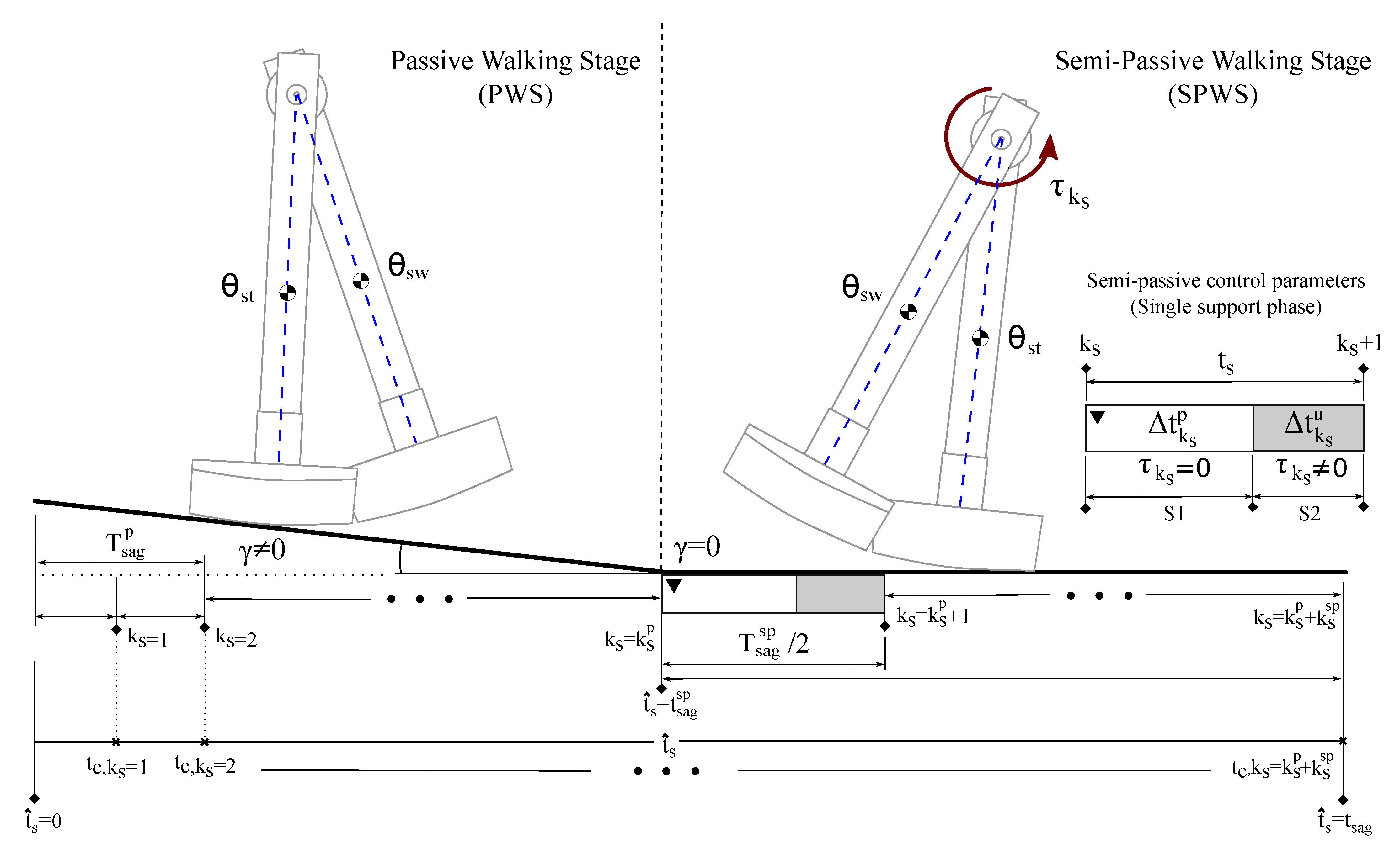
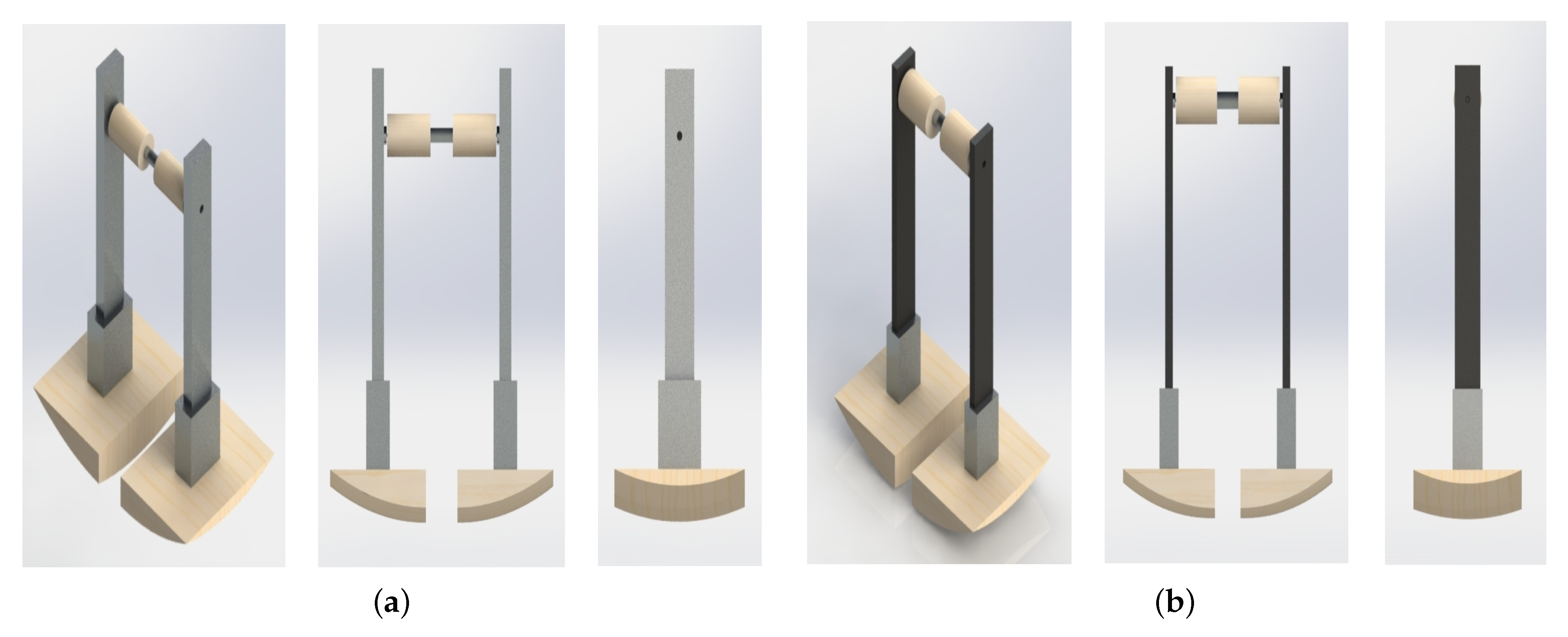
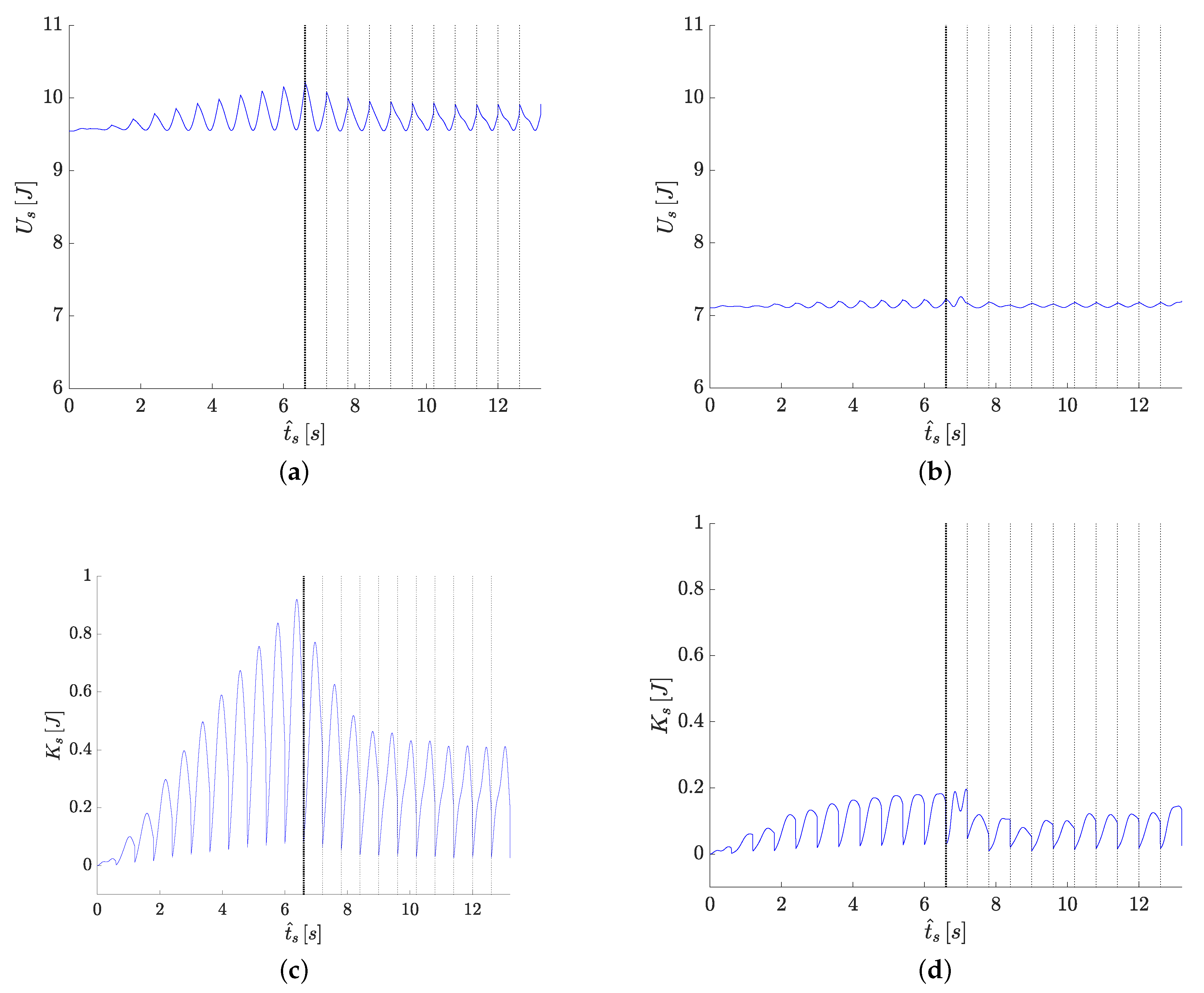
Hence, in this work, the integrated structure-control (S-C) design of a bipedal robot based on dynamic walking known as Semi-Passive Bipedal Robot (SPBR) is proposed. This approach takes advantage of the natural dynamic properties and a semi-passive control strategy to promote the convergence of the system’s dynamic behavior towards a limit cycle. The design proposal is formulated as a nonlinear discontinuous dynamic optimization problem, where the objective function is focused on achieving a periodic motion of the SPBR along with two consecutive passive (inclined ground) and semi-passive (leveled ground) walking scenarios with a minimal control effort. The considered design variables include the geometric description of each structural element, its material assignment, the control input parameters, and a set of walking conditions variables that externally modify the dynamic behavior of the SPBR. The results are validated by comparing the obtained integrated design with an SPBR derived from a sequential design process.
Due to gradient-based optimization techniques cannot efficiently handle system discontinuities, the meta-heuristic optimization method is implemented. Based on the successful use of the DE algorithm in solving integrated design problems of mechatronic systems such as in pinion-rack continuously variable transmissions [28], in five-bar parallel robots [32,33] and in digital displacement machine [34], the variant DE/rand/1/bin [35] with a constraint handling mechanism [36] is applied in the proposal with the aim of guiding the solution search towards the feasible design region. Furthermore, because the material assignment of structural elements is related to a finite set of available materials, a discrete variable handling is incorporated into the DE algorithm [37].
The rest of the paper is organized as follows: The dynamic model of the SPBR and the semi-passive control strategy are presented in Section 2. The formulation of the integrated S-C design problem is established in Section 3, where the objective function, design vector, and constraints are described. The results and a comparative analysis between the proposal and a sequential design process are presented in Section 4. Lastly, the conclusions are drawn in Section 5. The descriptions of all the used symbols in this article can be seen in Appendix A.

2. System Description

With the aim of formulating the integrated S-C design proposal, the physical implications related to the dynamic behavior of the SPBR must be established. Hence, in the following subsections, the dynamic model of the system and the proposed control strategy are presented.

2.1. SPBR Dynamic Model

To describe the dynamic behavior of the SPBR, some assumptions are defined [12]: (i) The SPBR is composed of two rigid links as legs, curved feet, and one frictionless joint placed in the hip. (ii) The motion of the SPBR takes into account frontal and sagittal plane dynamic behaviors (no walking direction changes are studied). (iii) The frontal plane dynamics is related to an oscillatory motion, which implies that the system rocks side to side for avoiding premature contact between the swing leg and the walking surface. (iv) The sagittal plane dynamics describes the stride of the system; hence, linear displacement of the SPBR is constrained to this plane. (v) The interaction between feet and walking surface neglects slipping and friction, and, the swing leg collisions are fully inelastic.
The kinematic parameters of the sagittal plane model are the foot rolling radius R s and the lengths b and d, as Figure 1. depicts. With respect to sagittal plane dynamic parameters, the system is described by the mass m s a g , the center of mass C M s a g , and the inertia moment I s a g of each leg of the SPBR. In the case of the SPBR frontal plane model, the kinematic parameters which describe the system are the length a, the separation angle ϕ , and the foot rolling radius R f , as Figure 2 shows. Moreover, the considered dynamic parameters are the mass m f r o , the link mass center C M f r o , and the inertia moment of both SPBR legs considering them as a single link.
A hybrid dynamic model describes the frontal and sagittal plane movements of the SPBR. Thus, each one of these movements is modeled by a nonlinear continuous function and a nonlinear discrete function. The nonlinear continuous function is associated with the single support phase of the bipedal gait and describes the movement of the SPBR that occurs between two consecutive collision instants k ς . Hence, in this phase, the movement is modeled from the instant when the swing leg leaves the ground (after collision instant k ς ) until the instant before it collides, and hence, a walking step finishes (before collision instant k ς + 1 ). The subscript ς f , s indicates the SPBR plane in which collision is considered, assigning ς = f and ς = s for frontal and sagittal plane, respectively. The nonlinear discrete function is related to the double support phase, which models the collision event associated with the gait cycle transition. This function describes the velocity transfer between legs when an impact happens; then, after the swing leg collides with the ground at instant k ς + 1 , the current role of each leg (determined at collision instant k ς ) is interchanged and the stance leg converts into swing leg and vice versa.

2.1.1. Single Support Phase

The dynamic response associated with the single support phase of the frontal and sagittal plane is modeled by the Euler-Lagrange method [38] and its closed form is expressed as:
M σ q η q η ¨ + C σ q η , q η ˙ q η ˙ + G σ q η   =   Φ σ t
where M σ q η is the positive semi-definite symmetric inertia matrix, C σ q η , q η ˙ is the centrifugal and Coriolis force matrix and G σ q η is the vector of gravitational forces of the SPBR. Additionally, q η q f , q s indicates the considered system states for frontal and sagittal plane, respectively, and Φ σ ( t ) is the control strategy called in this paper as semi-passive control one and is described in Section 2.1.3. The subscript σ s s , r m , f c assigns the evaluated dynamic behavior in the single support phase. In the case of the single support phase of the sagittal plane, σ = s s is assigned in (1); furthermore, the generalized coordinate vector is established as q η = s = θ s t t , θ s w t T , where the subscripts refers to the current role of the leg; thus, the subscript sw is assigned to the swing leg and the subscript st to the stance leg. With respect to the single support phase of the frontal plane, the system’s behavior is described by two dynamic conditions that depend on the angular position θ f of the SPBR. Considering Figure 2a, the first condition is presented when θ f > ϕ ; here, q η = f = θ f t and σ = r m are set in (1) to define a rolling movement caused by the foot radius R f . The second condition models the system as a fixed kinematic chain and occurs when θ f ϕ (see Figure 2b); this means that the stance leg rotates around the inner foot edge. For this second condition σ = f c is assigned in (1). For more details about single support phase model, see Appendix B of [14].

2.1.2. Double Support Phase

The swing leg collision (transition event) is described by discrete equations which relate the SPBR states just before and just after the swing leg collides with the walking surface. According to [39], the pre-impact and post-impact configurations of the system, can be determined by q η + = W q η , where W R 2 × 2 is an anti-symmetric matrix with unit elements and q η + , q η R 2 . The superscripts + and − in the system states indicate the SPBR configuration after and before collision instants, respectively. Therefore, the principle of conservation of angular momentum is used to determine the velocity transfer between both legs at collision instant k ς , ς f , s through the expression:
Ω k ς + q η q ˙ η + = Ω k ς q η q ˙ η
This equation is evaluated in the sagittal and frontal plane collisions and is only computed once per transition event. For the detailed description of the double support phase equations, see Appendix B of [14].

2.1.3. Semi-Passive Control Strategy

The proposed control strategy called semi-passive control one is focused on showing that the SPBR design can improve its walking performance by considering the passive dynamics of the system into the integrated design approach. Thus, to explore the influence of the robot’s passive properties into design tasks, the system’s dynamic behavior is tested over two consecutive walking scenarios known as Passive Walking Stage (PWS) and Semi-Passive Walking Stage (SPWS). The number of evaluated collisions determines each walking stage, assigning k s p for the collisions in the PWS and k s s p for the collisions in the SPWS. These scenarios are only defined for the sagittal plane dynamics and their evaluation is carried out along the sagittal plane walking time t ^ s , from t ^ s = 0 to t ^ s = t s a g as Figure 3 shows. In the following, both walking scenarios are explained.
First, in the PWS, the SPBR takes advantage of its structural features and gravity force to generate stable gait cycles without any control input when it is located over a surface with an inclination angle γ 0 . Thus, the passive dynamic behavior of the system is characterized by the gait cycles which occur from collision instant k s = 1 until the last collision of the PWS (i.e., k s = k s p ).
Second, in the SPWS, the surface is leveled at γ = 0 , and the control signal is suitably activated/deactivated based on a finite-state machine, which permits the system to conserve its periodic movement. This scenario evaluates the system behavior from collision instant k s = k s p + 1 until the last considered collision k s = k s p + k s s p .
Therefore, the gait characteristics derived from the PWS are used to develop gait cycles in the SPWS with regards to promoting a synergistic relationship between the structural properties and the control design features. Then, the sagittal plane dynamic behavior is associated with the gait cycle periods T s a g p and T s a g s p , both related to the periodic movements of the system in the PWS and SPWS, respectively.
On the other hand, it is assumed that the frontal plane motion is purely passive (i.e., only influenced by gravity and its initial angular position θ f i ) and is characterized by its oscillation period T f r o . It is important to remark that the single support phase time interval t s of SPWS gait cycles is determined by the half of the PWS gait period (i.e., t s = T s a g p / 2 ).
Considering that the controller is only defined along the SPWS, the finite-state machine determines the control signal mode (activated/deactivated) for each single support phase which occur in this walking scenario. There are taken into account two controller states per each single support phase time interval t s that happens after each collision instant k s . The first state S1 is related to the control signal deactivation, where the movement is only influenced by the natural dynamics of the SPBR structure; thus, along the deactivated control time interval Δ t k s p , the control input is set as Φ σ = s s t = 0 , 0 T . In the case of the second state S2, an external torque Φ σ = s s t = 0 , τ k s T , τ k s 0 is applied along the activated control time interval Δ t k s u until the single support phase finishes. Hence, the control signal is parameterized for each single support phase in the SPWS by its torque magnitude τ k s and the time interval in which the control signal is activated Δ t k s u , as can be seen in Figure 3. Moreover, the considered control signal is applied on the hip joint and only actuates the swing leg of the SPBR as is expressed in (3).
Φ σ = s s ( t ) = 0 , τ k s T if k s S P W S , t s Δ t k s u 0 , 0 T if k s P W S

3. Integrated Structure-Control Design Problem

The objective of formulating the integrated S-C design problem of the SPBR is to exploit its natural dynamic properties to find the optimal structural parameters and the activated/deactivated control signal features that assure a periodic motion along the SPWS. Thus, the PWS is implemented as a learning phase, where the obtained dynamic behavior is taken as a reference for finding the required control parameters related to the SPWS development. Therefore, the performance of the integrated S-C design approach can be benefited by assuring that the SPBR shares its passive gait characteristics along with both walking scenarios.

3.1. Objective Function

The formulation of the objective function is associated with two general design requirements. The first one is related to the walking capability of the system and implies the achievement of a synchronized periodic movement in the frontal and sagittal plane of the SPBR. In the case of the second requirement, it is proposed that the system must develop its gait cycles along the SPWS with minimum energy consumption.

3.1.1. Walking Capability Design Objective

The walking capability is related to the dynamic coupling of the frontal and sagittal plane behaviors of the SPBR. This coupling is established to promote a periodic movement that permits the gait cycle’s development. According to [14], the movement periodicity can be promoted by minimizing the differences among the system state values of consecutive transition events. Hence, the double support phases of the frontal and sagittal plane are established as Poincaré Sections to evaluate a cyclic behavior of the system along with the PWS and SPWS. Consequently, if the SPBR develops a periodic motion, its state-space trajectories must not diverge and stay close to each other. Thus, the Poincaré Map is expressed as:
q η , k ς = Q ς q η , k ς 1 η , ς f , s
where Q ς is the Poincaré Section associated with the double support phase of each SPBR plane, assigning ς = f and ς = s for the frontal and sagittal plane mappings, respectively. In (4), the system states q η of frontal and sagittal dynamic models are evaluated just after a transition happens. Then, the walking capability is promoted by minimizing the differences among the frontal and sagittal plane Poincaré mappings of the SPBR through (5). This expression evaluates the Poincaré mappings that happen in the dynamics simulation time t c of each SPBR plane.
J 1 = μ f Ψ f + μ s 1 Ψ s 1 + μ s 2 Ψ s 2
where Ψ f , Ψ s 1 and Ψ s 2 R are:
Ψ f = k f = 2 k f l a s t θ ˙ f t c , k f Q f θ ˙ f t c , k f 1 2
Ψ s 1 = k s = 2 k s p q = { s t , s w } θ q t c , k s Q s θ q t c , k s 1 2 + k s = k s p k s p + k s s p q = { s t , s w } θ q t c , k s p Q s θ q t c , k s 2
Ψ s 2 = k s = 2 k s p q = { s t , s w } θ ˙ q t c , k s Q s θ ˙ q t c , k s 1 2 + k s = k s p k s p + k s s p q = { s t , s w } θ ˙ q t c , k s p Q s θ ˙ q t c , k s 2
In (6) the differences of Poincaré mapping values associated with the frontal plane angular velocity are measured for the collision instants k f = 1 , . . . , k f l a s t which occur in the frontal plane walking time t ^ f , from t ^ f = 0 to t ^ f = t f r o . In this case, k f l a s t indicates the last collision that happens in the frontal plane walking time t ^ f . Considering that the frontal plane dynamic behavior is depicted by a back-and-forth motion, it is assumed that its transition events always occur at θ f = 0 (i.e., when both feet are instantly in contact with the ground and the symmetry axis of the SPBR is perpendicular to it). Consequently, only angular velocity is taken into account for convergence checking. In a similar manner (7) and (8) are related to the differences of angular position and angular velocity of the SPBR in the sagittal plane, respectively. In this case, both equations are divided into two terms that evaluate the Poincaré mapping values of the PWS and SPWS consecutively. Hence, to consider the passive performance of the SPBR into the SPWS, the states of all collisions that occur in the SPWS are compared to the states of the last collision of the PWS to maintain a passive influenced behavior. Additionally, the weighting factors μ f , μ s 1 and μ s 2 are established to scalarize each term of (5).

3.1.2. Energetic Efficiency Design Objective

The control effort minimization implies that the activated control time interval Δ t k s u and the torque magnitude τ k s of each single support phase of the SPWS must be the minimum for generating stable gait cycles. Therefore, the design objective related to the minimum energy consumption is expressed by (9).
J 2 = μ u 1 Ψ u 1 + μ u 2 Ψ u 2
where Ψ u 1 and Ψ u 2 R are:
Ψ u 1 = t s a g s p t s a g Φ ( t ) d t
Ψ u 2 = k s = k s p k s p + k s s p Δ t k s u
Then, the amount of torque that is provided by the control signal (3) along the SPWS is measured through (10) from the beginning of this walking scenario at t ^ s = t s a g s p until it finishes at time t ^ s = t s a g . Furthermore, the amount of time that the control signal is enabled along the SPWS is calculated by (11). For energetic efficiency design objective (9), the weighting factors μ u 1 and μ u 2 are stated.

3.1.3. General S-C Design Objective

The aggregate function describes the general S-C design objective (12), which unifies the walking capability and energetic efficiency of the SPBR as a single design objective. When the aggregate function (12) is minimized, a trade-off between the walking capability and energetic efficiency is obtained.
J = J 1 + J 2
With the aim of evaluating the general S-C design objective (12), the frontal and sagittal plane dynamic response of the SPBR must be numerically simulated. Based on [14] the dynamics simulation is carried out to evaluate the convergence of the SPBR movements and to measure the energetic requirements provided by the semi-passive control strategy. Furthermore, the existence of dynamic coupling between the frontal and sagittal plane movements is checked by calculating the oscillation periods T f r o , T s a g p and T s a g s p related to the frontal plane dynamics, the PWS and SPWS of the sagittal plane, respectively.

3.2. Design Variables

The integrated S-C design problem considers the structural parameters, the control input and a set of walking conditions of the SPBR as design domains with the aim of achieving an optimal description of the system. Consequently, the design vector p R 26 + 2 k s s p is composed by the structural design variables p s R 24 , the semi-passive control design variables p u R 2 k s s p and the walking condition variables p w c R 2 , as is expressed in (13).
p = p s , p u , p w c T
In the following subsections, the definition of each design domain variable is addressed.

3.2.1. Structural Design Variables

The structural design variables indicate the geometric description and the material assignment of the main structural elements of the SPBR. These structural elements are Foot-F, Ankle-A, Leg-L, Hip-H and Motor Case-MC. The geometric parametrization of the SPBR is shown in Figure 4 and Figure 5. Each leg of the SPBR is composed by the structural elements Foot-F, Ankle-A and Leg-L, where the part Foot-F is characterized by the subset of geometric entities R f , R s , F l , F w which depicts this element in both frontal and sagittal plane. On the other hand, the parts Ankle-A and Leg-L are described by their length-l, height-h and width-w parameters; hence, the subsets which establish their geometry are A l , A h , A w and L l , L h , L w , respectively. The joint of the SPBR is structurally determined by the elements Hip-H, Motor Case-MC and Motor-M, each per system leg. The Hip-H parameters are the radius H r , length H l and the variable H c p that describes the distance between the upper edge of the Leg-L and the axis of the joint. The Motor Case-MC is described by its length MC l and the radii MC ri and MC ro ; also, the dimensions of each lateral cover of this structural element are the length MC cl and the radius MC ro . Furthermore, the material assignment of the structural elements Foot-F, Ankle-A, Leg-L, Hip-H and Motor Case-MC is considered through their corresponding density values ρ F , ρ A , ρ L , ρ H and ρ M C , respectively. Hence, the vector of structural design variables p s R 19 is:
p s = p s g , p s m T
where p s g R 14 indicates the continuous variables related to the geometric description of the SPBR structure and p s m R 5 represents the discrete variables related to the material density of each structural element; both vectors are expressed as:
p s g = R f , R s , F l , F w , A l , A h , A w , L l , L h , L w , H l , H r , H c p , M C r o
p s m = ρ F , ρ A , ρ L , ρ H , ρ M C
Additionally, a set of constant parameters associated with the description of the structural elements Motor-M, Coupler-C, Shaft-S, and Bearing-B is established as shown in Figure 5 and Table 1. Thus, from the geometric description and material assignment of each structural element, the kinematic and dynamic model parameters of the SPBR can be determined using the procedure exposed in [14].

3.2.2. Semi-Passive Control Design Variables

With the aim of generating gait cycles in the SPWS, a control signal parametrization is carried out. This parametrization includes the torque magnitude τ k s and the activated control time interval Δ t k s u for each single support phase of the SPWS. Therefore, the vector of semi-passive control design variables p u R 2 k s s p is expressed as:
p u = p τ , p Δ t T
where p τ = τ k s p , . . . , τ k s p + k s s p R k s s p and p Δ t = Δ t k s p u , . . . , Δ t k s p + k s s p u R k s s p are vectors of torque magnitudes and activated control time intervals, respectively.

3.2.3. Walking Conditions Variables

Considering that the integrated S-C approach uses the passive dynamics of the system to influence the design performance, two physical features that externally modify the dynamic response of the SPBR are included in the design problem. For promoting an appropriate oscillatory movement in the SPBR frontal plane dynamics, its initial angular position θ f i is stated as a design variable. Additionally, the slope angle γ is considered for exploring the SPBR reconfiguration due to the influence of the passive walking dynamics along the optimization process. In the proposal, the parameter γ assigns a value that remains constant along with the entire PWS for each solution that the optimizer generates. Hence, the vector of walking condition variables p w c R 2 is established by (18).
p w c = θ f i , γ T

3.3. Constraints

The design constraints are proposed with the aim of promoting the appropriate fulfillment of both walking capability and energetic efficiency design objectives. Thus, with regards to delimiting the value of the maximum mass of the SPBR, each leg mass is constrained by (19), where m s a g , m a x = 3 kg.
g 1 : m s a g m s a g , m a x 0
As a manner of assuring geometrical pertinence of the SPBR configuration in the sagittal plane (see Figure 1), the difference between the parameters b and d must avoid negative values through the following expression (20).
g 2 : d b 0
The stance leg overturning is avoided by considering the maximum angular displacements that the SPBR develops in the frontal and sagittal planes. Hence, from Figure 4 the rolling angles β f r o and δ s a g that structurally describe the SPBR in the frontal plane and sagittal plane cannot be surpassed along with the development of both walking scenarios. The frontal and sagittal plane rolling angles are determined in (21) and (22), respectively.
β f r o = arcsin F l + F ϕ R f + ϕ
δ s a g = arcsin F w R s
where:
F ϕ = H l + 2 M C c l + M C l + C w + 1 2 L l F l
Consequently the constraints of maximum angular displacements (24) and (25) are established, where m a x θ f t and m a x θ s t t , θ s w t are values which vary depending on the kinematic and dynamic features of each solution that are provided by the optimizer. Hence, from a set of design variable values, these parameters are determined through simulating frontal and sagittal plane dynamic models of the system.
g 3 : m a x θ f t β f r o 0
g 4 : m a x θ s t t , θ s w t δ s a g 0
According to the SPBR model assumptions, a dynamic coupling between the frontal and sagittal planes must exist to generate stable gait cycles along both walking stages. Hence, the value of frontal plane oscillation period must be initially bounded to a feasible gait period through the expressions (26) and (27), where T i n f = 0.6 s and T s u p = 1.6 s .
g 5 : T i n f T f r o 0
g 6 : T f r o T s u p 0
Then, it is assumed that T s a g p and T s a g s p oscillation periods, which correspond to the PWS and SPWS of the sagittal plane, respectively, must coincide with the frontal plane oscillation period T f r o . Therefore, the conditions (28) and (29) are established to achieve a dynamic coupling between the frontal plane motion and the gait period of each walking stage of the sagittal plane. In these expressions, ϵ = 0.001 is established as a constant tolerance value.
g 7 : T f r o T s a g p ϵ 0
g 8 : T f r o T s a g s p ϵ 0
The SPBR structural design is also constrained by the upper and lower bounds of the geometric design variables through (30) and (31), where the maximum and minimum values of each geometric structural variable are established in Table 2.
g 9 : p s g p s g , m a x 0
g 10 : p s g , m i n p s g 0
Moreover, the material assignment of the structural elements Foot-F, Ankle-A, Leg-L, Motor Case-MC and Hip-H is carried out by taking into account a set of discrete values related to the available material densities as (32) establishes. The selected materials are Medium Density Fibreboard (MDF), Polylactic Acid (PLA plastic) and Aluminum, where their density values are ρ M D F = 450 kg/m 3 , ρ P L A = 1250 kg/m 3 and ρ A L = 2700 kg/m 3 respectively.
p s m ρ M D F , ρ P L A , ρ A L
In the case of semi-passive control design variables, the torque magnitudes are limited through the expressions (33) and (34). The upper and lower torque values are p τ , m a x = 1.5 N m · 1 and p τ , m i n = 0 , where 1 R k s s p and 0 R k s s p are vectors with elements set as one and zero, respectively.
g 11 : p τ p τ , m a x 0
g 12 : p τ , m i n p τ 0
Moreover, the activated control time intervals are delimited by (35) and (36). The upper and lower limits of activated control time intervals are p Δ t , m a x = T f r o / 2 s · 1 and p Δ t , m i n = 0 . Hence, the upper limit depends on the dynamic behavior of each solution provided by the optimizer.
g 13 : p Δ t p Δ t , m a x 0
g 14 : p Δ t , m i n p Δ t 0
Finally, the limits of the walking condition variables are expressed in (37) and (38), where the bounding values are enlisted in Table 3.
g 15 : p w c p w c , m a x 0
g 16 : p w c , m i n p w c 0

3.4. Optimization Problem Formulation

The integrated S-C design of the SPBR is formulated as a nonlinear discontinuous dynamic optimization problem with mixed design variables. It consists of finding the optimal design vector p (13) that establishes the geometric description and material assignment of the SPBR structural components, the parameters of the semi-passive control strategy for each single support phase that occurs in the SPWS, the inclination of the ground in the PWS and the initial condition in the frontal plane which simultaneously minimizes the differences among the Poincaré mapping values of consecutive gait cycles (5) and its energetic requirements (9) through promoting a passive influenced dynamic behavior of the system along with both walking scenarios, i.e., the minimization is in the aggregate function J (12). Thus, the formulation of the optimization problem is stated as follows:
M i n p J
subject to:
  • The dynamic model of the system (1) and (2).
  • The design and operating requirements of the SPBR (19), (20), (24)–(27).
  • The dynamic coupling conditions (28) and (29).
  • The limits of the structural geometric variables and the available materials (30)–(32).
  • The limits of the semi-passive control parameters (33)–(36).
  • The limits of the walking conditions variables (37) and (38).

4. Results and Discussion

In this Section, the proposed integrated S-C design results are presented in two parts: First, the solution search performance of the integrated design proposal is addressed by evaluating a set of DE algorithm executions; here, the evolution of the best population along the optimization process is shown. Second, the best solution of the integrated S-C design is compared with the best one associated with a sequential design procedure. In this case, the walking performance and semi-passive control features of the best solution per each design process are studied.

4.1. Integrated S-C Design

The integrated design problem is solved by the DE algorithm variant DE/rand/1/bin through considering the following algorithm parameters: a population size of N P = 80 individuals and stop criterion G m a x = 6000 are established; the scale factor F and crossover factor C R are randomly assigned at each generation of the optimization process, where the former is taken from the interval 0.3 F 0.9 and the latter from 0.8 C R 1 . The values of the weighting factors are set by a trial and error procedure as μ f = 1000 , μ s 1 = 15 , μ s 2 = 15 , μ u 1 = 0.01 and μ u 2 = 7 . With respect to the simulation of the SPBR dynamics, frontal plane behavior is evaluated for a simulation time t f r o = 10 s ; also, the initial conditions θ f , θ ˙ f T = θ f i , 0 T are taken into account. Sagittal plane simulation is carried out for both consecutive walking stages, where the PWS is evaluated for k s p = 10 collisions and the SPWS for k s s p = 11 collisions; in addition, the vector of initial conditions θ s t , θ s w , θ ˙ s t , θ ˙ s w T = 0 , 0 , 0 , 0 T is considered for sagittal plane dynamics simulation.
Ten independent runs of the optimization algorithm are performed using a PC with a 2.5 GHz Intel Core(TM) i5 processor and 8GB of RAM. The DE algorithm for the solution of the integrated S-C design problem is programmed in MATLAB©. The mean convergence time of the DE algorithm for runs is around three hours. The minimum values of the aggregate function J ( p ) , the walking capability J 1 ( p ) and energetic efficiency J 2 ( p ) design objectives per each DE run are presented in Table 4. Additionally, the standard deviation (S.D.) related to the aggregate function of the last population individuals of each run are shown in Table 4. As observed, minimization of design objectives converges towards the same region of the objective space at each algorithm execution; this fact is determined by the values of standard deviation, which imply not scattered solutions. Moreover, all algorithm runs achieve feasible populations. Therefore, whatever solution in Table 4 can be an option in the proposed structure-control design approach, but the best is selected to compare with the sequential design approach in Section 4.2.
With respect to the solution search convergence, Figure 6a show how the mean of the aggregate function J m e a n of the best population evolves along the optimization process, whereas Figure 6b depicts the behavior of the mean of violated constraint values V C m e a n . Then, as denoted by the dashed line in Figure 6, the population individuals become all feasible solutions at G = 1325 (i.e., all the constraints are satisfied for each individual provided by the optimizer). The structural and walking condition variables of the best solution are presented in Table 5; additionally, the values of its semi-passive control design variables are shown in Table 6.

4.2. Integrated Structure-Control Design versus Sequential Design

To evaluate the performance of the integrated design results, a sequential design process is carried out. Hence, the best solution of the S-C design is compared with the best of the sequential one.
Sequential design process consists of two design stages that address structural and control design in a separate manner. For the study case, structural design is made according to [14], where the optimal structural design of a passive bipedal walker is developed through considering a dynamic coupling between frontal and sagittal plane dynamic behaviors of the system. Then, this structural design process is carried out for obtaining a reference of passive walking behavior, evaluating the SPBR dynamics without any control input. Therefore, the structural parameters are obtained through minimizing (6) and the first term of (7) and (8), which are related to the PWS, for the design vector p ^ s = p s g , p s m , p w c T and subject to the constraints (19), (20), (24)–(28), (30)–(32), (37) and (38). In this design stage, the weighting factors of (6)–(8) are suitably set according to [14] with the purpose of assuring an appropriate dynamic coupling between frontal and sagittal plane (i.e., passive walking capability is fulfilled). The system’s simulation considers the same parameters and initial conditions as integrated S-C design process. Consequently, the result of this structural design must describe a passive bipedal walker that accomplishes a dynamic coupling between its frontal and sagittal plane behaviors.
Once structural design process is performed, the semi-passive control parameters for the best solution of this design phase can be determined as integrated S-C design approach indicates in Section 2.1.3 and Section 3. Then, the control input parameters are obtained by testing the SPBR’s structure along the PWS and SPWS to minimize the aggregate function (12) for the design vector p ^ u = p τ , p Δ t T and subject to the constraints (25), (29) and (33)–(36). It is important to remark that DE/rand/1/bin is also implemented for solving each stage of sequential design. Moreover, algorithm parameters F, C R and N P are stated as in the integrated case; the stop criterion G m a x = 3000 is established for each sequential design stage.
Structural and walking condition variables of the best designs for both approaches are enlisted in Table 5. Additionally, their dynamic model parameters are presented in Table 7. The frontal and sagittal plane dynamic behaviors of integrated and sequential solutions are depicted in Figure 7, where a dashed line depicts the limit cycle of the PWS for both designs in Figure 7c,d, respectively; meanwhile, SPWS gait cycle trajectories are shown by solid lines also in Figure 7c,d. Through considering the same weighting factors as the integrated design approach, in Table 8 the differences of angular displacements and velocities along with frontal and sagittal plane dynamics simulation, in addition to the amount of torque and activated control time of the best solution of sequential design are used to calculate its value of the aggregate function and design objectives. Then, a comparison among aggregate function, walking capability and energetic efficiency of both S-C and sequential design is addressed in columns J ( p ) , J 1 ( p ) and J 2 ( p ) of Table 8, respectively. The features of angular movements of the frontal and sagittal plane of the SPBR related to integrated S-C and sequential design are exposed in Table 9.
To address the influence of the semi-passive control strategy into both design approaches, the angular displacements of the left θ l e f t and right θ r i g h t leg of the SPBR along sagittal plane simulation time t ^ s are plotted in Figure 8a,b; thick trajectories in the SPWS are related to the single support phases that are influenced by the semi-passive control signal (swing leg displacement of the current gait cycle). Furthermore, the semi-passive control activations are shown in Figure 8c,d, where the control signal parameters are presented in Table 6. In each plot of Figure 8, the dotted vertical lines indicate the collision instants of each single support phase of the SPWS. The structural description of each obtained design is shown in Figure 9, where the CAD rendering of both designs is presented.
Thus, according to Table 5 and Table 6 and Figure 7 and Figure 8, the following findings are observed:
  • Integrated S-C design obtains a better synergy between walking capability and energetic efficiency design objectives than the sequential design method. This is demonstrated by assuming that a better synergy between criteria is when the trade-off in the aggregate function J ( p ) is minimum, meaning that waking capability and energetic efficiency are in equilibrium, the proposal reduces around 63.55 % the value of the aggregate function J ( p ) with respect to the sequential design (based on the column J ( p ) of Table 8). The overall behavior of both designs is shown in Figure 8. Both designs can develop a gait cycle in the two walking stages, i.e., the walking capability J 1 ( p ) is suitable in both designs. Nevertheless, the proposal reduces 95.41 % of the control activation and its magnitude with respect to the sequential design based on the values reported in the column J 2 ( p ) of Table 8.
  • In both design approaches, the proposed semi-passive control strategy can produce a periodic movement of the SPBR into the SPWS. This achieves the same dynamic coupling between the frontal plane movement and the gait periods in both the PWS and SPWS of the sagittal plane (the dynamic coupling is reached in the oscillation periods T f r o = T s a g p = T s a g s p = 1.2 s , as indicates in Table 7). Thus, the walking capability for integrated and sequential design is assured.
  • The semi-passive control signal is activated around 5% of the SPWS time in the integrated design (see Table 6 and Figure 8c). Meanwhile, in the sequential design, the semi-passive control strategy is activated around 89 % of the SPWS time (see Figure 8d). The features of the achieved semi-passive control signal in the integrated design are attributed to the high amplitude of the potential and kinetic energies oscillation (see Figure 10). This contributes to keeping the dynamic response of the SPBR into the corresponding limit cycle for a long time without the control influence. Hence, this results in the reduction of the control system activation.
  • Based on the structure of the SPBR, the center of mass of integrated and sequential design is located almost at the same height with respect to the leveled ground (see columns C M f r o y and C M s a g y of Table 7). Nevertheless, the value of mass related to the integrated design is higher in comparison with the sequential one. In addition, it is observed that integrated S-C design approach exploit the structural properties of the SPBR to promote higher angular displacements along the PWS and SPWS. This fact is shown in Table 9, where the ratio between the maximum angular displacements and the permitted rolling angles in frontal and sagittal plane of the SPBR are m a x θ f t 0.81 β f r o and m a x θ s t t , θ s w t 0.98 δ s a g , respectively. Meanwhile, for the sequential design these relationships are m a x θ f t 0.33 β f r o and m a x θ s t t , θ s w t 0.88 δ s a g , respectively. Furthermore, the amplitude of the movement in frontal plane of the S-C design is associated with the value of R f and θ f i , where in both cases, integrated design approach provides higher values for these design variables. With respect to the sagittal plane, although the best design of each approach converged towards the same value of inclination angle γ in the PWS, the structure and control parameters of the integrated one induced that the angular displacement and velocity are higher in both walking scenarios in comparison with the sequential design (see Table 9 and Figure 7). Therefore, the natural dynamics of the SPBR structure promotes a suitable recovery between the kinetic and potential energy to maintain the limit cycle with minimum control effort.

5. Conclusions

In this work, the design of a SPBR that simultaneously considers structural (geometrical and material configuration) and control parameters (torque magnitudes and activated control time intervals) is proposed as an integrated S-C design approach. A nonlinear discontinuous dynamic optimization problem with mixed design variables is formulated by taking into account the walking capability and energy consumption of the SPBR. The natural dynamic properties of the system are included in the design tasks by establishing two consecutive walking scenarios and a semi-passive control strategy.
A comparison between the proposal and a sequential design process indicates that the proposal reduces around 63.55 % the value of the performance function related to the synergy between the walking capability and energetic efficiency with respect to the sequential design. Despite both designs can develop gait cycle in the two walking stages, i.e., the dynamic coupling is achieved for the frontal and sagittal plane, the proposal reduces 95.41 % of the control activation and its magnitude with respect to the sequential design meaning a decrement in the energy consumption. It is also observed that the structural parameters that greatly influence the integrated design performance are related to the initial condition of the frontal plane, the feet curvature radii, the mass, and the angular displacement amplitude of the SPBR, promoting a better walking capability and a reduction of the energy consumption. This can be attributed to the natural dynamics of the SPBR structure developing a suitable recovery between the kinetic and potential energy to maintain the limit cycle with minimum control effort. The proposal results emphasize that the different structure and control reconfigurability based on the natural dynamics of a mechatronic system can significantly influence the overall system performance.
The proposed integrated S-C design approach assumes that there are no uncertainties in the optimization problem formulation. Hence, future research direction involves the robust integrated structure-control design for bipedal robots based on passive dynamic walking to handle uncertainties in the problem formulation.

Author Contributions

Conceptualization, methodology, formal analysis, investigation, writing—review and editing, visualization, M.G.V.-C. and J.N.M.-C.; data curation, software, validation, writing—original draft preparation, J.N.M.-C.; resources, supervision, project administration, funding acquisition, M.G.V.-C. All authors have read and agreed to the published version of the manuscript.

Funding

This work was funded in part by the economic support program of the Comisión de Operación y Fomento de Actividades Académicas (COFAA) and the Secretaría de Investigación y Posgrado (SIP) of the Instituto Politécnico Nacional under Grant 20180196, 20190239 and 20210374.

Institutional Review Board Statement

Not applicable.

Informed Consent Statement

Not applicable.

Data Availability Statement

Data are available on request from the corresponding author.

Acknowledgments

The authors acknowledge the support from the COFAA and the Secretaría de Investigación y Posgrado (SIP) of the Instituto Politécnico Nacional, and CONACYT. The first author acknowledges the support from the Consejo Nacional de Ciencia y Tecnología (CONACyT) in Mexico through a scholarship to pursue graduate studies at CIDETEC-IPN.

Conflicts of Interest

The authors declare no conflict of interest.

Appendix A. Nomenclature

With the aim of present the used nomenclature, the symbols have been classified into two main areas: SPBR dynamic model symbols (Table A1) and integrated S-C design problem symbols (Table A2). The header of each subgroup of symbols denotes the ambit where the symbols are mainly considered.
Table A1. SPBR dynamic model symbols.
SymbolDefinition
General
SPBRSemi-Passive Bipedal Robot
S-CStructure-control design
PWSPassive Walking Stage
SPWSSemi-Passive Walking Stage
M σ Inertia matrix
C σ Centrifugal and Coriolis matrix
G σ Gravity forces vector
η f , s Generalized coordinates assignment
σ s s , r m , f c SPBR behavior assignment
ς f , s SPBR plane assignment
gAcceleration due to gravity
Sagittal plane [14]
m s a g Mass of SPBR leg
I s a g Inertia moment of SPBR leg
R s Foot radius
bDistance between leg mass center and the center of R s
dDistance between hip and the center of R s
γ Slope angle
θ s t , θ ˙ s t Angular position and velocity of stance leg
θ s w , θ ˙ s w Angular position and velocity of swing leg
T s a g p , T s a g s p Sagittal plane gait period (PWS and SPWS)
Ω , Ω + Pre-impact and post-impact angular momentum matrices
s s Single support phase of sagittal plane
δ s a g Foot rolling angle
Frontal plane [14]
m f r o Total mass of the SPBR
I f r o Inertia moment of the SPBR
R f Foot radius
aDistance between mass center and the center of R f
ϕ Half of feet separation angle
θ f , θ ˙ f Angular position and velocity of the SPBR
T f r o Oscillation period
θ f ˙ , θ f ˙ + Angular velocity before and after collision event
r m Foot rolling movement
f c Fixed kinematic chain behavior
β f r o Foot rolling angle
Table A2. Integrated S-C design problem symbols.
SymbolDefinition
Parametrization
pDesign vector
p s Vector of structure design variables
p s g Vector of geometric design variables
p s m Vector of material assignment variables
p u Vector of semi-passive control design variables
p τ Vector of torque magnitudes
p Δ t Vector of activated control time intervals
p w c Vector of walking condition variables
τ k s Torque magnitude
Δ t k s u Activated control time interval
F l , F h , F w , R s , R f Foot-F geometric parameters
A l , A h , A w Ankle-A geometric parameters
L l , L h , L w Leg-L geometric parameters
H l , H r , H c p Hip-H geometric parameters
M C r o , M C r i , M C l , M C c l Motor Case-MC geometric parameters
B r o , B r i , B w Bearing-B geometric parameters
C r o , C r i , C w Coupler-C geometric parameters
ρ F , ρ A , ρ L , ρ H , ρ M C Foot-F, Ankle-A, Leg-L, Hip-H and Motor Case-MC densities
θ f i Initial condition of frontal plane simulation
Optimization problem
JAggregate function
J 1 Walking capability design objective
J 2 Energetic efficiency design objective
Ψ f Difference of Poincaré mapping values ( θ ˙ f )
Ψ s 1 Difference of Poincaré mapping values ( θ q )
Ψ s 2 Difference of Poincaré mapping values ( θ ˙ q )
Ψ u 1 Measure of torque along SPWS
Ψ u 2 Measure of activated control time along SPWS
μ f , μ s 1 , μ s 2 , μ u 1 , μ u 2 Aggregate function weights
Q ς Poincaré Map
t c Collision instant time
k f Collision counter of frontal plane
k s Collision counter of sagittal plane
t f r o , t s a g Frontal and sagittal dynamics simulation time
Differential algorithm
G m a x Maximum number of generations (stop criterion)
N P Population size
C R Crossover factor
K,FScale factors

References

  1. Westervelt, E.R.; Grizzle, J.W.; Chevallereau, C.; Choi, J.H.; Morris, B. Feedback Control of Dynamic Bipedal Robot Locomotion; CRC Press: Boca Raton, FL, USA, 2007; Volume 28. [Google Scholar]
  2. Wisse, M. Essentials of Dynamic Walking; Analysis and Design of Two-Legged Robots. Ph.D. Thesis, Delft University of Technology, Delft, The Netherlands, September 2004. [Google Scholar]
  3. Sakagami, Y.; Watanabe, R.; Aoyama, C.; Matsunaga, S.; Higaki, N.; Fujimura, K. The intelligent ASIMO: System overview and integration. In Proceedings of the IEEE/RSJ International Conference on Intelligent Robots and Systems, Lausanne, Switzerland, 30 September–4 October 2002; Volume 3, pp. 2478–2483. [Google Scholar]
  4. Kaneko, K.; Harada, K.; Kanehiro, F.; Miyamori, G.; Akachi, K. Humanoid robot HRP-3. In Proceedings of the 2008 IEEE/RSJ International Conference on Intelligent Robots and Systems, Nice, France, 22–26 September 2008; pp. 2471–2478. [Google Scholar]
  5. Stasse, O.; Verrelst, B.; Vanderborght, B.; Yokoi, K. Strategies for humanoid robots to dynamically walk over large obstacles. IEEE Trans. Robot. 2009, 25, 960–967. [Google Scholar] [CrossRef]
  6. Collins, S.; Ruina, A.; Tedrake, R.; Wisse, M. Efficient bipedal robots based on passive-dynamic walkers. Science 2005, 307, 1082–1085. [Google Scholar] [CrossRef] [PubMed] [Green Version]
  7. McGeer, T. Passive dynamic walking. J. Robot. Res. 1990, 9, 62–82. [Google Scholar] [CrossRef]
  8. Wisse, M.; Keliksdal, G.; Van Frankenhyyzen, J.; Moyer, B. Passive-based walking robot. IEEE Robot. Autom. Mag. 2007, 14, 52–62. [Google Scholar] [CrossRef]
  9. Collins, S.H.; Ruina, A. A bipedal walking robot with efficient and human-like gait. In Proceedings of the 2005 IEEE International Conference on Robotics and Automation, Barcelona, Spain, 18–22 April 2005; pp. 1983–1988. [Google Scholar]
  10. Ebrahimi, A.; Heydari, M.; Alasty, A. Active control of a passive bipedal walking robot. Int. J. Dyn. Control 2017, 5, 733–740. [Google Scholar] [CrossRef]
  11. Kajita, S.; Yamaura, T.; Kobayashi, A. Dynamic walking control of a biped robot along a potential energy conserving orbit. IEEE Trans. Robot. Autom. 1992, 8, 431–438. [Google Scholar] [CrossRef]
  12. Tedrake, R.; Zhang, T.W.; Fong, M.F.; Seung, H.S. Actuating a simple 3D passive dynamic walker. In Proceedings of the IEEE International Conference on Robotics and Automation, New Orleans, LA, USA, 26 April–1 May 2004; Volume 5, pp. 4656–4661. [Google Scholar]
  13. Bhounsule, P.A.; Cortell, J.; Grewal, A.; Hendriksen, B.; Karssen, J.D.; Paul, C.; Ruina, A. Low-bandwidth reflex-based control for lower power walking: 65 km on a single battery charge. Int. J. Robot. Res. 2014, 33, 1305–1321. [Google Scholar] [CrossRef]
  14. Martínez-Castelán, J.N.; Villarreal-Cervantes, M.G. Frontal-Sagittal Dynamic Coupling in the Optimal Design of a Passive Bipedal Walker. IEEE Access 2018, 1. [Google Scholar] [CrossRef]
  15. Pantoja-García, J.S.; Villarreal-Cervantes, M.G.; García-Mendoza, C.V.; Silva-García, V.M. Synergistic Design of the Bipedal Lower-Limb through Multiobjective Differential Evolution Algorithm. Math. Probl. Eng. 2019, 2019, 2301714. [Google Scholar] [CrossRef]
  16. Villarreal-Cervantes, M.G.; Pantoja-García, J.S.; Rodríguez-Molina, A.; Benitez-Garcia, S.E. Pareto optimal synthesis of eight-bar mechanism using meta-heuristic multi-objective search approaches: Application to bipedal gait generation. Int. J. Syst. Sci. 2021, 52, 671–693. [Google Scholar] [CrossRef]
  17. Tsuge, B.Y.; Plecnik, M.M.; McCarthy, J.M. Homotopy directed optimization to design a six-bar linkage for a lower limb with a natural ankle trajectory. J. Mech. Robot. 2016, 8, 061009. [Google Scholar] [CrossRef] [Green Version]
  18. Huang, Y.; Wang, Q.; Xie, G.; Wang, L. Optimal mass distribution for a passive dynamic biped with upper body considering speed, efficiency and stability. In Proceedings of the Humanoids 2008—8th IEEE-RAS International Conference on Humanoid Robots, Daejeon, Korea, 1–3 December 2008; pp. 515–520. [Google Scholar]
  19. Hale, A.L.; Dahl, W.; Lisowski, J. Optimal simultaneous structural and control design of maneuvering flexible spacecraft. J. Guid. Control. Dyn. 1985, 8, 86–93. [Google Scholar] [CrossRef]
  20. Asada, H.; Park, J.H.; Rai, S. A control-configured flexible arm: Integrated structure control design. In Proceedings of the Robotics and Automation, Sacramento, CA, USA, 9–11 April 1991; pp. 2356–2362. [Google Scholar]
  21. Zhang, Y.; Yang, D.; Li, S. An integrated control and structural design approach for mesh reflector deployable space antennas. Mechatronics 2016, 35, 71–81. [Google Scholar] [CrossRef]
  22. Bastos, G. A Synergistic Optimal Design for Trajectory Tracking of Underactuated Manipulators. J. Dyn. Syst. Meas. Control 2019, 141, 021015. [Google Scholar] [CrossRef]
  23. Sands, T. Optimization Provenance of Whiplash Compensation for Flexible Space Robotics. Aerospace 2019, 6, 93. [Google Scholar] [CrossRef] [Green Version]
  24. Biegler, L.T. An overview of simultaneous strategies for dynamic optimization. Chem. Eng. Process. Process Intensif. 2007, 46, 1043–1053. [Google Scholar] [CrossRef]
  25. Paul, C.; Bongard, J.C. The road less travelled: Morphology in the optimization of biped robot locomotion. In Proceedings of the 2001 IEEE/RSJ International Conference on Intelligent Robots and Systems, Maui, HI, USA, 29 October–3 November 2001; Volume 1, pp. 226–232. [Google Scholar]
  26. Matsushita, K.; Yokoi, H.; Arai, T. Pseudo-passive dynamic walkers designed by coupled evolution of the controller and morphology. Robot. Auton. Syst. 2006, 54, 674–685. [Google Scholar] [CrossRef]
  27. Ravichandran, T.; Wang, D.; Heppler, G. Simultaneous plant-controller design optimization of a two-link planar manipulator. Mechatronics 2006, 16, 233–242. [Google Scholar] [CrossRef]
  28. Portilla-Flores, E.A.; Mezura-Montes, E.; Álvarez-Gallegos, J.; Coello-Coello, C.A.; Cruz-Villar, C.A. Integration of structure and control using an evolutionary approach: An application to the optimal concurrent design of a CVT. Int. J. Numer. Methods Eng. 2007, 71, 883–901. [Google Scholar] [CrossRef]
  29. Villarreal-Cervantes, M.G.; Cruz-Villar, C.A.; Alvarez-Gallegos, J.; Portilla-Flores, E.A. Robust structure-control design approach for mechatronic systems. IEEE/ASME Trans. Mechatron. 2013, 18, 1592–1601. [Google Scholar] [CrossRef]
  30. Valdez, S.I.; Chávez-Conde, E.; Hernandez, E.E.; Ceccarelli, M. Structure-control design of a mechatronic system with parallelogram mechanism using an estimation of distribution algorithm. Mech. Based Des. Struct. Mach. 2016, 44, 58–71. [Google Scholar] [CrossRef]
  31. Villarreal-Cervantes, M.G. Approximate and widespread Pareto solutions in the structure-control design of mechatronic systems. J. Optim. Theory Appl. 2017, 173, 628–657. [Google Scholar] [CrossRef]
  32. Villarreal-Cervantes, M.G.; Cruz-Villar, C.A.; Alvarez-Gallegos, J.; Portilla-Flores, E.A. Differential evolution techniques for the structure-control design of a five-bar parallel robot. Eng. Optim. 2010, 42, 535–565. [Google Scholar] [CrossRef]
  33. Cervantes-Culebro, H.; Cruz-Villar, C.A.; Peñaloza, M.G.M.; Mezura-Montes, E. Constraint-Handling Techniques for the Concurrent Design of a Five-Bar Parallel Robot. IEEE Access 2017, 5, 23010–23021. [Google Scholar] [CrossRef]
  34. Bech, M.M.; Noergaard, C.; Roemer, D.B.; Kukkonen, S. A global multi-objective optimization tool for design of mechatronic components using Generalized Differential Evolution. In Proceedings of the IECON 2016—42nd Annual Conference of the IEEE Industrial Electronics Society, Florence, Italy, 23–26 October 2016; pp. 475–481. [Google Scholar] [CrossRef]
  35. Storn, R.; Price, K. Differential evolution–a simple and efficient heuristic for global optimization over continuous spaces. J. Glob. Optim. 1997, 11, 341–359. [Google Scholar] [CrossRef]
  36. Mezura-Montes, E.; Coello, C.A.C. Constraint-handling in nature-inspired numerical optimization: Past, present and future. Swarm Evol. Comput. 2011, 1, 173–194. [Google Scholar] [CrossRef]
  37. Lampinen, J.; Zelinka, I. Mixed integer-discrete-continuous optimization by differential evolution, Part 1: The optimization method. In Proceedings of the 5th International Conference on Soft Computing, Brno, Czech Republic, 9–12 June 1999; pp. 71–76. [Google Scholar]
  38. Spong, M.W.; Hutchinson, S.; Vidyasagar, M. Robot Modeling and Control; Wiley: New York, NY, USA, 2006; Volume 3. [Google Scholar]
  39. Goswami, A.; Thuilot, B.; Espiau, B. A study of the passive gait of a compass-like biped robot: Symmetry and chaos. Int. J. Robot. Res. 1998, 17, 1282–1301. [Google Scholar] [CrossRef]
Figure 1. Sagittal plane configuration of SPBR in single support phase.
Mathematics 09 01482 g001
Figure 2. Frontal plane configuration of SPBR in single support phase.
Mathematics 09 01482 g002
Figure 3. Walking stages of SPBR.
Mathematics 09 01482 g003
Figure 4. Schematic diagram of the SPBR.
Mathematics 09 01482 g004
Figure 5. Structural element parametrization. The label * is assigned for constant geometric values. Additionally, the notation FV = Frontal View and LV = Lateral View is considered.
Mathematics 09 01482 g005
Figure 6. Evolution of the best S-C design execution: (a) Convergence of the mean value of the aggregate function J m e a n . (b) Convergence of the mean value of the violated constraints V C m e a n .
Mathematics 09 01482 g006
Figure 7. Dynamic behavior of the best solutions of S-C and sequential design processes. Limit cycle of frontal plane dynamics: (a) S-C design. (b) Sequential design. PWS and SPWS limit cycles of the sagittal plane (right leg of SPBR): (c) S-C design. (d) Sequential design.
Mathematics 09 01482 g007
Figure 8. Angular displacements of the left θ l e f t and right θ r i g h t leg of the SPBR along with the PWS and SPWS: (a) S-C design. (b) Sequential design. Activation/Deactivation of the semi-passive control signal: (c) S-C design. (d) Sequential design.
Mathematics 09 01482 g008
Figure 9. CAD representation of the SPBR: (a) S-C design. (b) Sequential design.
Mathematics 09 01482 g009
Figure 10. Behavior of the SPBR mechanical energy along the PWS and SPWS. Potential energy U s : (a) S-C design. (b) Sequential design. Kinetic energy K s : (c) S-C design. (d) Sequential design.
Mathematics 09 01482 g010
Table 1. Constant parameters of structural elements.
Structural ElementParameterValue
Motor-M m M (kg)0.1060
M b l (m)0.0747
M b r (m)0.0125
M s l (m)0.0125
M s r (m)0.0020
Coupler-C m C (kg)0.0037
C r o (m)0.0095
C r i (m)0.0020
C w (m)0.0050
Bearing-B m B (kg)0.0054
B r o (m)0.0065
B r i (m)0.0050
B w (m)0.0126
Shaft-S m S (kg)0.0150
S r (m)0.0055
S l (m)0.0200
Table 2. Upper and lower bounds of geometric design variables p s g .
Variable p max p min
R f (m)0.700
R s (m)0.700
F l (m)0.150
F w (m)0.150
A l (m)0.050.02
A h (m)0.060.02
A w (m)0.080.04
L l (m)0.050.015
L h (m)0.500
L w (m)0.080.04
H l (m)0.20.02
H r (m)0.060.0075
H c p (m)0.300.04
M C r o (m)0.060.02
Table 3. Upper and lower bounds of walking condition variables p w c .
Variable p wc , max p wc , min
θ f i (rad)0.3830.174
γ (rad)0.1390.034
Table 4. The best results of each algorithm execution. The solution marked in boldface represents the best among runs.
Run J ( p ) J 1 ( p ) J 2 ( p ) S.D.
120.111017.83442.27660.1791
219.759417.23782.52160.1915
319.942614.72185.22070.1586
419.670314.52135.14890.2091
522.431816.40626.02550.3124
619.048616.87702.17150.0938
717.841515.94991.89150.2100
822.078815.24836.83050.0260
920.003717.86712.13650.0261
1021.053615.06295.99060.0617
Table 5. Optimal structure and walking condition design variables associated with the best solution obtained by structure-control (S-C) and sequential (Seq.) design processes.
p VariableS-C/Seq.
p s g R f (m)0.4266/0.3563
R s (m)0.4731/0.5493
F l (m)0.1784/0.1800
F w (m)0.1195/0.1154
A l (m)0.0439/0.0374
A h (m)0.0915/0.0998
A w (m)0.0786/0.0636
L l (m)0.0222/0.0150
L h (m)0.3207/0.3994
L w (m)0.0535/0.0543
H l (m)0.0208/0.0200
H r (m)0.0076/0.0109
H c p (m)0.0690/0.0423
M C r o (m)0.0221/0.0295
p s m ρ F (kg/m 3 )450/450
ρ A (kg/m 3 )2700/2700
ρ L (kg/m 3 )2700/1250
ρ H (kg/m 3 )2700/2700
ρ M C (kg/m 3 )450/450
p w c θ f i r a d 0.3577/0.1782
γ r a d 0.0262/0.0262
Table 6. Optimal semi-passive control design variables associated with the best solutions obtained by structure-control (S-C) and sequential (Seq.) design processes.
Δ t k s u ( s ) τ k s ( Nm )
k s = k s p + i S-C/Seq.S-C/Seq.
i = 1 0.0890/0.49140.8271/0.3777
i = 2 0.0034/0.34510.6365/0.1699
i = 3 0.0177/0.46210.9904/0.2288
i = 4 0.1039/0.57460.4626/0.3034
i = 5 0.0080/0.52380.2880/0.3243
i = 6 0.0112/0.56100.4088/0.3798
i = 7 0.0033/0.57410.4450/0.3896
i = 8 0.0181/0.59780.3761/0.3478
i = 9 0.0183/0.57270.1880/0.4162
i = 10 0.0061/0.59670.3825/0.3618
i = 11 0.0094/0.58390.0397/0.5712
Table 7. Dynamic model parameters of the best solutions obtained by structure-control (S-C) and sequential (Seq.) design processes.
Sagittal plane parameters
m s a g (kg) I s a g ( kg m 3 ) b ( m ) d ( m ) C M s a g y ( m ) T s a g p ( s ) T s a g s p ( s )
S-C/Seq.S-C/Seq.S-C/Seq.S-C/Seq.S-C/Seq.S-C/Seq.S-C/Seq.
2.7417/2.04310.0573/0.06670.2957/0.37210.0753/0.03140.1774/0.1773≈1.2/≈1.2≈1.2/≈1.2
Frontal plane parameters
m f r o (kg) I f r o ( kg m 3 ) a ( m ) ϕ ( rad ) C M f r o y T f r o ( s )
S-C/Seq.S-C/Seq.S-C/Seq.S-C/Seq.S-C/Seq.S-C/Seq.
5.4835/4.08620.1778/0.17620.2492/0.17900.0643/0.07660.1774/0.1773≈1.2/≈1.2
Table 8. Numerical results of the aggregate function J ( p ) , the walking capability J 1 ( p ) and energetic efficiency J 2 ( p ) design objectives related to the best solutions of structure-control (S-C) and sequential (Seq.) design approaches.
J ( p ) J 1 ( p ) J 2 ( p )
S-C/Seq.S-C / Seq.S-C / Seq.
17.8415/48.947015.9499/7.73501.8915 / 41.2120
Table 9. Angular displacement indicators related to the best solutions of structure-control (S-C) and sequential (Seq.) design approaches.
β fro (rad) max θ f t (rad) δ sag (rad) max θ st t , θ sw t (rad)
S-C/Seq.S-C/Seq.S-C/Seq.S-C/Seq.
0.4392/0.54420.3577/0.17830.3031/0.22450.3003/0.1992
Publisher’s Note: MDPI stays neutral with regard to jurisdictional claims in published maps and institutional affiliations.

