Article

Application of Hyperelastic Nodal Force Method to Evaluation of Aortic Valve Cusps Coaptation: Thin Shell vs. Membrane Formulations

by
Yuri Vassilevski
1,2,3,*,
Alexey Liogky
2 and
Victoria Salamatova
1,3
1
Marchuk Institute of Numerical Mathematics of the Russian Academy of Sciences, 119333 Moscow, Russia
2
Moscow Institute of Physics and Technology, 141701 Dolgoprudny, Russia
3
Institute for Personalized Medicine, Sechenov University, 119991 Moscow, Russia
*
Author to whom correspondence should be addressed.
Mathematics 2021, 9(12), 1450; https://doi.org/10.3390/math9121450
Submission received: 17 May 2021 / Revised: 15 June 2021 / Accepted: 17 June 2021 / Published: 21 June 2021
(This article belongs to the Special Issue Mathematics in Biomedicine)

Abstract

:
Coaptation characteristics are crucial in an assessment of the competence of reconstructed aortic valves. Shell or membrane formulations can be used to model the valve cusps coaptation. In this paper we compare both formulations in terms of their coaptation characteristics for the first time. Our numerical thin shell model is based on a combination of the hyperelastic nodal forces method and the rotation-free finite elements. The shell model is verified on several popular benchmarks for thin-shell analysis. The relative error with respect to reference solutions does not exceed 1–2%. We apply our numerical shell and membrane formulations to model the closure of an idealized aortic valve varying hyperelasticity models and their shear moduli. The coaptation characteristics become almost insensitive to elastic potentials and sensitive to bending stiffness, which reduces the coaptation zone.

1. Introduction

The human aortic valve prevents regurgitation (backward blood flow), i.e., coapts during diastole. The functionality of the aortic valve decreases with age due to valve sclerosis (calcification), and heart valve diseases are called the “next cardiac epidemic” [1].
One of the most appealing approaches to treating aortic valve sclerosis is through a reconstruction of the aortic valve using chemically treated auto-pericardium [2]. This procedure is low cost, has no immune response and provides minimal degradation of new cusps (leaflets), according to post-operation clinical follow-up.
The key problem for any aortic valve reconstruction procedure is the optimal size and design of new cusps: reliable valve coaptation in its diastolic state contradicts the undesirability of oversized leaflets. The state-of-art design is mostly based on geometrical models [3] or expert decisions [4] that do not account for the anatomical patient-specific characteristics and mechanical properties of the cusp material. An optimal design based on personalized mathematical models is in demand for planing surgery at the preoperative stage and, therefore, has restrictions regarding computational time.
There is a vast amount of the literature devoted to the mathematical modeling of native aortic valve functionality [5] using various models, such as fluid–structure interaction (FSI) models, structural models and simplified models. The most accurate are FSI models; however, they are prohibitively expensive for surgery-planning due to their computational complexity. For instance, an FSI simulation of the aortic valve dynamics during one cardiac cycle may take 195 h [6].
The competence of a reconstructed aortic valve is provided by its coaptation characteristics in the diastolic state. Therefore, the cusps design optimization should be based on coaptation characteristics, which do not depend on the utilized models, FSI or dry structural models ignoring the blood flow [6].
Our approach is to estimate coaptation characteristics (area, profile, heights) in the diastolic state by finding the quasi-static equilibrium of the aortic valve closed by the diastolic aortic pressure. A similar approach is suggested for intraoperative use by surgeons to test postrepair valve competence under physiological pressures [7].
Structural dry-models are still computationally expensive for surgery planning. For instance, the simulation of static systolic mitral valve closure takes 73–98 min on 16 processors [8]. Simplified mass-spring models (MSM) have been proposed for mitral valve surgical planning [8,9], and aortic valve surgical planning [10]. MSM computation is very fast and the coaptation zones obtained by FE (finite elements) and MSM are very similar for the aortic valve [10]. However, for the mitral valve, MSM moderately overestimates the displacement of the leaflets towards the atrium as compared to ground truth data [8]. The main disadvantage of the MSM approach is that it is hard to ensure that you are dealing with an elastic material of interest. In particular, the choice of spring stiffnesses for MSM is unclear in the case of hyperelastic materials. Nevertheless, MSM is believed to be a good trade-off between simulation accuracy and time-efficiency [8].
In our previous work [11], we proposed the use of a hyperelastic nodal force (HNF) method instead of MSM. This method belongs to the class of P 1 finite element discretizations and the easy implementation of various hyperelastic materials. Since the HNF method was applied to the membrane formulation, its computation time was small enough. Moreover, the HNF method was verified on deformations of nonlinear membranes [12]. To account for the bending stiffness of chemically treated pericardium [13], we will consider a pericardium-made leaflet as a thin shell. The compromise between accuracy and computational complexity is based on combination of rotation-free finite elements describing bending stiffness [14] and the HNF method describing membrane behaviour. The rotation-free finite elements were proposed to approximate the curvature of a triangulated surface on a patch defined by a central triangle and its three adjacent triangles [15]. In the present paper, we study how bending stiffness affects the coaptation characteristics of an idealized aortic valve made of human pericardium.
The outline of the paper is as follows. In Section 2, we introduce main notations and describe our method. In Section 3, we verify the method on popular benchmarks and study the coaptation characteristics of an idealized aortic valve. In Section 4, we address the limitations of our study and discuss future work.

2. Materials and Methods

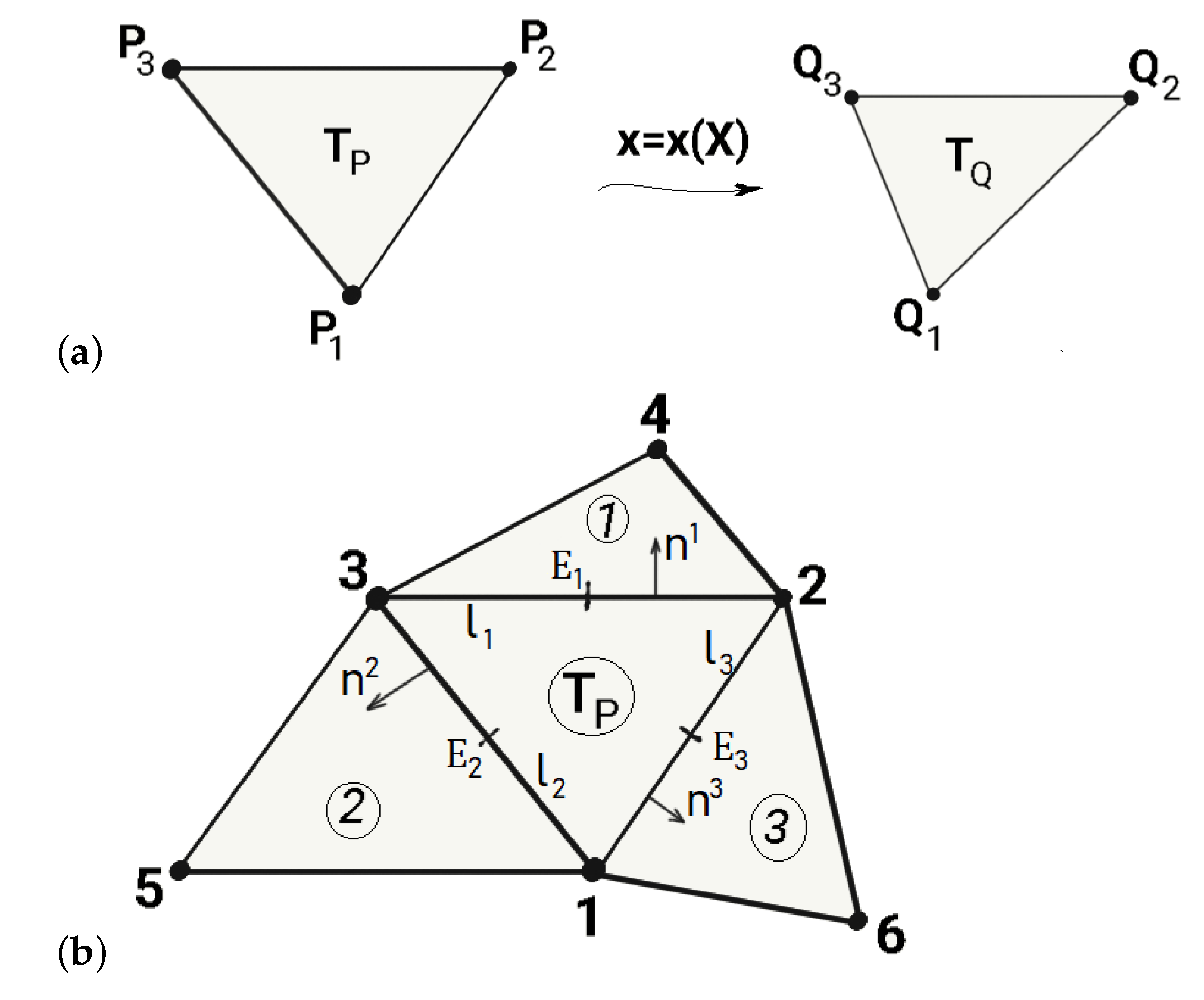
2.1. Shell Kinematics

We consider the deformation of a thin hyperelastic shell and employ the Kirchhoff–Love assumption that straight lines normal to the reference mid-surface remain normal to the mid-surface after deformation [16].
Let mapping Ψ : A Ω 0 R 3 define the mid-surface for an initial (before deformation) configuration. Here A R 2 is a compact set. A shell at the initial configuration S 0 is defined as
S 0 = { X R 3 | X ( ξ 1 , ξ 2 , ξ 3 ) = Ψ ( ξ 1 , ξ 2 ) + ξ 3 N ( ξ 1 , ξ 2 ) , where ( ξ 1 , ξ 2 ) A , ξ 3 [ H / 2 , H / 2 ] } ,
where H is an initial thickness of the shell and N is the unit normal to the mid-surface at the initial configuration.
Analogously, we can define an actual (deformed) configuration S t of the shell
S t = { x R 3 | x ( ξ 1 , ξ 2 , ξ 3 ) = ψ ( ξ 1 , ξ 2 ) + ξ 3 λ n ( ξ 1 , ξ 2 ) , where ( ξ 1 , ξ 2 ) A , ξ 3 [ H / 2 , H / 2 ] } ,
where ψ : A Ω t R 3 defines the mid-surface at the deformed configuration, λ = h / H relates the thickness at the undeformed and deformed configurations, h is the thickness of the deformed shell, and n is the unit normal to the mid-surface at the deformed configuration.
Convective coordinate systems for the initial (undeformed) and the current (deformed) configurations are:
G α = X ξ α = Ψ , α + ξ 3 N , α , α = 1 , 2 , G 3 = X ξ 3 = N ,
g α = x ξ α = ψ , α + ξ 3 ( λ n ) , α , α = 1 , 2 , g 3 = x ξ 3 = λ n ,
respectively. Hereafter, we denote the partial derivative f / ξ α by f , α .
The geometry of the mid-surface is given by the metric tensor with components
a α β = g α | ξ 3 = 0 · g β | ξ 3 = 0 = ψ , α · ψ , β , α , β = 1 , 2 ,
and the curvature tensor with components
κ α β = ψ , α β · n = 1 2 ψ , α · n , β + ψ , β · n , α , α , β = 1 , 2 .
The deformation gradient F for the shell is given by
F = x X = i = 1 3 g i G i ,
where a b a b T , G i = j = 1 3 ( G 1 ) i j G j , matrix G has entries G i j = G i · G j .
In the theory of thin shells, the right Cauchy-Green deformation tensor C = F T F = i , j = 1 3 g i · g j G i G j is reduced to the strain measure [15,16]
C = α , β = 1 2 c α β G α G β + λ 2 N N , c α β = a α β + 2 λ ξ 3 κ α β ,
which means
( C ) = C 11 C 12 0 C 12 C 22 0 0 0 C N .
Thus, tensor C is split into the surface (in-plane) part C S = α , β = 1 2 c α β G α G β and the out-of-plane part C N = λ 2 N N .

2.2. Constitutive Equations

The shell is assumed to be made of a hyperelastic material. This means there is an elastic potential (strain energy density function) W ( C ) such that the second Piola–Kirchhoff stress tensor S has the form [17]:
S = 2 W C = i , j = 1 3 s i j G i G j , s i j = 2 W c i j .
The elastic potential of an isotropic material is a function of three invariants [17]:
W ( C ) = W ˜ ( I 1 ( 3 D ) , I 2 ( 3 D ) , I 3 ( 3 D ) ) , I 1 ( 3 D ) = tr C , I 2 ( 3 D ) = ( tr C ) 2 tr C 2 / 2 , I 3 ( 3 D ) = det C = ( det F ) 2 .
For incompressible hyperelastic shells I 3 ( 3 D ) = 1 , and we rewrite the 3D invariants in terms of the surface invariants I 1 , J [18]:
I 1 ( 3 D ) = I 1 + J 2 , I 2 ( 3 D ) = J 2 + I 1 J 2 , where I 1 = tr C S , J 2 = det C S ,
therefore,
W ( C ) = W ^ ( I 1 , J ) .
According to (9), the constitutive equation of an incompressible isotropic hyperelastic material is written in the form of the plane stress state
S = α , β = 1 2 s α β G α G β , s α β = 2 W ^ c α β = 2 W ^ I 1 ( G 1 ) α β + J 2 W ^ J ( C S 1 ) α β ,
where ( A ) α β denotes α β -entry of matrix A .

2.3. Weak Formulation

We consider equilibrium of a thin shell subject to mixed boundary conditions and external forces with density b . Let the boundary of the mid-surface Ω t be split into two parts, Ω t = Γ u ( t ) Γ σ ( t ) , Γ u ( t ) = Γ ¯ u ( t ) . The mixed boundary conditions are
u = u ¯ o n   Γ u ( t ) , T n t = t ¯ o n   Γ σ ( t ) ,
where u = x X is the displacement of the mid-surface, n t is the unit outward normal to Ω t , T = ( 1 / det F ) F S F T is the Cauchy stress tensor, u ¯ and t ¯ are given displacement and tension on corresponding boundaries.
The equilibrium equations are based on the virtual work principle which states that the virtual work of the external forces δ W e x t is equal to the change in the total stored strain energy δ U [19]: Find u H ˜ 1 ( Ω t ) , H ˜ 1 ( Ω t ) : = v ( H 1 ( Ω t ) ) 3 , v = u ¯ on Γ u ( t ) , that
δ U δ W e x t = 0 ,
δ U = δ S 0 W ^ I 1 ( u , J ( u ) ) d V ,
δ W e x t = Γ σ ( t ) t ¯ · δ u d t + Ω t b · δ u d s .
Taking (8) and (13) into account, we can rewrite (15)–(17) as follows
δ U = Ω 0 l : δ a ( u ) d s + Ω 0 m : δ κ ( u ) d s ,
l = l 11 , l 22 , l 12 T , l i j = H / 2 H / 2 s i j d ξ 3 ,
m = m 11 , m 22 , m 12 T , m i j = H / 2 H / 2 s i j λ ξ 3 d ξ 3 ,
a = a 11 , a 22 , 2 a 12 T , κ = κ 11 , κ 22 , 2 κ 12 T .
The first term in (18) represents in-plane membrane behavior, whereas the second term characterizes the bending part (bending stiffness of the thin shell). The nodal hyperelastic force method [12] is applied to the discretization of the first term, and the bending part is discretized by the approach proposed by Oñate et al. [15].

2.4. Discretization

Given a consistent triangular mesh of the initial mid-surface configuration Ω 0 , we apply a combination of the P 1 finite elements for the membrane part and the rotation free bending elements for the shell bending part to the approximate solution of Equations (15), (17) and (18).
Let deformation of a triangle T P with vertices P 1 , P 2 , P 3 into a triangle T Q with vertices Q 1 , Q 2 , Q 3 be defined via mapping x ( X ) (see Figure 1a). Denote the area of the undeformed triangle T P by A P , the area of the deformed triangle T Q by A Q , and the unit normal to the plane of triangle T Q by n . The Jacobian of the deformation J = A Q / A P is one of the surface invariants.

2.4.1. Discretization of the Membrane Part

The hyperelastic nodal forces method is the P 1 finite element discretization of (15)–(17) in the membrane formulation [12].
The membrane part of the deformation of T P is discretized by
δ U m h = T P l : δ a ( u h ) d s ,
where u h is a P 1 finite element displacement and the corresponding nodal force for the i-th node of triangle T P is
F i m ( T P ) = δ U m h δ Q i = A P H δ W ^ h | ξ 3 = 0 δ Q i .
Here, the elastic potential W ^ h | ξ 3 = 0 is constant over the triangle T P since it is computed from the linear displacement u h . Formula (23) stems from the one-point quadrature for finding l i j in (19).

2.4.2. Bending Part

The bending part of the deformation of T P is discretized by
δ U b h = T P m : δ κ ( u h ) d s .
The contribution of the bending part to the total nodal force is obtained by rotation-free triangular shell elements [15]. The curvature tensor is recovered from nodal displacements of a patch Π P composed of the central element ( T P ) and three adjacent elements (in Figure 1b triangles 1, 2, 3). In notations of Figure 1b the local axis ξ 1 is directed along vector t 1 connecting nodes 1 and 2, the local axis ξ 3 is directed along the unit normal n to the plane of T P , the local axis ξ 2 is directed along n × t 1 .
The constant curvature field on each triangle T P is computed by
κ α β = 1 A P T P ψ , α β h · n d s ,
where A P is the area of the central element T P of the patch Π P in the undeformed configuration, ψ , α β h is the second partial derivative of P 2 vector function ψ h with given nodal values Q i in the patch Π P (Enhanced Basic Shell Triangle, EBST) [15].
The numerical integration in (25) gives the following expression for the curvature tensor components
κ α β = h α β · n , h α β = k = 1 3 1 2 L k , α M ψ , β h ( E k ) + L k , β M ψ , α h ( E k ) , α , β = 1 , 2 ,
where L k , 1 M , L k , 2 M T = l k 2 A P n 1 k , n 2 k T , n k = n 1 k , n 2 k T denotes the outer normal to the k-th edge of the central element T P in the initial configuration (see Figure 1b), l k and E k denote the length and the middle point of the k-th edge, respectively.
Equation (26) relates the curvature variation δ κ with vector δ Q = ( n · δ Q 1 , n · δ Q 2 , n · δ Q 3 , n · δ Q 4 , n · δ Q 5 , n · δ Q 6 ) T and the curvature matrix B b [15]
δ κ = B b δ Q .
Bending forces at the i-th node of the patch Π P are calculated by
F j b = A P δ U b h δ Q j , j = 1 , , 6 ,
which implies the patch Π P contribution to the nodal bending forces
( F 1 b , F 2 b , F 3 b , F 4 b , F 5 b , F 6 b ) = A P n ( B b T m ) .

2.4.3. Discretized Equilibrium Equations

The equilibrium Equations (15)–(21) form a local nonlinear system for new positions Q i of mesh nodes. Assembling local contributions of all triangles T P results in the static equilibrium for the i-th node
T P Σ i F i m ( T P ) + F i , e x t ( T P ) + p a t c h Π i F i b = 0 , F i , e x t ( T P ) = Γ σ ( t ) T Q t ¯ λ i d s + T Q b λ i d x ,
where Σ i is the set of triangles sharing the i-th node and Π i is the set of patches containing the i-th node.
Equation (30) form the system of algebraic equations
F ( Q ) = 0
which is solved by the damped Newton method Q k + 1 = Q k τ ( F ( Q k ) 1 F ( Q k ) . Parameter τ < 1 is chosen to avoid the divergence of iterations, in all experiments τ = 0.5 except the conservative loading of a cantilever where τ = 0.9 .

3. Numerical Results

We begin the study of our formulation with several benchmark problems for thin shells [20].

3.1. Benchmarks

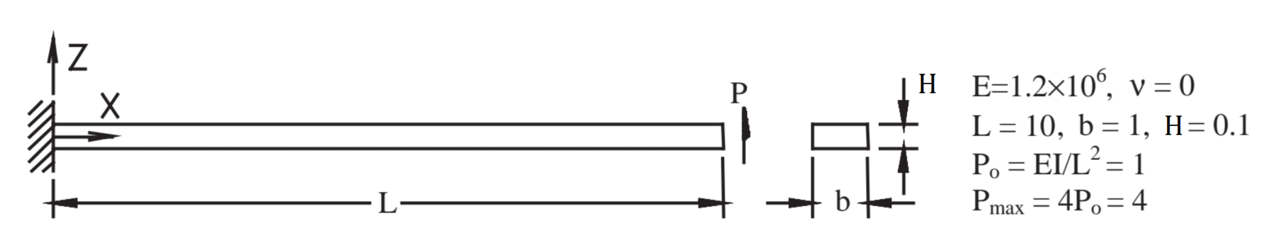
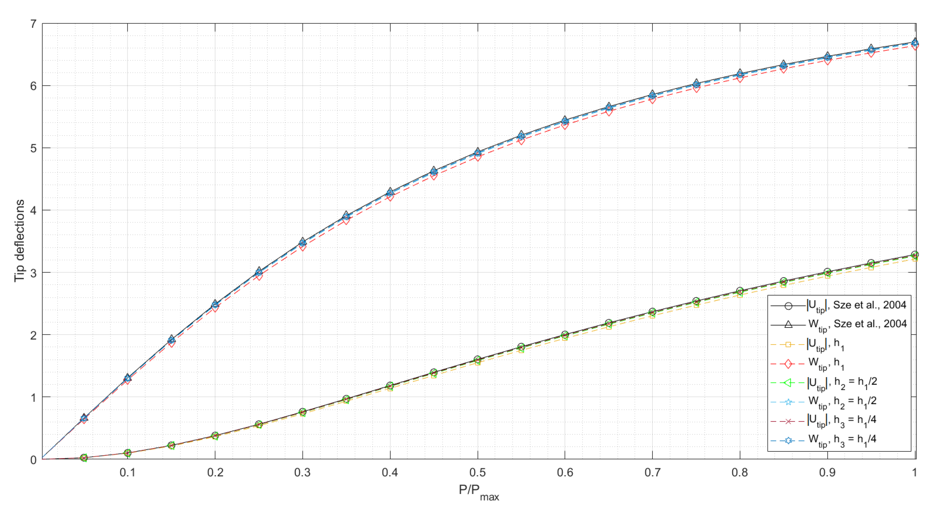
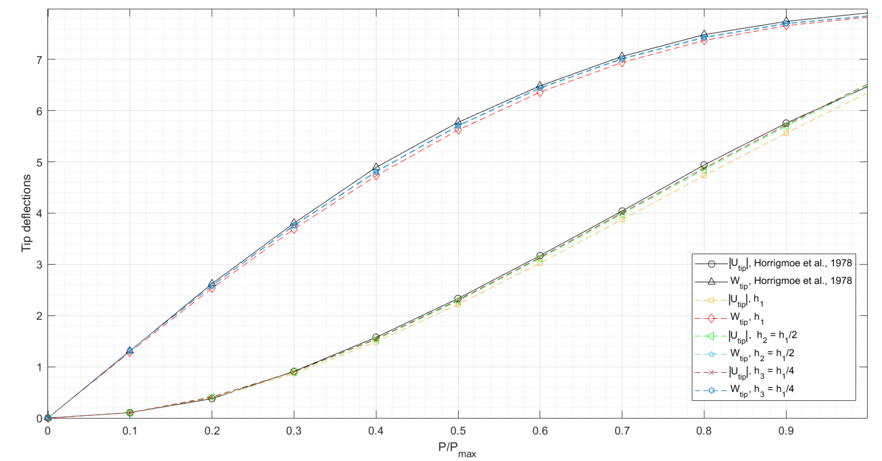
3.1.1. Cantilever Subjected to End Shear Force

We consider a cantilever made of the St-Venant–Kirchhoff (SVK) material subjected to the end shear force 0 P P max . Geometry setting and elastic constants (Young modulus E and Poisson’s coefficient ν ) are presented in Figure 2.
For this benchmark ν = 0 , and we cannot use (11) to express the elastic potential in terms of the surface invariants ( I 1 , J ) , since (11) was derived under the incompressibility condition ν = 1 / 2 . For arbitrary ν , the plane stress state s 13 = s 23 = s 33 = 0 implies the following elastic potential for SVK material in terms of ( I 1 , J ) :
W ^ S V K ( I 1 , J ) = μ λ 4 ( λ + 2 μ ) ( I 1 2 ) 2 + μ 4 ( I 1 1 ) 2 2 J 2 + 1 , λ = E ν ( 1 ν 2 ) , μ = E 2 ( 1 + ν ) .
The clamped boundary condition is implemented following [15]. If a triangle T P is adjacent to a free edge of Ω 0 , its patch Π P is incomplete and we estimate the curvature tensor from the extra condition of vanishing linearized moments
n f T M ( 0 ) n f = 0 , n f T M ( 0 ) t f = 0 .
Here, n f = ( n 1 , n 2 ) T and t f = ( n 2 , n 1 ) T denote normal and tangent vectors to the free edge in the initial configuration Ω 0 , M ( 0 ) denotes a 2 × 2 matrix with components
M i j ( 0 ) = λ 2 H 3 6 α , β = 1 2 s i j c α β κ α β .
The Equation (33) stems from (20), (8) and linearization of the second Piola–Kirchoff stress tensor S .
We consider conservative and non-conservative loadings of the cantilever [21]. The first one is a standard load P with the fixed direction normal to the initial mid-surface Ω 0 . The second one is a load P perpendicular to the current mid-surface Ω t .
The equilibrium is searched on three quasi-uniform unstructured triangular meshes with mesh sizes h 1 = 0.1 , h 2 = h 1 / 2 , h 3 = h 1 / 4 . The load-deflection curves for the conservative and non-conservative loadings are shown in Figure 3 and Figure 4, respectively. The curves converge to the reference curves [20,21] as the mesh is refined, with a relative pointwise error of less than 2%.

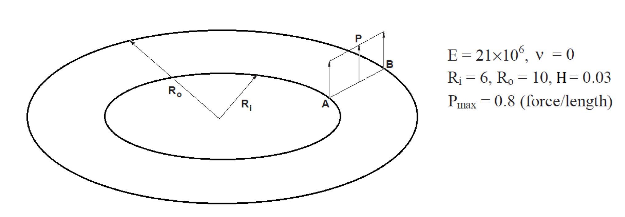
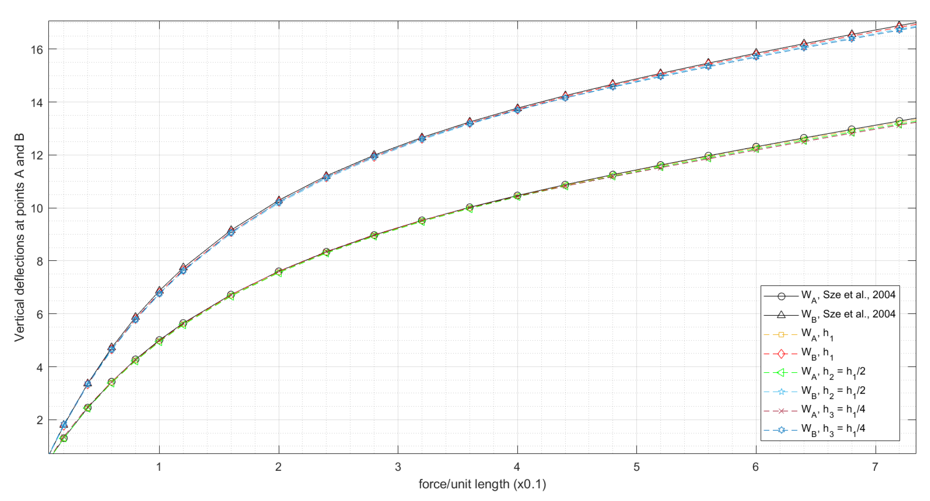
3.1.2. Slit Annular Plate Subjected to Lifting Line Force

The next benchmark addresses a slit annular plate made of SVK material [20]. The line force P is applied at one end of the slit, while the other end of the slit is fully clamped, see Figure 5. The free edge and clamped boundary conditions were imposed similarly to the cantilever benchmark.
The equilibrium is searched on three quasi-uniform unstructured triangular meshes with mesh sizes h 1 = 0.2 , h 2 = h 1 / 2 , h 3 = h 1 / 4 . The load–deflection curves are shown in Figure 6. The relative pointwise error with respect to the reference curve [20] is less than 2% as well.

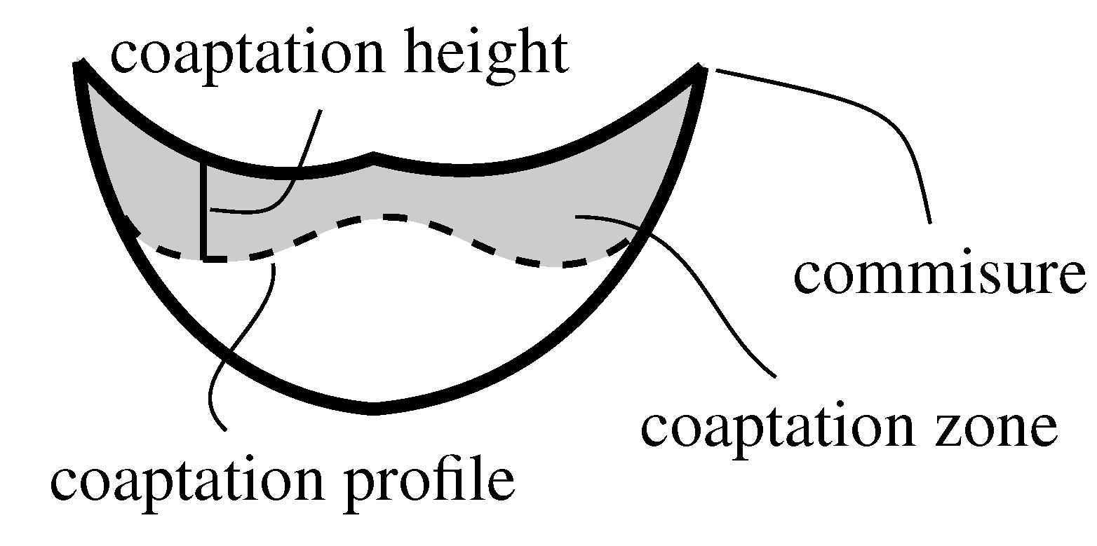
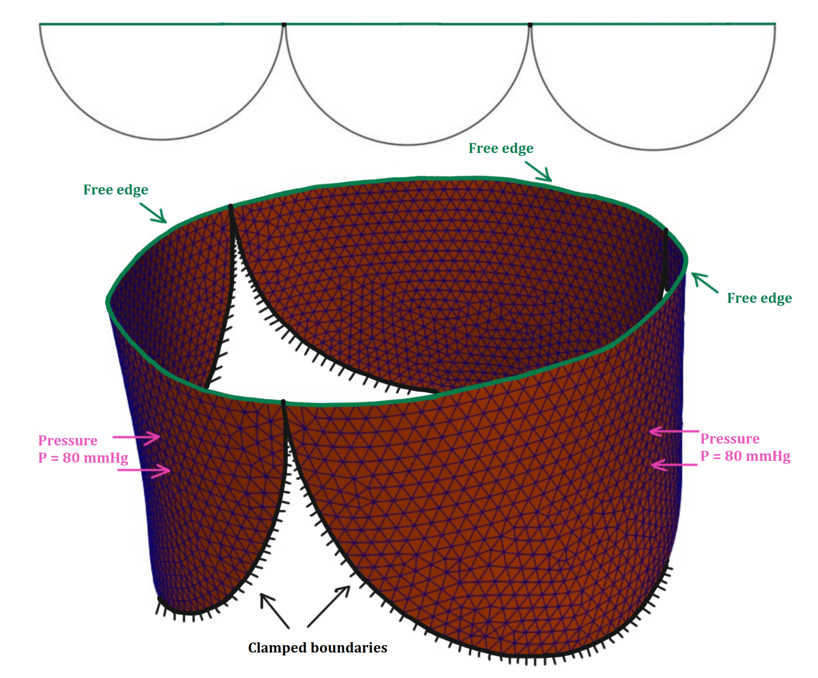
3.2. Aortic Valve in Diastolic State

The competence of a reconstructed aortic valve is given by cusps coaptation characteristics. The cusps (leaflets) can not interpenetrate, they interact with each other forming coaptation zones. The coaptation zone and other coaptation characteristics for a cusp are schematically represented in Figure 7.
To estimate how bending stiffness affects a reconstructed tricuspid aortic valve competence, we consider idealized geometries of three leaflets and the aortic root [10]. Each leaflet is represented by a semicircle with 20 mm diameter. The leaflet is fixed along its semi-circumference to the inside wall of a cylinder (aortic root) with 60 mm circumference. The idealized aortic valve model combines three identical semicircular leaflets, arranged circumferentially around the inside wall of the cylinder. Such a valve model defines the initial configuration. Each leaflet is subjected to diastolic blood pressure of 80 mm Hg. The boundary conditions are presented in Figure 8. The numerical solution is computed on two quasi-uniform unstructured triangular meshes with mesh sizes h 1 = 0.5 mm (coarse), h 2 = h 1 / 2 (fine).
We compare the coaptation characteristics of the idealized aortic valve obtained by the membrane and the thin shell models. The cusps are assumed to be cut from treated human pericardium. The mechanical properties of fresh and treated human pericardium are not clear: according to [22], fresh and treated human pericardium is isotropic whereas animal pericardium is anisotropic; according to [23], fresh and treated human pericardium is anisotropic. Glutaraldehyde-treated autopericardium is known to be significantly stiffer than native autopericardium. In the present work, we compare only isotropic incompressible materials (St.Venant–Kirchhoff, neo-Hookean, Gent), and vary their elastic moduli. For the last two materials, the elastic potentials are
W ^ n e o H o o k e a n = μ / 2 ( I 1 + J 2 3 ) ,
W ^ G e n t = J m μ / 2 ln ( 1 ( I 1 + J 2 3 ) / J m ) ,
where μ = E / 3 is the shear modulus, J m is a material constant. Models (31), (34), (35) benefit from the physical meanings of their parameters.
Each valve cusp is represented by an oriented triangulated surface, whose position in the 3D space provides the static equilibrium of the three closed cusps under blood diastolic pressure. The equilibrium implies the following for each free mesh node with index i
F i p + F i s + F i c = 0 ,
where F i p , F i s , F i c are the force of diastolic blood pressure, the elastic force and the contact force due to reaction of the other leaflets [11], respectively.
To find the static equilibrium, we apply Algorithm 1 to our inhouse code. Contact detection and contact forces are computed in lines 11–31 of the Algorithm, following the idea of real-time simulation [24] and Soft–Soft contact processing algorithm [25].
Algorithm 1 Solution of the static equilibrium equation and computation of the contact forces
 Require:
initial positions of leaflets meshes nodes x 0  
1:
set relaxation coefficient λ , contact distance parameter d c  
2:
set maximal allowed number of relaxation iterations m a x i t s , convergence parameter ε a b s  
3:
set i = 0  
4:
repeat 
5:
    compute elastic forces F e F e ( x i )  
6:
    compute pressure forces F p F p ( x i )  
7:
    compute contact forces F c ContactForces( x i , F e + F p , λ , d c )  
8:
     x i + 1 = x i + λ ( F e + F p + F c )  
9:
     i i + 1  
10:
until | | F c + F e + F p | | ε a b s or i m a x i t s  
      
Contact detection and contact forces
11:
procedureContactForces( x , F , λ , d c
12:
    for mesh node N: nodal position x ( N ) , nodal forces F ( N )                                               ▹ initialization  
13:
    for triangle T with nodes N 1 , N 2 , N 3 : matrix of nodal positions x ( T ) = ( x ( N 1 ) , x ( N 2 ) , x ( N 3 ) ) , matrix of nodal forces F ( T ) = ( F ( N 1 ) , F ( N 2 ) , F ( N 3 ) )  
14:
    define p r o j ( N , T ) as the nearest point of the triangle T to the node N
15:
    define d i s t ( N , T ) = | | p r o j ( N , T ) x ( N ) | | 2  
16:
    set contact forces to zero: F c = 0  
17:
    find a set of pairs L = { ( N , T ) | N   and   T are   in   meshes   of   different   leaflets ,   d i s t ( N , T ) < d c + 2 λ | | F ( N ) | | 2 }  
18:
    for all  ( N , T ) L  do  
19:
         F n F ( N ) + F c ( N ) , F T F ( T ) + F c ( T )  
20:
         P p r o j ( N , T ) , d d i s t ( N , T )  
21:
        compute barycentric coordinates w = ( w 1 , w 2 , w 3 ) T of P on triangle T  
22:
         n = ( x ( N ) P ) / d  
23:
         m d c + 2 λ | | F n | | 2 , m 1 d + 2 λ F n · n  
24:
         v λ ( F n + F T · w )  
25:
        if  m > d and v · n > 0  then 
26:
            j 1 2 ( m m 1 v · n ) n  
27:
           modify F c at node N: F c ( N ) F c ( N ) + 1 λ j  
28:
           modify F c at triangle T nodes: F c ( T ) F c ( T ) 1 λ j w T  
29:
        end if 
30:
    end for 
31:
    return  F c  
32:
end procedure
Computed coaptation characteristics from Table 1 demonstrate that bending stiffness reduces significantly the coaptation zone. Comparison of the coaptation characteristics computed on the coarse and the fine grids indicates that the mesh convergence is achieved. Stiff cusps ( E = 10 MPa) do not coapt when bending stiffness is incorporated. Though they do not coapt properly even in the membrane formulation due to improper leaflet design. Less stiff cusps provide the coaptation. The coaptation height depends on elastic modulus E but does not depend on the material model which confirms the same observation in [11].
In Table 2 we present the CPU time for different models and materials on the coarse mesh. The simulations were run on a laptop Intel Core with i5-8250U CPU 1.60 GHz. For the analysis of the computational work we refer to the next section.
Figure 9a,b demonstrates the closed aortic valve for the neo-Hookean material with E = 1 MPa; the other materials give similar shapes. Convexity at the boundary and the incomplete coaptation for the shell-based model near the commissure points (Figure 9c) are caused by the clamped boundary condition. One can also observe the incomplete coaptation at the center of the leaflets for the shell-based model, due to te insufficient length of the cusps. The membrane-based model for the materials with E = 1 MPa provides the complete coaptation; the gap between the cusps is due to visualization of the mid-surfaces, which are distanced from each other at 0.5 mm, the cusps thickness.

4. Discussion

Coaptation characteristics are crucial in assessment of competence of reconstructed aortic valves. The valve cusps coaptation can be evaluated via shell [26] or membrane [10] formulations. In this paper, we compare both formulations in terms of coaptation characteristics for the first time. In particular, we study the impact of bending stiffness on the aortic valve closure. Our numerical thin shell model is based on a combination of the hyperelastic nodal forces method and the rotation free finite elements.
The numerical shell model is verified on several popular benchmarks for thin shell analysis. The relative error with respect to the reference solutions does not exceed 1–2%.
We apply our numerical shell and membrane formulations to model the closure of the idealized aortic valve varying hyperelastic models and their shear moduli. The coaptation characteristics become sensitive to the bending stiffness and almost insensitive to the elastic potential.
Our study has several limitations. First, the idealized leaflet design [10] leads to incomplete coaptation for both membrane and shell models of stiff cusps. Advanced leaflet designs [3,4], result in better coaptation characteristics. Second, our isotropic constitutive models may overestimate the impact of bending stiffness. Third, the clamped boundary condition may require modifications in order to avoid regurgitation in the vicinity of the commissures. Fourth, the CPU time of computing coaptation for the shell formulation is prohibitively large for patient-specific leaflet shape optimization and our numerical method for shells has to be more efficient in terms of CPU time.
In our future work, we shall address different known leaflet designs, anisotropic materials, more realistic boundary conditions accounting leaflet suturing and employ patient-specific geometry of the aortic root based on segmentation algorithms [27].

Author Contributions

Conceptualization, V.S. and Y.V.; methodology, V.S. and A.L.; software, A.L.; investigation, V.S., A.L. and Y.V.; draft preparation, V.S. and Y.V.; supervision, Y.V. All authors have read and agreed to the published version of the manuscript.

Funding

The study was performed at Marchuk Institute of Numerical Mathematics RAS and supported by the Russian Science Foundation (project 21-71-30023).

Institutional Review Board Statement

Not applicable.

Informed Consent Statement

Not applicable.

Data Availability Statement

Not applicable.

Conflicts of Interest

The authors declare no conflict of interest.

References

  1. Coffey, S.; Cairns, B.J.; Iung, B. The modern epidemiology of heart valve disease. Heart 2016, 102, 75–85. [Google Scholar] [CrossRef]
  2. Rankin, J.S.; Nöbauer, C.; Crooke, P.S.; Schreiber, C.; Lange, R.; Mazzitelli, D. Techniques of autologous pericardial leaflet replacement for aortic valve reconstruction. Ann. Thorac. Surg. 2014, 98, 743–745. [Google Scholar] [CrossRef]
  3. Labrosse, M.R.; Beller, C.J.; Robicsek, F.; Thubrikar, M.J. Geometric modeling of functional trileaflet aortic valves: Development and clinical applications. J. Biomech. 2006, 39, 2665–2672. [Google Scholar] [CrossRef] [PubMed]
  4. Ozaki, S.; Kawase, I.; Yamashita, H.; Uchida, S.; Nozawa, Y.; Takatoh, M.; Hagiwara, S. A total of 404 cases of aortic valve reconstruction with glutaraldehyde-treated autologous pericardium. J. Thorac. Cardiovasc. Surg. 2014, 147, 301–306. [Google Scholar] [CrossRef] [PubMed] [Green Version]
  5. Zakerzadeh, R.; Hsu, M.C.; Sacks, M.S. Computational methods for the aortic heart valve and its replacements. Expert Rev. Med. Devices 2017, 14, 849–866. [Google Scholar] [CrossRef] [PubMed]
  6. Sturla, F.; Votta, E.; Stevanella, M.; Conti, C.A.; Redaelli, A. Impact of modeling fluid–structure interaction in the computational analysis of aortic root biomechanics. Med. Eng. Phys. 2013, 35, 1721–1730. [Google Scholar] [CrossRef]
  7. Berra, I.G.; Hammer, P.E.; Berra, S.; Irusta, A.O.; Ryu, S.C.; Perrin, D.P.; Vasilyev, N.V.; Cornelis, C.J.; Delucis, P.G.; Pedro, J. An intraoperative test device for aortic valve repair. J. Thorac. Cardiovasc. Surg. 2019, 157, 126–132. [Google Scholar] [CrossRef]
  8. Pappalardo, O.A.; Sturla, F.; Onorati, F.; Puppini, G.; Selmi, M.; Luciani, G.B.; Faggian, G.; Redaelli, A.; Votta, E. Mass-spring models for the simulation of mitral valve function: Looking for a trade-off between reliability and time-efficiency. Med. Eng. Phys. 2017, 47, 93–104. [Google Scholar] [CrossRef]
  9. Hammer, P.E.; Pedro, J.; Howe, R.D. Anisotropic mass-spring method accurately simulates mitral valve closure from image-based models. In Functional Imaging and Modeling of the Heart. FIMH 2011. Lecture Notes in Computer Science; Metaxas, D.N., Axel, L., Eds.; Springer: Berlin/Heidelberg, Germany, 2011; Volume 6666, pp. 233–240. [Google Scholar]
  10. Hammer, P.E.; Sacks, M.S.; Pedro, J.; Howe, R.D. Mass-spring model for simulation of heart valve tissue mechanical behavior. Ann. Biomed. Eng. 2011, 39, 1668–1679. [Google Scholar] [CrossRef] [Green Version]
  11. Salamatova, V.Y.; Liogky, A.A.; Karavaikin, P.A.; Danilov, A.A.; Kopylov, P.Y.; Kopytov, G.V.; Kosukhin, O.N.; Pryamonosov, R.A.; Shipilov, A.A.; Yurova, A.S.; et al. Numerical assessment of coaptation for auto-pericardium based aortic valve cusps. Russ. J. Numer. Anal. Math. Model. 2019, 34, 277–287. [Google Scholar] [CrossRef]
  12. Salamatova, V.Y.; Liogky, A.A. Method of Hyperelastic Nodal Forces for Deformation of Nonlinear Membranes. Differ. Equ. 2020, 56, 950–958. [Google Scholar] [CrossRef]
  13. Murdock, K.; Martin, C.; Sun, W. Characterization of mechanical properties of pericardium tissue using planar biaxial tension and flexural deformation. J. Mech. Behav. Biomed. Mater. 2018, 77, 148–156. [Google Scholar] [CrossRef] [PubMed]
  14. Gärdsback, M.; Tibert, G. A comparison of rotation-free triangular shell elements for unstructured meshes. Comput. Methods Appl. Mech. Eng. 2007, 196, 5001–5015. [Google Scholar] [CrossRef]
  15. Oñate, E.; Flores, F.G. Advances in the formulation of the rotation-free basic shell triangle. Comput. Methods Appl. Mech. Eng. 2005, 194, 2406–2443. [Google Scholar] [CrossRef]
  16. Tepole, A.B.; Kabaria, H.; Bletzinger, K.U.; Kuhl, E. Isogeometric Kirchhoff–Love shell formulations for biological membranes. Comput. Methods Appl. Mech. Eng. 2015, 293, 328–347. [Google Scholar] [CrossRef] [Green Version]
  17. Holzapfel, G. Nonlinear Solid Mechanics: A Continuum Approach for Engineering Science; John Wiley & Sons Ltd.: Chichester, UK, 2000; p. 470. [Google Scholar]
  18. Lu, J.; Zhou, X.; Raghavan, M.L. Inverse method of stress analysis for cerebral aneurysms. Biomech. Model. Mechanobiol. 2008, 7, 477–486. [Google Scholar] [CrossRef]
  19. Ciarlet, P.G. Mathematical Elasticity. Volume I: Three-Dimensional Elasticity; North-Holland: Amsterdam, The Netherlands, 1988; p. 451. [Google Scholar]
  20. Sze, K.Y.; Liu, X.H.; Lo, S.H. Popular benchmark problems for geometric nonlinear analysis of shells. Finite Elem. Anal. Des. 2004, 40, 1551–1569. [Google Scholar] [CrossRef]
  21. Horrigmoe, G.; Bergan, P.G. Nonlinear analysis of free-form shells by flat finite elements. Comput. Methods Appl. Mech. Eng. 1978, 16, 11–35. [Google Scholar] [CrossRef]
  22. Aguiari, P.; Fiorese, M.; Iop, L.; Gerosa, G.; Bagno, A. Mechanical testing of pericardium for manufacturing prosthetic heart valves. Interact. Cardiovasc. Thorac. Surg. 2015, 22, 72–84. [Google Scholar] [CrossRef] [Green Version]
  23. Zigras, T.C. Biomechanics of Human Pericardium: A Comparative Study of Fresh and Fixed Tissue. Ph.D. Thesis, McGill University, Montreal, QC, Canada, 2007. [Google Scholar]
  24. Raghupathi, L.; Grisoni, L.; Faure, F.; Marchal, D.; Cani, M.P.; Chaillou, C. An intestinal surgery simulator: Real-time collision processing and visualization. IEEE Trans. Vis. Comput. Graph. 2004, 10, 708–718. [Google Scholar] [CrossRef] [PubMed]
  25. Method btSoftBody::PSolve_SContacts. Available online: https://github.com/bulletphysics/bullet3/blob/master/src/BulletSoftBody/btSoftBody.cpp (accessed on 20 June 2021).
  26. Marom, G.; Haj-Ali, R.; Raanani, E.; Schäfers, H.J.; Rosenfeld, M. A fluid-structure interaction model of the aortic valve with coaptation and compliant aortic root. Med. Biol. Eng. Comput. 2012, 50, 173–182. [Google Scholar] [CrossRef] [PubMed]
  27. Danilov, A.; Ivanov, Y.; Pryamonosov, R.; Vassilevski, Y. Methods of graph network reconstruction in personalized medicine. Int. J. Numer. Methods Biomed. Eng. 2016, 32, e02754. [Google Scholar] [CrossRef] [PubMed]
Figure 1. (a) Triangle before and after deformation. (b) Patch of elements including the central triangle T P and three adjacent elements (1, 2, and 3).
Mathematics 09 01450 g001
Figure 2. Cantilever subjected to end shear force.
Mathematics 09 01450 g002
Figure 3. Load–deflection curves for the cantilever subjected to end shear force (conservative loading). U t i p and W t i p are the vertical and horizontal tip deflections. The values of U t i p are negative.
Mathematics 09 01450 g003
Figure 4. Load–deflection curves for the cantilever subjected to end shear force (non-conservative loading). U t i p and W t i p are the vertical and horizontal tip deflections. The values of U t i p are negative.
Mathematics 09 01450 g004
Figure 5. The slit annular plate loaded with the line force P.
Mathematics 09 01450 g005
Figure 6. Load–deflection curves for the slit annular plate lifted by line force P. W A and W B are the vertical tip deflections of points A and B, respectively.
Mathematics 09 01450 g006
Figure 7. Coaptation characteristics for a cusp.
Mathematics 09 01450 g007
Figure 8. Schematic representation of the idealized aortic valve in the initial configuration, the boundary conditions and the computational mesh (mesh size h 1 ).
Mathematics 09 01450 g008
Figure 9. Mid-surface positions of the neo-Hookean ( E = 1 MPa) cusps with 0.5 mm thickness: (a) shell-based coaptation, (b) membrane-based coaptation, (c) trace of two leaflets on the cut plane distanced from the aortic center by 5 mm; shell-based curve (red) and membrane-based curve (blue).
Mathematics 09 01450 g009
Table 1. Comparison of maximal coaptation heights and free edge lengths computed by different models for two meshes with mesh sizes h 1 and h 2 , respectively. Symbol * denotes the lack of coaptation.
Model Max. CoaptationFree Edge
Height, mmLength, mm
h 1 h 2 h 1 h 2
SVK E = 1 MPa, ν = 0.5 (membrane) 3.51 3.45 23.20 23.15
E = 1 MPa, ν = 0.5 (shell) 0.4 0.37 23.31 23.35
Neo-Hookean E = 1 MPa, μ = E / 3 (membrane) 3.72 3.72 23.96 23.91
E = 1 MPa, μ = E / 3 (shell) 0.73 0.76 23.75 23.77
Gent E = 1 MPa, μ = E / 3 , J m = 2.3 (membrane) 3.71 3.70 23.76 23.71
E = 1 MPa, μ = E / 3 , J m = 2.3 (shell) 0.58 0.6 23.61 23.61
SVK E = 10 MPa, ν = 0.5 (membrane) 0.71 0.81 20.82 20.93
E = 10 MPa, ν = 0.5 (shell)** 20.94 20.99
Neo-Hookean E = 10 MPa, μ = E / 3 (membrane) 0.67 0.66 20.93 20.99
E = 10 MPa, μ = E / 3 (shell)** 20.99 21.03
Gent E = 10 MPa, μ = E / 3 , J m = 2.3 (membrane) 0.66 0.67 20.91 20.90
E = 10 MPa, μ = E / 3 , J m = 2.3 (shell)** 20.98 21.02
Table 2. CPU times for different models on the coarse mesh.
Model CPU Time, s
SVK E = 1 MPa, ν = 0.5 (membrane)220
E = 1 MPa, ν = 0.5 (shell)3761
Neo-Hookean E = 1 MPa, μ = E / 3 (membrane)157
E = 1 MPa, μ = E / 3 (shell)3940
Gent E = 1 MPa, μ = E / 3 , J m = 2.3 (membrane)170
E = 1 MPa, μ = E / 3 , J m = 2.3 (shell)5047
SVK E = 10 MPa, ν = 0.5 (membrane)831
E = 10 MPa, ν = 0.5 (shell)5736
Neo-Hookean E = 10 MPa, μ = E / 3 (membrane)810
E = 10 MPa, μ = E / 3 (shell)5561
Gent E = 10 MPa, μ = E / 3 , J m = 2.3 (membrane)832
E = 10 MPa, μ = E / 3 , J m = 2.3 (shell)4496
Publisher’s Note: MDPI stays neutral with regard to jurisdictional claims in published maps and institutional affiliations.

