Article

Quasistatic Porous-Thermoelastic Problems: An a Priori Error Analysis

by
Jacobo Baldonedo
1,
José R. Fernández
2,* and
José A. López-Campos
1
1
CINCTEX, Departamento de Ingeniería Mecánica, Universidade de Vigo, Máquinas y Motores Térmicos y Fluídos, 36310 Vigo, Spain
2
Departamento de Matemática Aplicada I, Universidade de Vigo, 36310 Vigo, Spain
*
Author to whom correspondence should be addressed.
Mathematics 2021, 9(12), 1436; https://doi.org/10.3390/math9121436
Submission received: 12 May 2021 / Revised: 16 June 2021 / Accepted: 17 June 2021 / Published: 20 June 2021
(This article belongs to the Special Issue Applied Mathematics and Solid Mechanics)

Abstract

:
In this paper, we deal with the numerical approximation of some porous-thermoelastic problems. Since the inertial effects are assumed to be negligible, the resulting motion equations are quasistatic. Then, by using the finite element method and the implicit Euler scheme, a fully discrete approximation is introduced. We prove a discrete stability property and a main error estimates result, from which we conclude the linear convergence under appropriate regularity conditions on the continuous solution. Finally, several numerical simulations are shown to demonstrate the accuracy of the approximation, the behavior of the solution and the decay of the discrete energy.

1. Introduction

Since the first work by Cosserat and Cosserat [1], who introduced the theory of the so-called micropolar materials, there were several models to extend it to other type of elastic materials. For instance, assuming that the bulk density is equal to the product of the density matrix by the volume fraction, Cowin and Nunziato [2,3] introduced the theory of elastic solids with voids, where the pores are distributed within the material. Rocks, woods, biological materials (as bones), or soils are some examples of this kind of materials. Later, heat effects were also included and the number of papers dealing with these porous-thermoelastic problems is really huge (see, among others, [4,5,6,7,8,9]), and their numerical issues [10,11,12,13,14,15].
It is well-known that there is a paradox of instantaneous propagation of the thermal waves in the classical heat theory provided by the Fourier law. In order to overcome it, several proposals were made since 1990. One of them was proposed by Green and Naghdi [16], where a new variable, the thermal displacement, was considered. Here, we will study the type II theory, which is also called thermoelasticity without energy dissipation.
In this paper, we also assume that the process is quasi-static and so, we neglect the inertia term in the motion equation. This expression was intorduced by Mosconi [17] and we note that the system of equations that we obtain differs substantially from the original one, leading to a mixture of some parabolic and hyperbolic equations. One interesting question is, therefore, if the behavior of the solution with respect to the time variable remains unaltered in the quasi-static case. The number of contributions has increased over the last years (see, among others, [18,19,20,21]). In a recent article by Magaña and Quintanilla [22], they considered that this quasi-static hypothesis was also imposed in the volume fraction and in the temperature. So, it led to a set of different problems for which they proved the existence and uniqueness of solution and the slow or exponential energy decay. Here, we continue this research, aiming to provide an a priori error analysis of a fully discrete approximation and to perform some numerical simulations.
The paper is structured in the following way. In Section 2, we describe the thermo-mechanical problem following [22] and we recall an existence and uniqueness result. Then, in Section 3, we present the discrete problem, using the finite element method to approximate the spatial variable and the implicit Euler scheme to discretize the time derivatives. A discrete stability property and a priori error estimates are proved, from which the linear convergence of the algorithm is deduced under adequate additional regularity. Finally, in Section 4, some numerical results are presented to demonstrate the accuracy of the algorithm and the behavior of the solution.

2. The Thermo-Mechanical Problem and Its Variational Formulation

In this section, we describe briefly the problem and we recall an existence and uniqueness result (see [22] for further details).
Without loss of generality, we suppose that the spatial variable x lies in the interval [ 0 , ] and that the time t goes from 0 to T, where T > 0 denotes the final time. Moreover, the subscript x indicates the spatial derivative and a dot over a variable represents the time derivative.
Defining the displacement field, the porosity field and the temperature field by u, φ and θ , respectively, the porous-thermo-mechanical problem is written as follows.
Find the displacement field u : [ 0 , ] × [ 0 , T ] R , the porosity field φ : [ 0 , ] × [ 0 , T ] R and the temperature field θ : [ 0 , ] × [ 0 , T ] R such that
μ * u ˙ x x μ u x x = b φ x β θ x in ( 0 , ) × ( 0 , T ) ,
J φ ¨ = δ φ x x b u x ξ φ + m θ in ( 0 , ) × ( 0 , T ) ,
c θ ˙ = β u ˙ x m φ ˙ + κ * θ x x in ( 0 , ) × ( 0 , T ) ,
u ( 0 , t ) = u ( , t ) = φ ( 0 , t ) = φ ( , t ) = θ ( 0 , t ) = θ ( , t ) for a . e . t ( 0 , T ) ,
u ( x , 0 ) = u 0 ( x ) , u ˙ ( x , 0 ) = v 0 ( x ) , φ ( x , 0 ) = φ 0 ( x ) for a . e . x ( 0 , ) ,
φ ˙ ( x , 0 ) = ψ 0 ( x ) , θ ( x , 0 ) = θ 0 ( x ) for a . e . x ( 0 , ) ,
where μ * , μ , b, β , J, δ , ξ , m, c and κ * are constitutive parameters satisfying some conditions which will be detailed later, and u 0 , v 0 , φ 0 , ψ 0 and θ 0 are given initial conditions. The influence of the dissipation constants μ * and κ * will be numerically studied in Section 4.2.
In what follows, we obtain the variational formulation of the thermo-mechanical problem (1)–(6). Let Y = L 2 ( 0 , ) , and denote by ( · , · ) the scalar product in this space, with corresponding norm · Y . Moreover, let us define V = H 0 1 ( 0 , ) with norm · V .
Let us denote by v = u ˙ and ψ = φ ˙ the velocity and porosity speed. Therefore, integrating by parts it leads to the following variational formulation of problem (1)–(6).
Find the velocity field v : [ 0 , T ] V , the porosity speed ψ : [ 0 , T ] V and the temperature θ : [ 0 , T ] V such that v ( 0 ) = v 0 , ψ ( 0 ) = ψ 0 , θ ( 0 ) = θ 0 and, for a.e. t ( 0 , T ) and w , r , s V ,
μ * ( v x ( t ) , w x ) + μ ( u x ( t ) , w x ) = b ( φ x ( t ) , w ) + β ( θ ( t ) , w x ) ,
J ( ψ ˙ ( t ) , r ) + δ ( φ x ( t ) , r x ) + ξ ( φ ( t ) , r ) = m ( θ ( t ) , r ) b ( u x ( t ) , r ) ,
c ( θ ˙ ( t ) , s ) + κ * ( θ x ( t ) , s x ) = β ( v x ( t ) , s ) m ( ψ ( t ) , s ) ,
where the displacement and the porosity fields u and φ are recovered from the equations:
u ( t ) = 0 t v ( s ) d s + u 0 , φ ( t ) = 0 t ψ ( s ) d s + φ 0 .
The following existence and uniqueness result has been recently proved in [22].
Theorem 1.
Assume that the constitutive coefficients satisfy the following conditions:
μ > 0 , μ * > 0 , J > 0 , δ > 0 , ξ > 0 , c > 0 , κ * > 0 .
Then, there exists a unique solution
u C 1 ( [ 0 , T ] ; Y ) C ( [ 0 , T ] ; V ) , φ , θ C 1 ( [ 0 , T ] ; Y ) C ( [ 0 , T ] ; H 2 ( 0 , ) )
to problem (1)–(6).
Regarding the energy decay, it was also proved in [22] that the energy of the system related to problem (1)–(6) decays in a slow way. However, if we replace the Fourier law by the type II thermal law (see Remark 1), then using the theory of linear semigroups it was shown in [22] that the energy decays in an exponential way.

3. An a Priori Error Analysis

In this section, we study a fully discrete approximation of the porous-thermo-mechanical problem (1)–(6) described in the previous section. First, in order to obtain the spatial approximation, we assume that the interval [ 0 , ] is divided into M subintervals a 0 = 0 < a 1 < < a M = of length h = a i + 1 a i = / M . Therefore, to approximate the variational space V, we define the finite dimensional space V h V given by
V h = { w h C ( [ 0 , ] ) ; w | [ a i , a i + 1 ] h P 1 ( [ a i , a i + 1 ] ) i = 0 , , M 1 , w h ( 0 ) = w h ( ) = 0 } ,
where P 1 ( [ a i , a i + 1 ] ) represents the space of polynomials of degree less or equal to one in the subinterval [ a i , a i + 1 ] ; i.e., the finite element space V h is made of continuous and piecewise affine functions. Here, h > 0 denotes the spatial discretization parameter. Furthermore, let the discrete initial conditions u 0 h , v 0 h , φ 0 h , ψ 0 h and θ 0 h be defined as
u 0 h = P h u 0 , v 0 h = P h v 0 , φ 0 h = P h φ 0 , ψ 0 h = P h ψ 0 , θ 0 h = P h θ 0 ,
where P h is the classical finite element interpolation operator over V h (see [23]).
Secondly, we consider a uniform partition of the time interval [ 0 , T ] , denoted by 0 = t 0 < t 1 < < t N = T , with step size k = T / N and nodes t n = n k for n = 0 , 1 , , N .
Therefore, using the well-known implicit Euler scheme, the fully discrete approximations of the above variational problem are the following.
Find the discrete velocity v h k = { v n h k } n = 0 N V h , the discrete porosity speed ψ h k = { ψ n h k } n = 0 N V h and the discrete temperature θ h k = { θ n h k } n = 0 N V h such that v 0 h k = v 0 h , ψ 0 h k = ψ 0 h , θ 0 h k = θ 0 h and, for all w h , r h , s h V h and n = 1 , , N ,
μ * ( ( v n h k ) x , w x h ) + μ ( ( u n h k ) x , w x h ) = b ( ( φ n h k ) x , w h ) + β ( θ n h k , w x h ) ,
J ( ( ψ n h k ψ n 1 h k ) / k , r h ) + δ ( ( φ n h k ) x , r x h ) + ξ ( φ n h k , r h ) = m ( θ n h k , r h ) b ( ( u n h k ) x , r h ) ,
c ( ( θ n h k θ n 1 h k ) / k , s h ) + κ * ( ( θ n h k ) x , s x h ) = β ( ( v n h k ) x , s h ) m ( ψ n h k , s h ) ,
where the discrete displacement and the discrete porosity u n h k and φ n h k are now recovered from the equations:
u n h k = u n 1 h k + k v n h k , φ n h k = φ n 1 h k + k ψ n h k .
We note that, using the well-known Lax Milgram lemma (see, for instance, [23]) and the required assumptions on the constitutive parameters, it is straightforward to obtain that discrete problem (11)–(14) has a unique solution.
Remark 1.
Proceeding as in the derivation of variational problems (7)–(10) and (11)–(14) we could study the rest of the problems considered in [22]. In particular, we could study the following problem which involves the type II thermal law, which is written as:
Find the displacement field u : [ 0 , ] × [ 0 , T ] R , the porosity field φ : [ 0 , ] × [ 0 , T ] R and the temperature field θ : [ 0 , ] × [ 0 , T ] R such that
μ * u ˙ x x μ u x x = b φ x β θ x i n ( 0 , ) × ( 0 , T ) , J φ ¨ δ φ x x + ξ φ = l α x x b u x + m θ i n ( 0 , ) × ( 0 , T ) , c θ ˙ κ α x x = l φ x x β u ˙ x m φ ˙ i n ( 0 , ) × ( 0 , T ) , u ( 0 , t ) = u ( , t ) = φ ( 0 , t ) = φ ( , t ) = α ( 0 , t ) = α ( , t ) f o r a . e . t ( 0 , T ) , u ( x , 0 ) = u 0 ( x ) , u ˙ ( x , 0 ) = v 0 ( x ) , φ ( x , 0 ) = φ 0 ( x ) f o r a . e . x ( 0 , ) , φ ˙ ( x , 0 ) = ψ 0 ( x ) , α ( x , 0 ) = α 0 ( x ) , θ ( x , 0 ) = θ 0 ( x ) f o r a . e . x ( 0 , ) ,
where α represents the thermal displacement which satisfies α ˙ = θ , l is a new constitutive parameter, and u 0 , v 0 , φ 0 , ψ 0 , α 0 and θ 0 are given initial conditions. Therefore, the resulting variational problem is written as follows.
Find the velocity field v : [ 0 , T ] V , the porosity speed ψ : [ 0 , T ] V and the temperature θ : [ 0 , T ] V such that v ( 0 ) = v 0 , ψ ( 0 ) = ψ 0 , θ ( 0 ) = θ 0 and, for a.e. t ( 0 , T ) and w , r , s V ,
μ * ( v x ( t ) , w x ) + μ ( u x ( t ) , w x ) = b ( φ x ( t ) , w ) + β ( θ ( t ) , w x ) , J ( ψ ˙ ( t ) , r ) + δ ( φ x ( t ) , r x ) + ξ ( φ ( t ) , r ) = m ( θ ( t ) , r ) l ( α x ( t ) , r x ) b ( u x ( t ) , r ) , c ( θ ˙ ( t ) , s ) + κ ( α x ( t ) , s x ) = l ( φ x ( t ) , s x ) β ( v x ( t ) , s ) m ( ψ ( t ) , s ) ,
where the displacement, the porosity and the thermal displacement u, φ and α are recovered from the equations:
u ( t ) = 0 t v ( s ) d s + u 0 , φ ( t ) = 0 t ψ ( s ) d s + φ 0 , α ( t ) = 0 t θ ( s ) d s + α 0 .
So this problem is approximated by the discrete problem defined by the following.
Find the discrete velocity v h k = { v n h k } n = 0 N V h , the discrete porosity speed ψ h k = { ψ n h k } n = 0 N V h and the discrete temperature θ h k = { θ n h k } n = 0 N V h such that v 0 h k = v 0 h , ψ 0 h k = ψ 0 h , θ 0 h k = θ 0 h and, for all w h , r h , s h V h and n = 1 , , N ,
μ * ( ( v n h k ) x , w x h ) + μ ( ( u n h k ) x , w x h ) = b ( ( φ n h k ) x , w h ) + β ( θ n h k , w x h ) , J ( ( ψ n h k ψ n 1 h k ) / k , r h ) + δ ( ( φ n h k ) x , r x h ) + ξ ( φ n h k , r h ) = m ( θ n h k , r h ) l ( ( α n h k ) x , r x h ) b ( ( u n h k ) x , r h ) , c ( ( θ n h k θ n 1 h k ) / k , s h ) + κ ( ( α n h k ) x , s x h ) = l ( ( φ n h k ) x , s x h ) β ( ( v n h k ) x , s h ) m ( ψ n h k , s h ) ,
where the discrete displacement u n h k , the discrete porosity φ n h k and the discrete thermal displacement α n h k are now recovered from the equations:
u n h k = u n 1 h k + k v n h k , φ n h k = φ n 1 h k + k ψ n h k , α n h k = α n 1 h k + k θ n h k .
We will prove now a discrete stability property for problem (11)–(14).
Lemma 1.
Let the assumptions of Theorem 1 hold. It follows that the sequences { u h k , v h k , φ h k , ψ h k , θ h k } , generated by discrete problem (11)–(14), satisfy the stability estimate:
v n h k V 2 + u n h k V 2 + ψ n h k Y 2 + φ n h k V 2 + θ n h k Y 2 C ,
where C is a positive constant which is independent of the discretization parameters h and k.
Proof. 
Taking v n h k as a test function in variational Equation (11) we find that
μ * ( ( v n h k ) x , ( v n h k ) x ) = μ ( ( u n h k ) x , ( v n h k ) x ) + b ( ( φ n h k ) x , v n h k ) + β ( θ n h k , ( v n h k ) x ) ,
and, using the Cauchy’s inequality
a b ϵ a 2 + 1 4 ϵ b 2 , a , b , ϵ R , ϵ > 0 ,
we get the following estimates for the velocity field:
v n h k V 2 C ( u n h k V 2 + ( φ n h k ) x Y 2 + θ n h k Y 2 ) .
Now, we deal with the porosity speed. Thus, taking ψ n h k s a test function in variational Equation (12) we have
J ( ( ψ n h k ψ n 1 h k ) / k , ψ n h k ) + δ ( ( φ n h k ) x , ( ψ n h k ) x ) + ξ ( φ n h k , ψ n h k ) = ( θ n h k , ψ n h k ) b ( ( u n h k ) x , ψ n h k ) ,
taking into account that
J ( ( ψ n h k ψ n 1 h k ) / k , ψ n h k ) J 2 k ψ n h k Y 2 ψ n 1 h k Y 2 , δ ( ( φ n h k ) x , ( ψ n h k ) x ) δ 2 k ( φ n h k ) x Y 2 ( φ n 1 h k ) x Y 2 , ξ ( φ n h k , ψ n h k ) ξ 2 k φ n h k Y 2 φ n 1 h k Y 2 ,
and using again inequality (15) after several simple calculations it leads to the following estimates
J 2 k ψ n h k Y 2 ψ n 1 h k Y 2 + δ 2 k ( φ n h k ) x Y 2 ( ψ n 1 h k ) x Y 2 + ξ 2 k φ n h k Y 2 φ n 1 h k Y 2 C ( ( u n h k ) x Y 2 + ψ n h k Y 2 + θ n h k Y 2 ) .
Finally, we obtain the estimates on the discrete temperature. Therefore, taking θ n h k as a test function in variational Equation (13) we get
c ( ( θ n h k θ n 1 h k ) / k , θ n h k ) + κ * ( ( θ n h k ) x , ( θ n h k ) x ) = β ( ( v n h k ) x , θ n h k ) m ( ψ n h k , θ n h k ) ,
and using inequality (15) several times and keeping in mind that
c ( ( θ n h k θ n 1 h k ) / k , θ n h k ) c 2 k θ n h k Y 2 θ n 1 h k Y 2 ,
we find the following estimates:
c 2 k θ n h k Y 2 θ n 1 h k Y 2 C ( ( v n h k ) x Y 2 + ψ n h k Y 2 + θ n h k Y 2 ) .
Combining estimates (17)–(18) we obtain
J 2 k ψ n h k Y 2 ψ n 1 h k Y 2 + δ 2 k ( φ n h k ) x Y 2 ( ψ n 1 h k ) x Y 2 + ξ 2 k { φ n h k Y 2 φ n 1 h k Y 2 c 2 k θ n h k Y 2 θ n 1 h k Y 2 C ( ( v n h k ) x Y 2 + ( u n h k ) x Y 2 + ψ n h k Y 2 + θ n h k Y 2 ) .
Multiplying the above estimates by k and summing up to n we have
ψ n h k Y 2 + φ n h k Y 2 + ( φ n h k ) x Y 2 + θ n h k Y 2 C k j = 1 n ( ( v j h k ) x Y 2 + ( u j h k ) x Y 2 + ψ j h k Y 2 + θ j h k Y 2 ) + C ( ψ 0 h Y 2 + φ 0 h V 2 + θ 0 h Y 2 ) .
Combining estimates (16) and (19) it follows that
( v n h k ) x Y 2 + ψ n h k Y 2 + φ n h k Y 2 + ( φ n h k ) x Y 2 + θ n h k Y 2 C k j = 1 n ( v j h k V 2 + u j h k V 2 + ψ j h k Y 2 + θ j h k Y 2 ) + C ( ψ 0 h Y 2 + φ 0 h V 2 + θ 0 h Y 2 ) + C ( u n h k ) x Y 2 .
Now, using the definition of the discrete displacements we easily find that
( u n h k ) x Y 2 C k j = 1 n ( v j h k ) x V 2 + u 0 h V 2 ,
and applying a discrete version of Gronwall’s inequality (see, e.g., [24]) we conclude the desired stability property. □
In the rest of the section, we will prove some a priori error estimates on the numerical errors v n v n h k , u n u n h k , ψ n ψ n h k , φ n φ n h k and θ n θ n h k .
Theorem 2.
Let the assumptions of Theorem 1 still hold. If we denote by ( u , v , φ , ψ , θ ) the solution to problem (7)–(10) and by ( u h k , v h k , φ h k , ψ h k , θ h k ) the solution to problem (11)–(14), then we have the following a priori error estimates, for all w h = { w j h } j = 0 N , r h = { r j h } j = 0 N , s h = { s j h } j = 0 N V h ,
max 0 n N { ( v n v n h k ) x Y 2 + ( u n u n h k ) x Y 2 + ψ n ψ n h k Y 2 + φ n φ n h k Y 2 + ( φ n φ n h k ) x Y 2 + θ n θ n h k Y 2 } C k j = 1 N ( θ ˙ j ( θ j θ j 1 ) / k Y 2 + θ j s j h V 2 + ψ ˙ j ( ψ j ψ j 1 ) / k Y 2 + φ ˙ j ( φ j φ j 1 ) / k V 2 + ψ j r j h V 2 ) + C max 0 n N I n + C max 0 n N v n w n h V 2 + C max 0 n N ψ n r n h Y 2 + C max 0 n N θ n s n h Y 2 + C k j = 1 N 1 θ j s j h ( θ j + 1 s j + 1 h ) Y 2 + ψ j r j h ( ψ j + 1 r j + 1 h ) Y 2 + C v 0 v 0 h Y 2 + u 0 u 0 h V 2 + ψ 0 ψ 0 h Y 2 + φ 0 φ 0 h V 2 + θ 0 θ 0 h Y 2 ,
where C is again a positive constant which does not depend on parameters h and k, and I n is the integration error given by
I n = 0 t n v x ( s ) d s k j = 1 n ( v j ) x 2 .
Proof. 
As a first step, we get some error estimates for the velocity field. So, we subtract variational Equation (7) at time t = t n for a test function w = w h V h V and discrete variational Equation (11) to obtain, for all w h V h ,
μ * ( ( v n v n h k ) x , w x h ) + μ ( ( u n u n h k ) x , w x h ) b ( ( φ n φ n h k ) x , w h ) β ( θ n θ n h k , w x h ) = 0 .
Therefore, it follows that, for all w h V h ,
μ * ( ( v n v n h k ) x , ( v n v n h k ) x ) + μ ( ( u n u n h k ) x , ( v n v n h k ) x ) b ( ( φ n φ n h k ) x , v n v n h k ) β ( θ n θ n h k , ( v n v n h k ) x ) = μ * ( ( v n v n h k ) x , ( v n w h ) x ) + μ ( ( u n u n h k ) x , ( v n w h ) x ) b ( ( φ n φ n h k ) x , v n w h ) β ( θ n θ n h k , ( v n w h ) x ) .
Using several times inequality (15) we get the following estimates for the velocity field, for all w h V h ,
( v n v n h k ) x Y 2 C ( u n u n h k ) x Y 2 + v n w h V 2 + ( φ n φ n h k ) x Y 2 + θ n θ n h k Y 2 .
Now, we obtain the error estimates for the porosity speed. Thus, subtracting variational Equation (8) at time t = t n for a test function r = r h V h V and discrete variational Equation (12) we get, for all r h V h ,
J ( ψ ˙ n ( ψ n h k ψ n 1 h k ) / k , r h ) + δ ( ( φ n φ n h k ) x , r x h ) + ξ ( φ n φ n h k , r h ) m ( θ θ n h k , r h ) b ( ( u n u n h k ) x , r h ) = 0 ,
and so, for all r h V h we have
J ( ψ ˙ n ( ψ n h k ψ n 1 h k ) / k , ψ n ψ n h k ) + δ ( ( φ n φ n h k ) x , ( ψ n ψ n h k ) x ) + ξ ( φ n φ n h k , ψ n ψ n h k ) m ( θ θ n h k , ψ n ψ n h k ) b ( ( u n u n h k ) x , ψ n ψ n h k ) = J ( ψ ˙ n ( ψ n h k ψ n 1 h k ) / k , ψ n r h ) + δ ( ( φ n φ n h k ) x , ( ψ n r h ) x ) + ξ ( φ n φ n h k , ψ n r h ) m ( θ θ n h k , ψ n r h ) b ( ( u n u n h k ) x , ψ n r h ) .
Keeping in mind that
( ψ ˙ n ( ψ n h k ψ n 1 h k ) / k , ψ n ψ n h k ) = ( ψ ˙ n ( ψ n ψ n 1 ) / k , ψ n ψ n h k ) + ( ( ψ n ψ n 1 ) / k ( ψ n h k ψ n 1 h k ) / k , ψ n ψ n h k ) , ( ( ψ n ψ n 1 ) / k ( ψ n h k ψ n 1 h k ) / k , ψ n ψ n h k ) 1 2 k ψ n ψ n h k Y 2 ψ n 1 ψ n 1 h k Y 2 , ( ( φ n φ n h k ) x , ( ψ n ψ n h k ) x ) = ( ( φ n φ n h k ) x , ( φ ˙ n ( φ n φ n 1 ) / k ) x ) + ( ( φ n φ n h k ) x , ( φ n φ n 1 ( φ n h k φ n 1 h k ) ) x / k ) , ( ( φ n φ n h k ) x , ( φ n φ n 1 ( φ n h k φ n 1 h k ) ) x / k ) 1 2 k ( φ n φ n h k ) x Y 2 ( φ n 1 φ n 1 h k ) x Y 2 , ( φ n φ n h k , ψ n ψ n h k ) = ( φ n φ n h k , φ ˙ n ( φ n φ n 1 ) / k ) + ( φ n φ n h k , ( φ n φ n 1 ( φ n h k φ n 1 h k ) ) / k ) , ( φ n φ n h k , ( φ n φ n 1 ( φ n h k φ n 1 h k ) ) / k ) 1 2 k φ n φ n h k Y 2 φ n 1 φ n 1 h k Y 2 ,
using inequality (15) we obtain the following estimates, for all r h V h ,
1 2 k ψ n ψ n h k Y 2 ψ n 1 ψ n 1 h k Y 2 + 1 2 k ( φ n φ n h k ) x Y 2 ( φ n 1 φ n 1 h k ) x Y 2 + 1 2 k φ n φ n h k Y 2 φ n 1 φ n 1 h k Y 2 C ( ψ ˙ n ( ψ n ψ n 1 ) / k Y 2 + ( φ ˙ n ( φ n φ n 1 ) ) x Y 2 + ψ n r h V 2 + ψ n ψ n h k Y 2 + ( ( ψ n ψ n h k ( ψ n 1 ψ n 1 h k ) ) / k , ψ n r h ) + ( φ n φ n h k ) x Y 2 + φ n φ n h k Y 2 + ( u n u n h k ) x Y 2 + θ n θ n h k Y 2 ) .
Finally, we obtain the error estimates for the temperature field. Then, we subtract variational Equation (9) at time t = t n for a test function s = s h V h V and discrete variational Equation (13) we get, for all s h V h ,
c ( θ ˙ n ( θ n h k θ n 1 h k ) / k , s h ) + κ * ( ( θ n θ n h k ) x , s x h ) + β ( ( v n v n h k ) x , s h ) + m ( ψ n ψ n h k , s h ) = 0 ,
and so, we find that, for all s h V h ,
c ( θ ˙ n ( θ n h k θ n 1 h k ) / k , θ n θ n h k ) + κ * ( ( θ n θ n h k ) x , ( θ n θ n h k ) x ) + β ( ( v n v n h k ) x , θ n θ n h k ) + m ( ψ n ψ n h k , θ n θ n h k ) = c ( θ ˙ n ( θ n h k θ n 1 h k ) / k , θ n s h ) + κ * ( ( θ n θ n h k ) x , ( θ n s h ) x ) + β ( ( v n v n h k ) x , θ n s h ) + m ( ψ n ψ n h k , θ n s h ) .
Taking into account that
( θ ˙ n ( θ n h k θ n 1 h k ) / k , θ n θ n h k ) = ( θ ˙ n ( θ n θ n 1 ) / k , θ n θ n h k ) + ( ( θ n θ n h k ) / k ( θ n h k θ n 1 h k ) / k , θ n θ n h k ) , ( ( θ n θ n 1 ) / k ( θ n h k θ n 1 h k ) / k , θ n θ n h k ) 1 2 k θ n θ n h k Y 2 θ n 1 θ n 1 h k Y 2 ,
we have, for all s h V h ,
1 2 k θ n θ n h k Y 2 θ n 1 θ n 1 h k Y 2 C ( θ n θ n h k Y 2 + θ ˙ n ( θ n θ n 1 ) Y 2 + θ n s h V 2 + ( v n v n h k ) x Y 2 + ψ n ψ n h k Y 2 + ( ( θ n θ n h k ( θ n 1 θ n 1 h k ) ) / k , θ n s h ) ) .
Now, we combine estimates (22) and (23) to obtain
1 2 k ψ n ψ n h k Y 2 ψ n 1 ψ n 1 h k Y 2 + 1 2 k ( φ n φ n h k ) x Y 2 ( φ n 1 φ n 1 h k ) x Y 2 + 1 2 k φ n φ n h k Y 2 φ n 1 φ n 1 h k Y 2 + 1 2 k θ n θ n h k Y 2 θ n 1 θ n 1 h k Y 2 C ( ψ ˙ n ( ψ n ψ n 1 ) / k Y 2 + ( φ ˙ n ( φ n φ n 1 ) / k ) x Y 2 + ψ n r h V 2 + ψ n ψ n h k Y 2 + ( ( ψ n ψ n h k ( ψ n 1 ψ n 1 h k ) ) / k , ψ n r h ) + ( φ n φ n h k ) x Y 2 + φ n φ n h k Y 2 + ( u n u n h k ) x Y 2 + θ n θ n h k Y 2 + θ ˙ n ( θ n θ n 1 ) Y 2 + θ n s h V 2 + ( v n v n h k ) x Y 2 + ( ( θ n θ n h k ( θ n 1 θ n 1 h k ) ) / k , θ n s h ) ) .
Multiplying the above estimates by k and summing up to n it follows that
ψ n ψ n h k Y 2 + ( φ n φ n h k ) x Y 2 + φ n φ n h k Y 2 + θ n θ n h k Y 2 C k j = 1 n ( ψ ˙ j ( ψ j ψ j 1 ) / k Y 2 + ( φ ˙ j ( φ j φ j 1 ) / k ) x Y 2 + ψ j r j h V 2 + ψ j ψ j h k Y 2 + ( ( ψ j ψ j h k ( ψ j 1 ψ j 1 h k ) ) / k , ψ j r j h ) + ( φ j φ j h k ) x Y 2 + φ j φ j h k Y 2 + ( u j u j h k ) x Y 2 + θ j θ j h k Y 2 + θ ˙ j ( θ j θ j 1 ) Y 2 + θ j s j h V 2 + ( v j v j h k ) x Y 2 + ( ( θ j θ j h k ( θ j 1 θ j 1 h k ) ) / k , θ j s j h ) ) + C ψ 0 ψ 0 h Y 2 + φ 0 φ 0 h V 2 + θ 0 θ 0 h Y 2 ,
and, together with estimates (21), it leads to
ψ n ψ n h k Y 2 + ( φ n φ n h k ) x Y 2 + φ n φ n h k Y 2 + θ n θ n h k Y 2 + ( v n v n h k ) x Y 2 C k j = 1 n ( ψ ˙ j ( ψ j ψ j 1 ) / k Y 2 + ( φ ˙ j ( φ j φ j 1 ) / k ) x Y 2 + ψ j r j h V 2 + ψ j ψ j h k Y 2 + ( ( ψ j ψ j h k ( ψ j 1 ψ j 1 h k ) ) / k , ψ j r j h ) + ( φ j φ j h k ) x Y 2 + φ j φ j h k Y 2 + ( u j u j h k ) x Y 2 + θ ˙ j ( θ j θ j 1 ) Y 2 + θ j s j h V 2 + ( v j v j h k ) x Y 2 + θ j θ j h k Y 2 + ( ( θ j θ j h k ( θ j 1 θ j 1 h k ) ) / k , θ j s j h ) ) + C v n w n h V 2 + C ( ψ 0 ψ 0 h Y 2 + φ 0 φ 0 h V 2 + θ 0 θ 0 h Y 2 ) .
Finally, keeping in mind that
( u n u n h k ) x Y 2 C u 0 u 0 h V 2 + I n + j = 1 n ( v j v j h k ) x Y 2 , k j = 1 n ( ψ j ψ j h k ( ψ j 1 ψ j 1 h k ) , ψ j r j h ) = ( ψ n ψ n h k , ψ n r n h ) + ( ψ 0 h ψ 0 , ψ 1 r 1 h ) + j = 1 n 1 ( ψ j ψ j h k , ψ j r j h ( ψ j + 1 r j + 1 h ) ) , k j = 1 n ( θ j θ j h k ( θ j 1 θ j 1 h k ) , θ j s j h ) = ( θ n θ n h k , θ n s n h ) + ( θ 0 h θ 0 , θ 1 s 1 h ) + j = 1 n 1 ( θ j θ j h k , θ j s j h ( θ j + 1 s j + 1 h ) ) ,
where I n is the integration error defined in (20), using again a discrete version of Gronwall’s inequality (see [24]) we obtain the desired a priori error estimates. □
The estimates provided in the above theorem can be used to obtain the convergence order of the approximations given by discrete problem (11)–(14). Hence, as an example, if we assume the additional regularity:
u , φ H 3 ( 0 , T ; Y ) H 2 ( 0 , T ; V ) C 1 ( [ 0 , T ] ; H 2 ( 0 , ) ) , θ H 2 ( 0 , T ; Y ) H 1 ( 0 , T ; V ) C ( [ 0 , T ] ; H 2 ( 0 , ) ) ,
we obtain the linear convergence of the algorithm applying some results on the approximation by finite elements (see [23]) and previous estimates already derived in [24], that is, we can prove that there exists a positive constant C > 0 , independent of the discretization parameters h and k, such that
max 0 n N { v n v n h k V + u n u n h k V + ψ n ψ n h k Y + φ n φ n h k V + θ n θ n h k Y } C ( h + k ) .

4. Numerical Results

In this section, we will describe show some numerical solutions to the previously stated problems. We start by showing the numerical convergence of the algorithm to follow with some examples that check some theoretical statements made in [22]. In all the examples presented, we consider a domain of length = 1 .

4.1. Numerical Convergence

To show the numerical convergence of the algorithm we propose an analytical solution to the problem such that:
u ( x , t ) = ( 1 x ) 3 x 3 e t , φ ( x , t ) = ( 1 x ) 3 x 3 e t , θ ( x , t ) = ( 1 x ) 3 x 3 e t .
To ensure this solution is achieved, we introduce to the original problem artificial supply terms, defined as follows:
f u ( x , t ) = μ * u ˙ x x μ u x x b φ x + β θ x , f φ ( x , t ) = J φ ¨ δ φ x x + b u x + ξ φ m θ , f θ ( x , t ) = c θ ˙ + β u ˙ x + m φ ˙ κ * θ x x .
For this verification of the convergence we choose a final time as T = 1 and the following parameters:
μ * = 1 , μ = 1 , b = 1 , β = 1 , J = 1 , δ = 1 , ξ = 1 , m = 1 , c = 1 , κ * = 1 .
After solving the problem for different discretization parameters h and k, we compute the numerical error at the final time step using the known solution:
E n h k = max 0 n N { v n v n h k V + u n u n h k V + ψ n ψ n h k Y + φ n φ n h k V + θ n θ n h k Y } .
The errors obtained for the discretization parameters that were tested are summarized in Table 1. The main diagonal of this table is plotted in Figure 1. These results confirm the linear convergence of the algorithm employed.

4.2. Parametric Study of the Dissipation Parameters

In this problem there are two dissipation mechanisms present: one associated with μ * in Equation (1) and another associated with κ * in Equation (3). We will study the influence of these parameters on the decay velocity of the energy. Unless stated otherwise the values for the remaining parameters used for these cases are:
μ = 10 , b = 1 , β = 1 , J = 1 , δ = 10 , ξ = 1 , m = 1 , c = 1 , μ * = 1 , κ * = 1 .
We recall from [22] the expression for the discrete energy of the system:
E n h k = 1 2 0 μ ( u n h k ) x 2 + J ( ψ n h k ) 2 + c ( θ n h k ) 2 + δ ( φ n h k ) x 2 + ξ ( φ n h k ) 2 + 2 b ( ( u n h k ) x , φ n h k ) .
We start by studying the influence of μ * . In Figure 2, we show the evolution of the energy with time for several values of this parameter in both natural (left) and semi-log (right) scales. It can be seen that, after some time, the influence is minimal, reaching a significantly small energy at around time t = 70 . On the semi-log graph, the slopes for all the cases are very similar, indicating they have close exponents on the energy decay rate.
We repeat the study for the second dissipation parameter κ * . We study now more values, since the variability is higher than in the previous case. We show our findings in Figure 3, again in natural and semi-log scales. We can see that for all the values of κ * , except for κ * = 1 , the decay is slower than before. In addition, there is a maximum decay rate around the value of κ * = 1 for this selection of parameters, since both for higher and lower values than this one the decay rates are slower. This behavior is best shown in the semi-log scale, where the slope of the line associated with κ * = 1 is much higher than for the others.

4.3. Velocity of the Type II Model

In Theorem 3.7 of [22], the authors proved the exponential decay of the energy of the type II thermal law when coupled with the quasi-static displacement and the porosity. They differentiate several cases, depending on the values of the parameters l and β . In particular, when l = 0 , the decay is slow in general. However, for the particular case where J κ = c δ the authors suggest that the exponential decay is achieved again. In the discrete problem, it is not possible to see a non-exponential energy decay. However, we expect to see a difference in the decay rate when the previous condition is fulfilled.
To check this behavior we solve the discrete problem corresponding with the type II model with the following parameters:
l = 0 , μ * = 10 , μ = 50 , b = 1 , β = 1 , J = 2 , δ = 50 , ξ = 1 , m = 1 , κ = 50 .
In order to test the two different cases we choose different values for c. With c = 1 and c = 3 , the condition is not verified, while for c = 2 it is. The results obtained are shown in Figure 4. In natural scale (left), it is not clear that the case where c = 2 is faster, but in the zoom around time 180 it can be seen that the dashed line in red overtakes the green line. The expected behavior is clearer in the semi-log figure, where the slope of the dashed red line is higher than the other two.

5. Conclusions

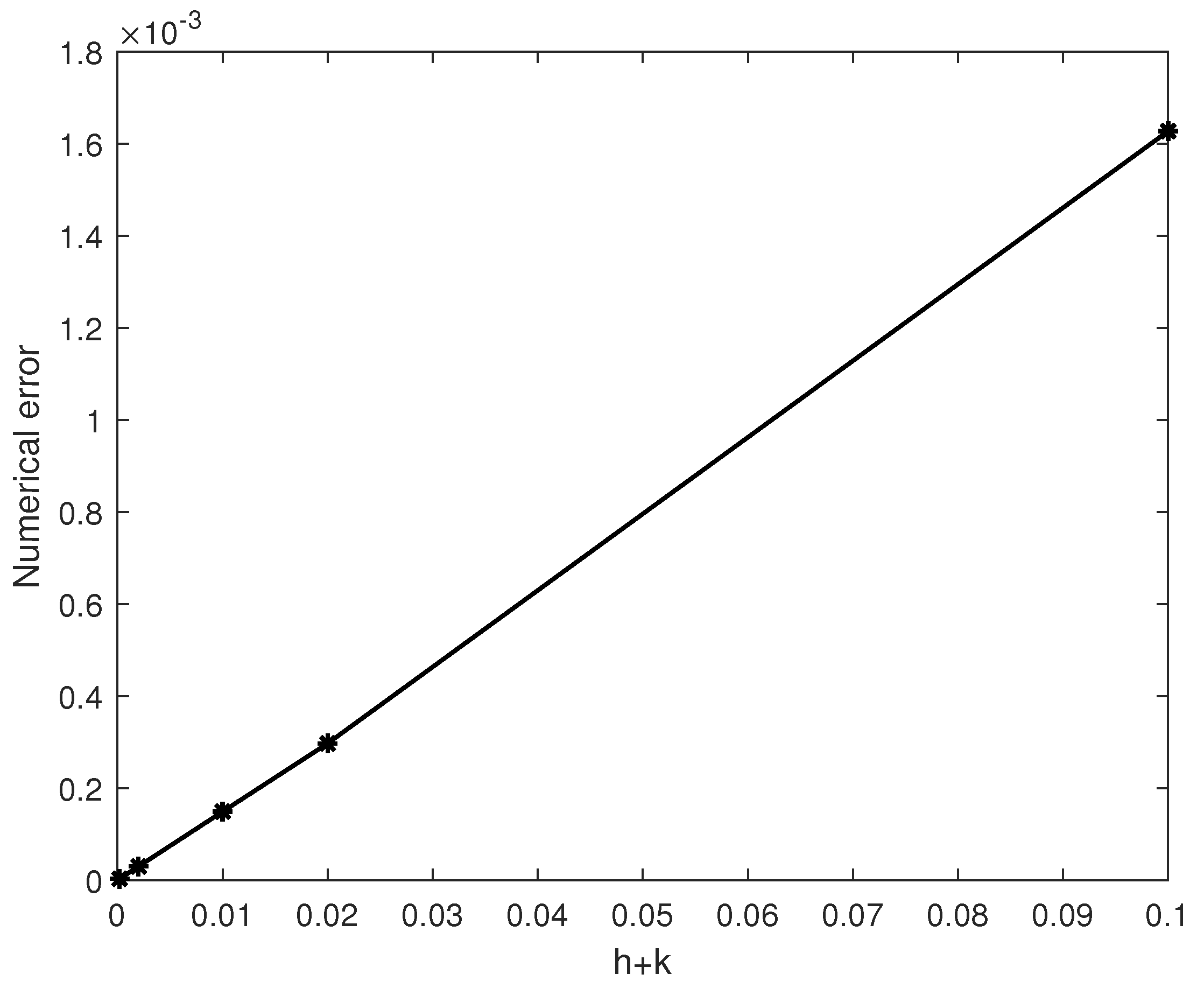
In this paper, we have studied, from the numerical point of view, several porous-thermoelastic problems assuming that the inertia effects are negligible (and so, the problems became quasi-static). As an example, we have focused on the study of the quasi-static porous-thermoelastic problem where the thermal law was modeled by the classical Fourier law. By using the implicit Euler scheme and the finite element method to discretize both the time derivatives and spatial variable, fully discrete approximations have been introduced. A discrete stability property and a priori error estimates have been proved, and the linear convergence has been deduced under some adequate additional regularity. Finally, we have provided some numerical simulations to show the numerical convergence of the algorithm in 
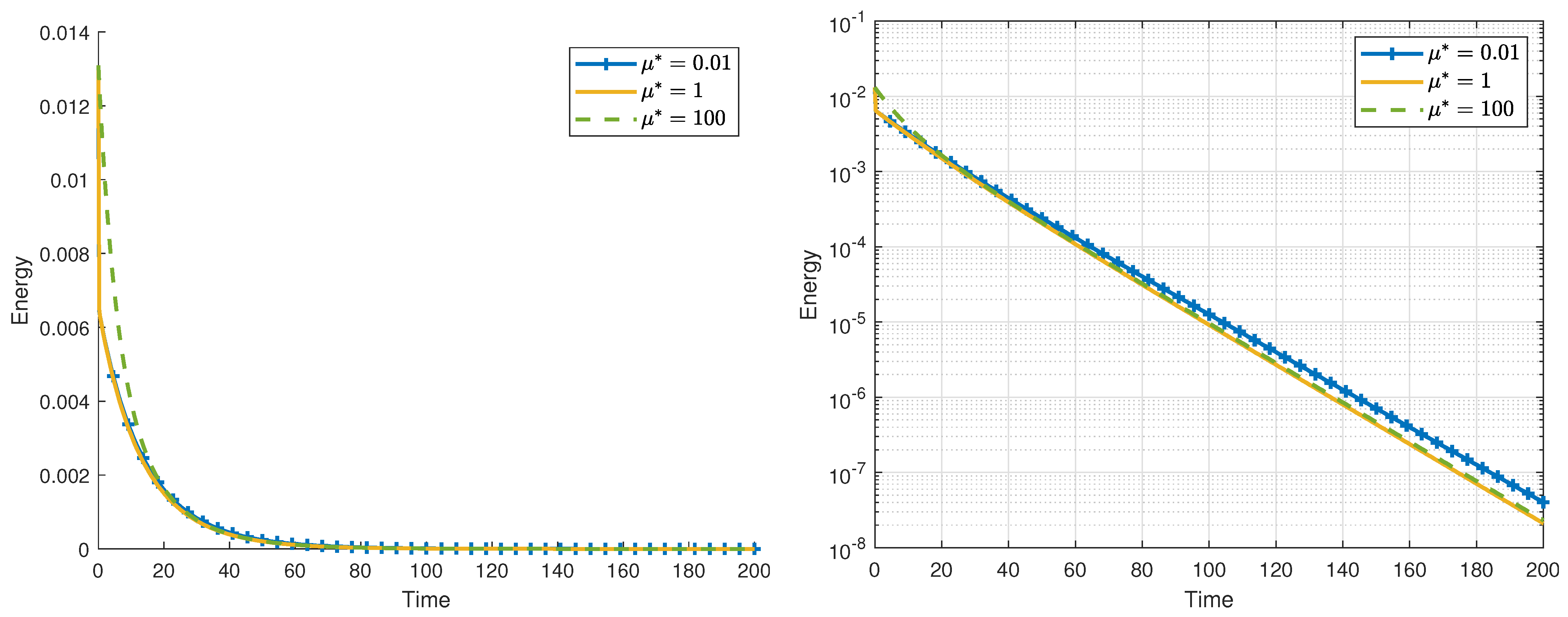
Section 4.1, where the linear convergence seems to be achieved. Then, in Section 4.2 a parametric study has been performed with respect to dissipative parameters μ * and κ * 
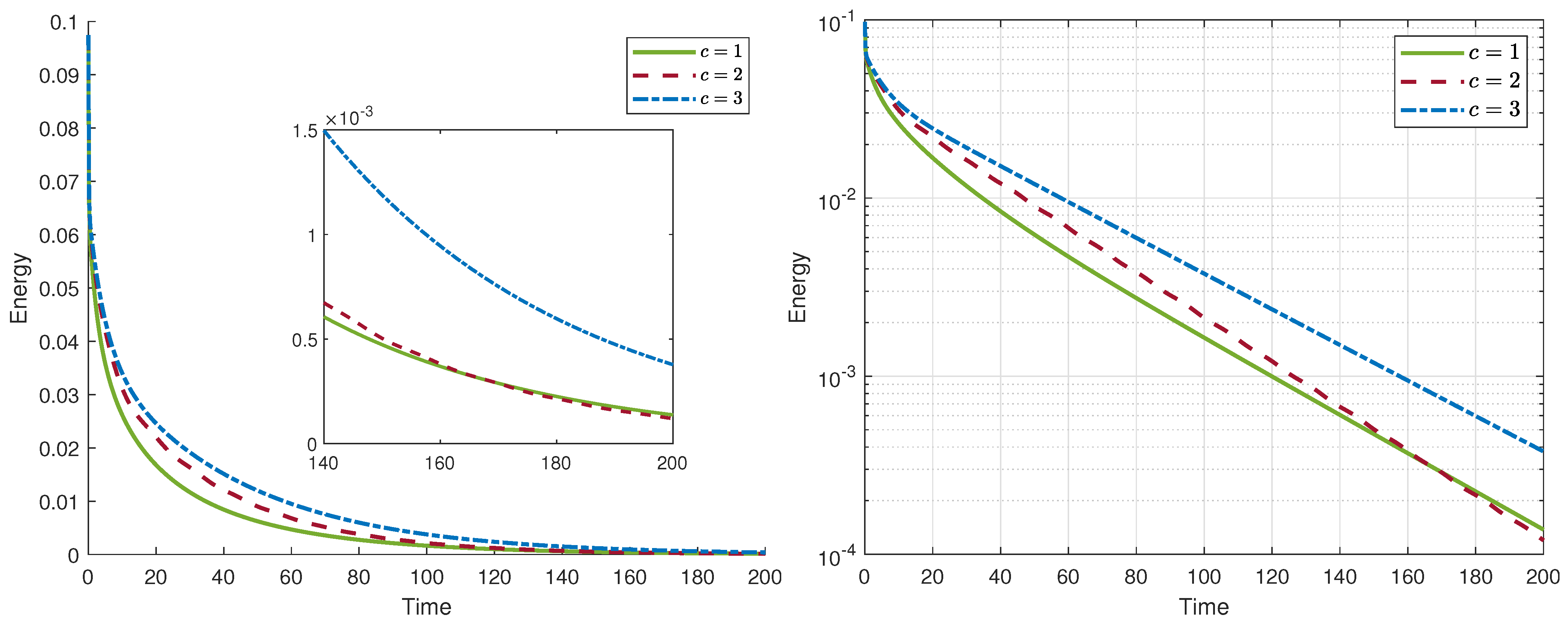
. Finally, the problem involving the so-called type II thermal law has been considered. A detailed analysis on some constitutive coefficients, as suggested in [22], has been shown.
At this time, the lack of experimental results does not allow to show which model is closer to reality. Both models behave similarly from a numerical point of view. In addition, the performance and complexity is similar in both cases. Therefore, the selection of the most appropriate model will depend on the specific application.

Author Contributions

Conceptualization, J.B. and J.R.F.; methodology, J.R.F.; software, J.B. and J.A.L.-C.; validation, J.B., J.R.F. and J.A.L.-C.; formal analysis, J.B. and J.R.F.; investigation, J.B., J.R.F. and J.A.L.-C.; resources, J.A.L.-C.; writing—original draft preparation, J.B. and J.R.F.; writing—review and editing, J.B., J.R.F. and J.A.L.-C.; supervision, J.R.F.; funding acquisition, J.R.F. All authors have read and agreed to the published version of the manuscript.

Funding

This research was funded by Ministerio de Ciencia, Innovación y Universidades grant number PGC2018-096696-B-I00 (FEDER, UE).

Institutional Review Board Statement

Not applicable.

Informed Consent Statement

Not applicable.

Data Availability Statement

Not applicable.

Conflicts of Interest

The authors declare no conflict of interest.

References

  1. Cosserat, E.; Cosserat, F. Théorie des Corps Déformables; A. Hermann et Fils: Paris, France, 1909. [Google Scholar]
  2. Cowin, S.C.; Nunziato, J.W. Linear elastic materials with voids. J. Elast. 1983, 13, 125–147. [Google Scholar] [CrossRef]
  3. Nunziato, J.W.; Cowin, S.C. A nonlinear theory of elastic materials with voids. Arch. Ration. Mech. Anal. 1979, 72, 175–201. [Google Scholar] [CrossRef]
  4. Casas, P.; Quintanilla, R. Exponential stability in thermoelasticity with microtemperatures. Int. J. Eng. Sci. 2005, 43, 33–47. [Google Scholar] [CrossRef] [Green Version]
  5. Feng, B. Uniform decay of energy for a porous thermoelastic system with past history. Appl. Anal. 2018, 97, 210–229. [Google Scholar] [CrossRef]
  6. Feng, B.; Apalara, T.A. Optimal decay for a porous elasticity system with memory. J. Math. Anal. Appl. 2019, 470, 1108–1128. [Google Scholar] [CrossRef]
  7. Leseduarte, M.C.; Magaña, A.; Quintanilla, R. On the time decay of solutions in porous-thermo-elasticity of type II. Discret Contin. Dyn. Syst. Ser. B 2010, 13, 375–391. [Google Scholar] [CrossRef]
  8. Pamplona, P.X.; Muñoz-Rivera, J.E.; Quintanilla, R. On the decay of solutions for porous-elastic systems with history. J. Math. Anal. Appl. 2011, 379, 682–705. [Google Scholar] [CrossRef]
  9. Santos, M.L.; Almeida Júnior, D.S. On the porous-elastic system with Kelvin–Voigt damping. J. Math. Anal. Appl. 2017, 445, 498–512. [Google Scholar] [CrossRef]
  10. Bazarra, N.; Fernández, J.R. Numerical analysis of a contact problem in poro-thermoelasticity with microtemperatures. Z. Angew. Math. Mech. 2018, 98, 1190–1209. [Google Scholar] [CrossRef]
  11. Bazarra, N.; Fernández, J.R.; Leseduarte, M.C.; Magaña, A.; Quintanilla, R. On the linear thermoelasticity with two porosities: Numerical aspects. Int. J. Numer. Anal. Model. 2020, 17, 172–194. [Google Scholar]
  12. Fernández, J.R.; Magaña, A.; Masid, M.; Quintanilla, R. Analysis for the strain gradient theory of porous thermoelasticity. J. Comput. Appl. Math. 2019, 345, 247–268. [Google Scholar] [CrossRef]
  13. Fernández, J.R.; Masid, M. Numerical analysis of a thermoelastic diffusion problem with voids. Int. J. Numer. Anal. Model. 2017, 14, 153–174. [Google Scholar]
  14. Fernández, J.R.; Masid, M. A porous thermoelastic problem: An a priori error analysis and computational experiments. Appl. Math. Comput. 2017, 305, 117–135. [Google Scholar] [CrossRef]
  15. Fernández, J.R.; Masid, M. A porous thermoviscoelastic mixture problem: Numerical analysis and computational experiments. Appl. Anal. 2018, 97, 1074–1093. [Google Scholar] [CrossRef]
  16. Green, A.E.; Naghdi, P.M. A unified procedure for construction of theories of deformable media. I. Classical continuum physics, II. Generalized continua, III. Mixtures of interacting continua. Proc. R. Soc. Lond. A 1995, 448, 335–377, 379–388. [Google Scholar]
  17. Mosconi, M. A variational approach to porous elastic voids. Z. Angew. Math. Phys. 2005, 56, 548–558. [Google Scholar] [CrossRef]
  18. Aouadi, M. Spatial stability for the quasi-static problem in thermoelastic diffusion theory. Acta Appl. Math. 2009, 106, 307–323. [Google Scholar] [CrossRef]
  19. Baiz, O.; Benaissa, H.; El Moutawakil, D.; Fakhar, R. Variational and numerical analysis of a quasistatic thermo-electro-visco-elastic frictional contact problem. Z. Angew. Math. Mech. 2019, 99, e201800138. [Google Scholar] [CrossRef]
  20. Magaña, A.; Quintanilla, R. On the time decay of solutions in porous-elasticity with quasi-static microvoids. J. Math. Anal. Appl. 2007, 331, 617–630. [Google Scholar] [CrossRef] [Green Version]
  21. Scarpetta, E.; Svanadze, M. Uniqueness theorems in the quasi-static theory of thermoelasticity for solids with double porosity. J. Elast. 2015, 120, 67–86. [Google Scholar] [CrossRef]
  22. Magaña, A.; Quintanilla, R. Decay of quasi-static porous-thermo-elastic waves. Z. Angew. Math. Phys. 2021, 72, 125. [Google Scholar] [CrossRef]
  23. Ciarlet, P.G. Basic error estimates for elliptic problems. In Handbook of Numerical Analysis; Ciarlet, P.G., Lions, J.L., Eds.; CRC Press: Boca Raton, FL, USA, 1993; Volume II, pp. 17–351. [Google Scholar]
  24. Campo, M.; Fernández, J.R.; Kuttler, K.L.; Shillor, M.; Viaño, J.M. Numerical analysis and simulations of a dynamic frictionless contact problem with damage. Comput. Methods Appl. Mech. Eng. 2006, 196, 476–488. [Google Scholar] [CrossRef]
Figure 1. Numerical convergence of the algorithm.
Mathematics 09 01436 g001
Figure 2. Evolution of the energy in natural (left) and semi-log (right) scales.
Mathematics 09 01436 g002
Figure 3. Evolution of the energy in natural (left) and semi-log (right) scales.
Mathematics 09 01436 g003
Figure 4. Evolution of the energy in natural (left) and semi-log (right) scales. In the case where c = 2 the decay velocity is expected to be higher because J κ = c δ .
Mathematics 09 01436 g004
Table 1. Numerical errors ( × 100 ).
h k 1 × 10 1 5 × 10 2 1 × 10 2 5 × 10 3 1 × 10 3 1 × 10 4
1 × 10 1 0.4148640.3389630.2957580.2921940.2897810.289303
5 × 10 2 0.282320.1627340.08319130.07712220.07355690.0729751
1 × 10 2 0.2721360.1416340.02971240.01521794.4344 × 10 3 3.00054 × 10 3
5 × 10 3 0.2721910.1416610.02958190.01490513.10211 × 10 3 8.39197 × 10 4
1 × 10 3 0.2722130.1416790.02958410.01489462.99667 × 10 3 3.01503 × 10 4
1 × 10 4 0.2722140.1416790.02958470.01489512.99693 × 10 3 3.00113 × 10 4
Publisher’s Note: MDPI stays neutral with regard to jurisdictional claims in published maps and institutional affiliations.

