
On Self-Interference Cancellation and Non-Idealities Suppression in Full-Duplex Radio Transceivers


Abstract
:1. Introduction
1.1. Related Work
1.2. Contributions
- Three RF/analog SIC techniques, i.e., CSI, GALL filter and Kautz filter for SI cancellation to level below the receiver’s thermal noise floor or sensitivity level.
- A digital SIC technique i.e., Kalman filter for residual SI cancellation.
- Linearization techniques for the suppression of the transceiver’s component (LNA, PA, IQ mixer) non idealities, i.e.,
- ➢
- BAFF and BA algorithm for IQ mixer imbalance
- ➢
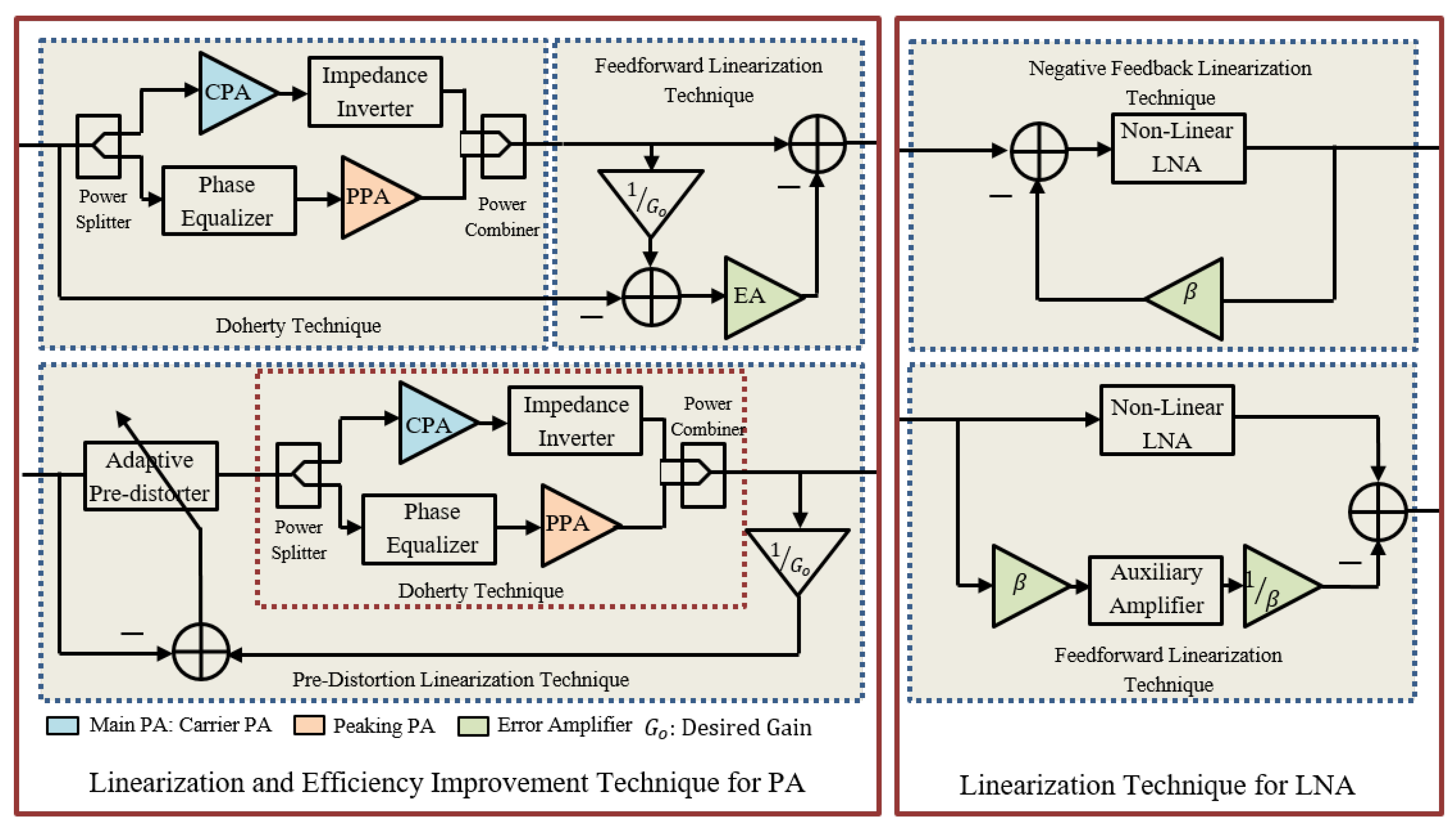
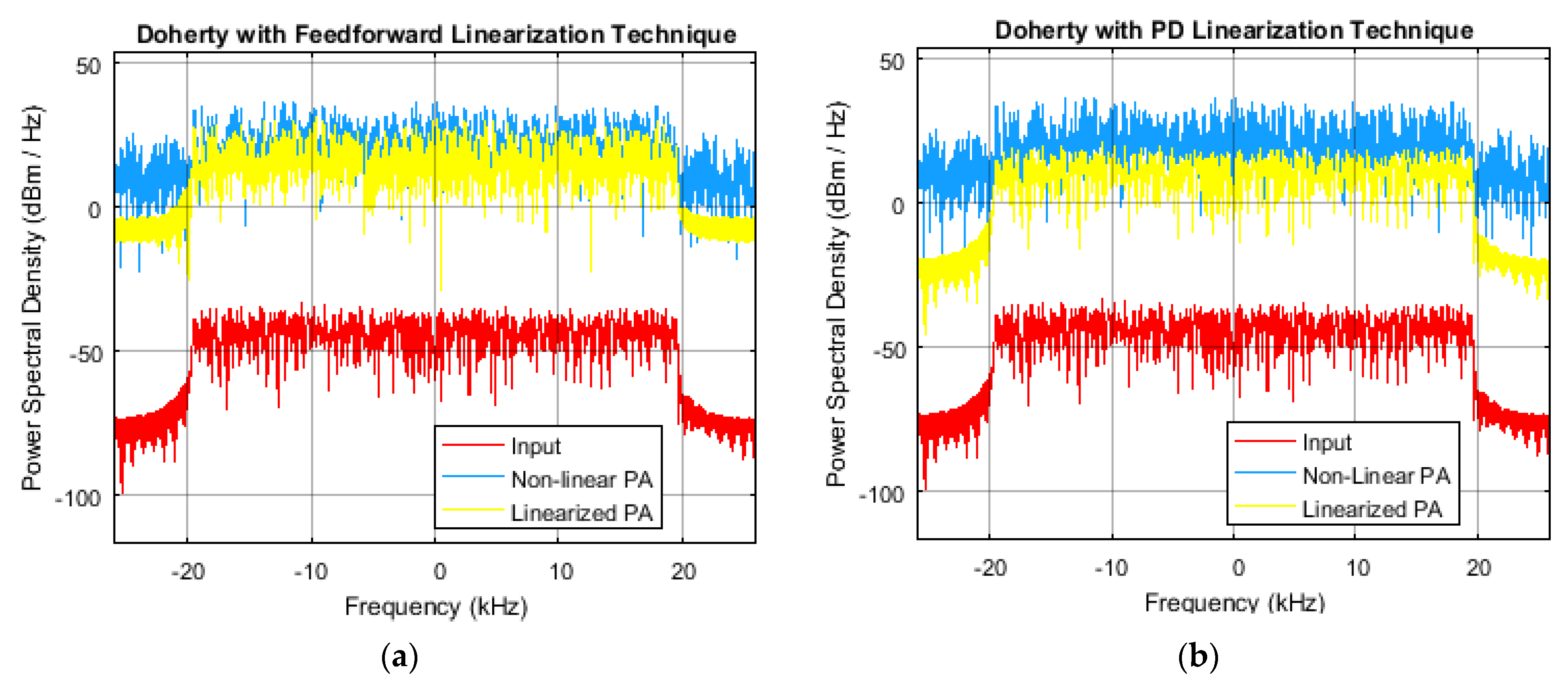
- Doherty amplifier technique with feedforward linearization technique and pre-distortion linearization technique for the linearization of PA
- ➢
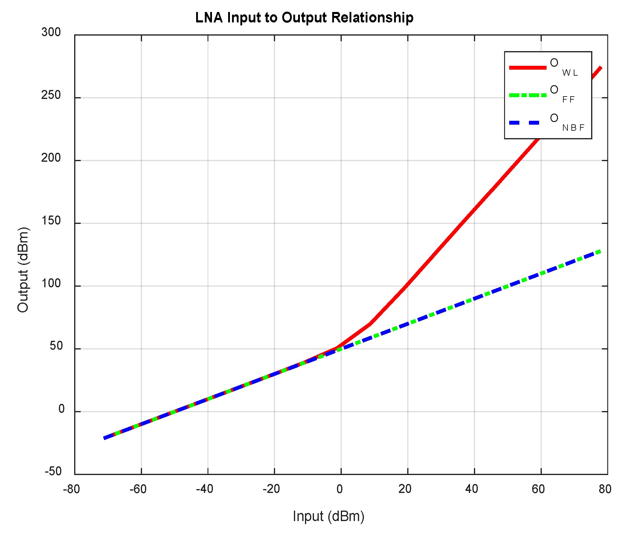
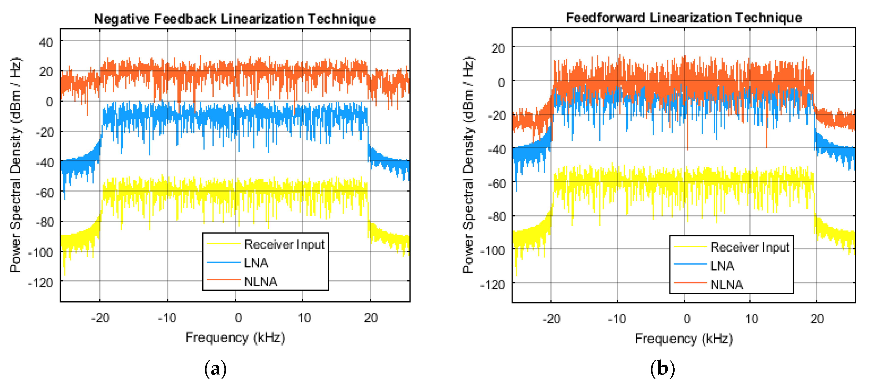
- Negative feedback and feedforward linearization technique for LNA.
1.3. Organization of the Paper
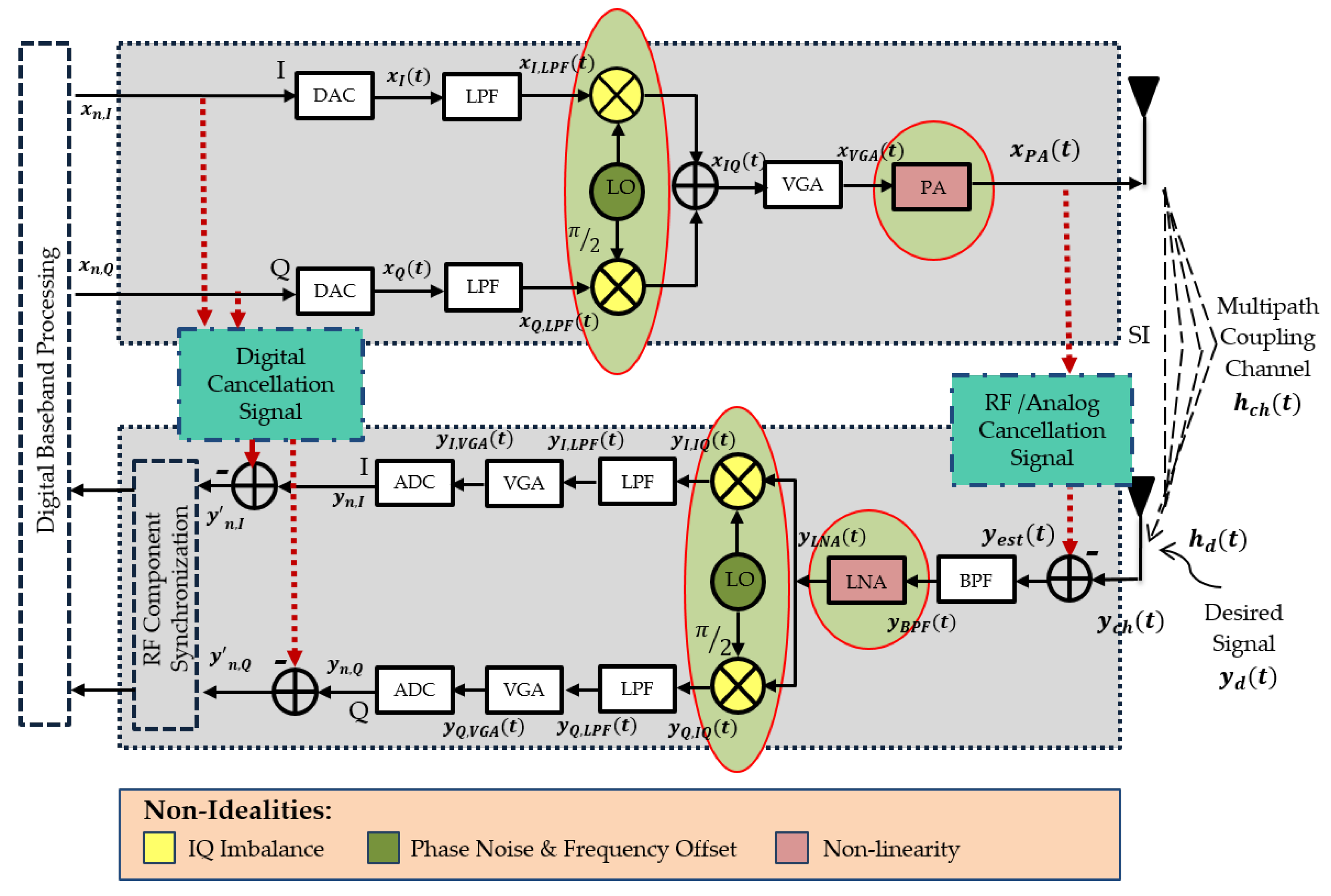
2. Proposed System Model and Techniques
2.1. Transceiver’s Components Linearization
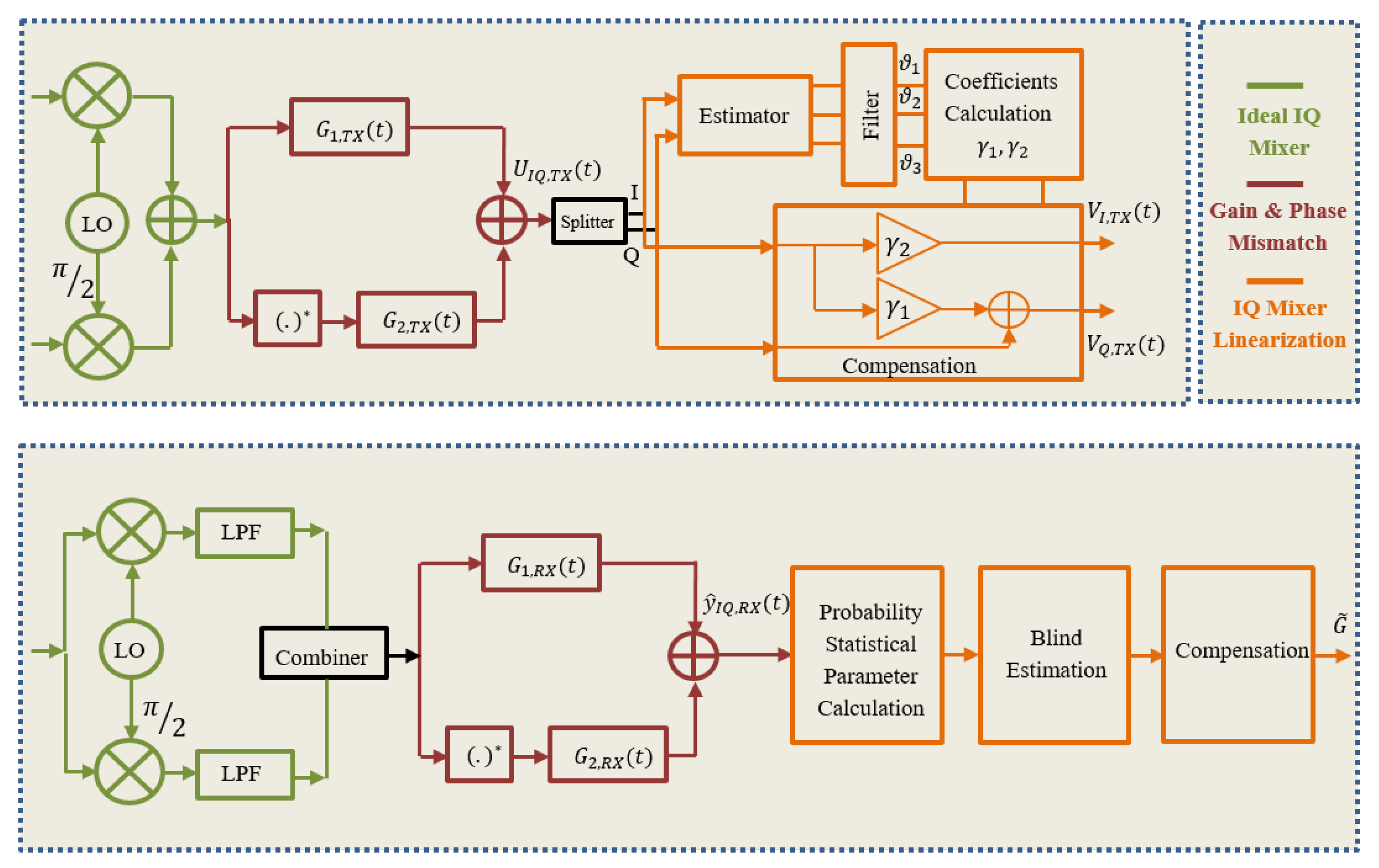
2.1.1. IQ Mixer Linearization
Tx: Blind Adaptive Feedforward Algorithm (BAFF)
Rx: Blind Algorithm (BA)
2.1.2. PA and LNA Linearization
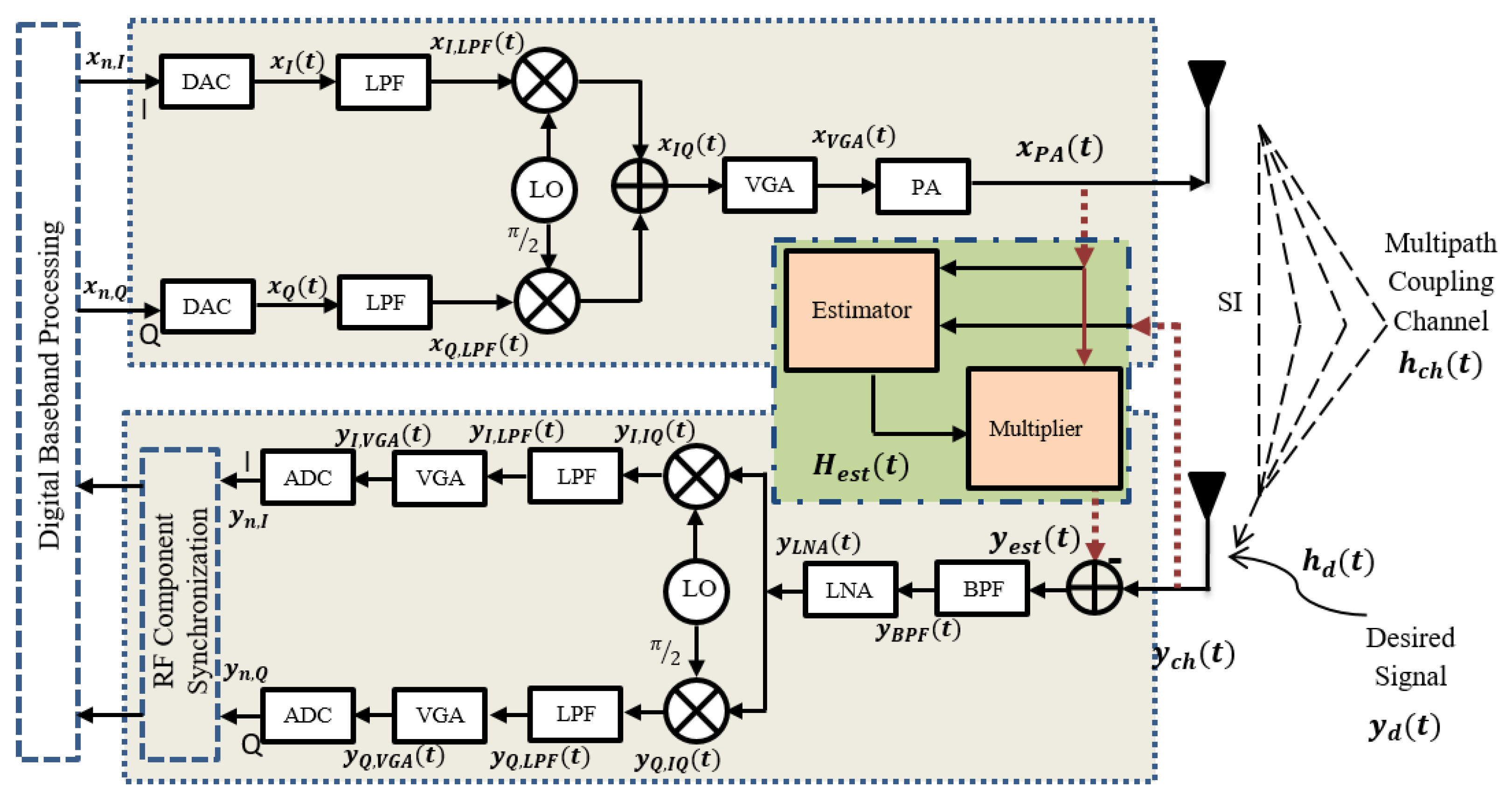
2.2. SI Cancellation Techniques
2.2.1. Analog/RF SI Cancellation Techniques
Channel State Information (CSI)
Channel State Information at Rx (CSIR)
Blind Estimation
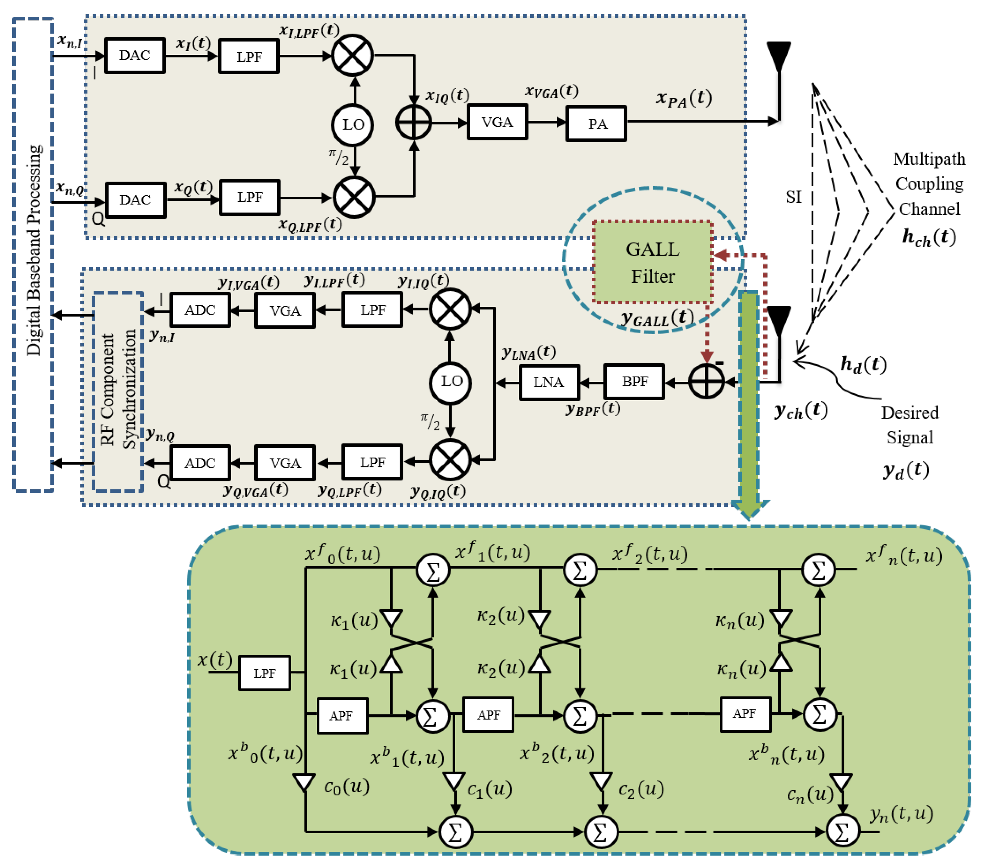
GALL Filter
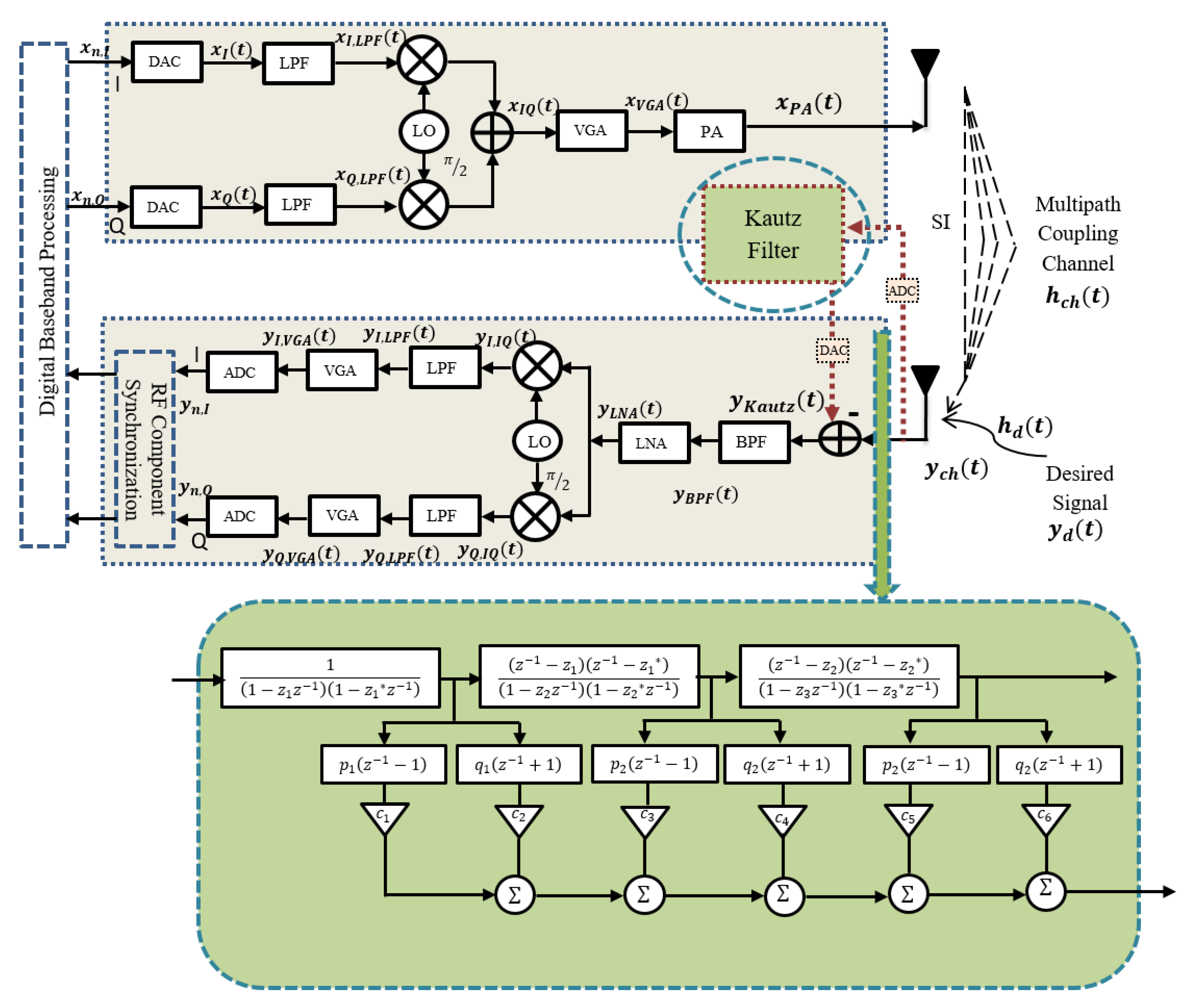
Kautz Filter
2.2.2. Digital SI Cancellation Techniques
Kalman Filter
- (i)
- Prediction stage:
- (ii)
- Updating stage:
3. Results and Discussion
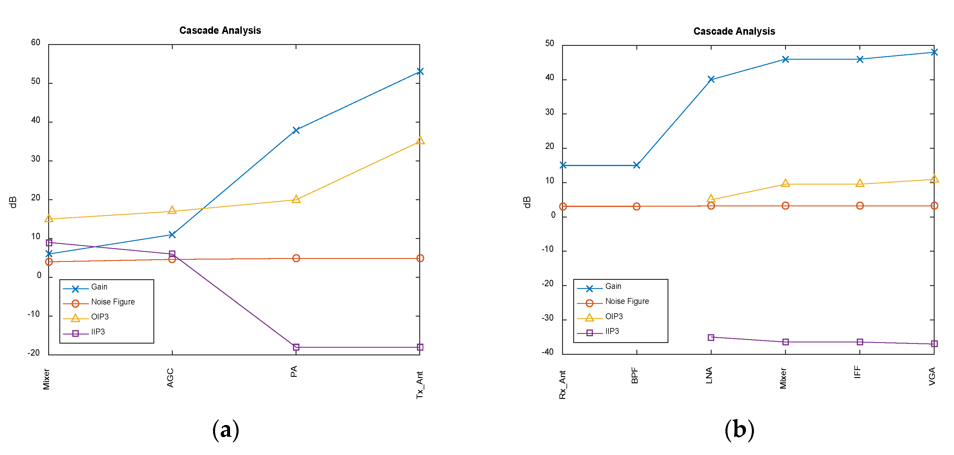
3.1. Link Budget Analysis
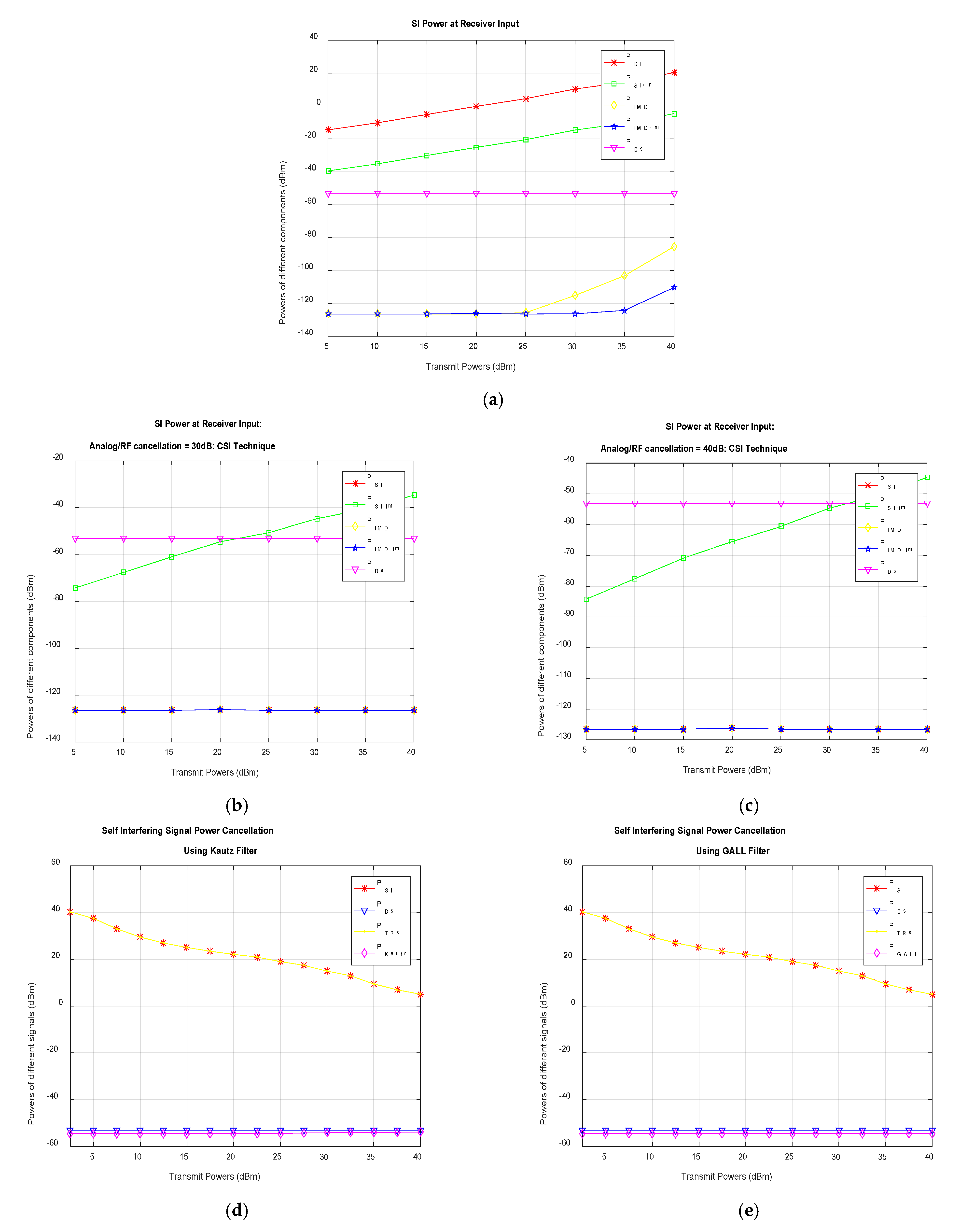
3.2. Power Level of Different Components of SI. Signal After RF/Analog SI Cancellation
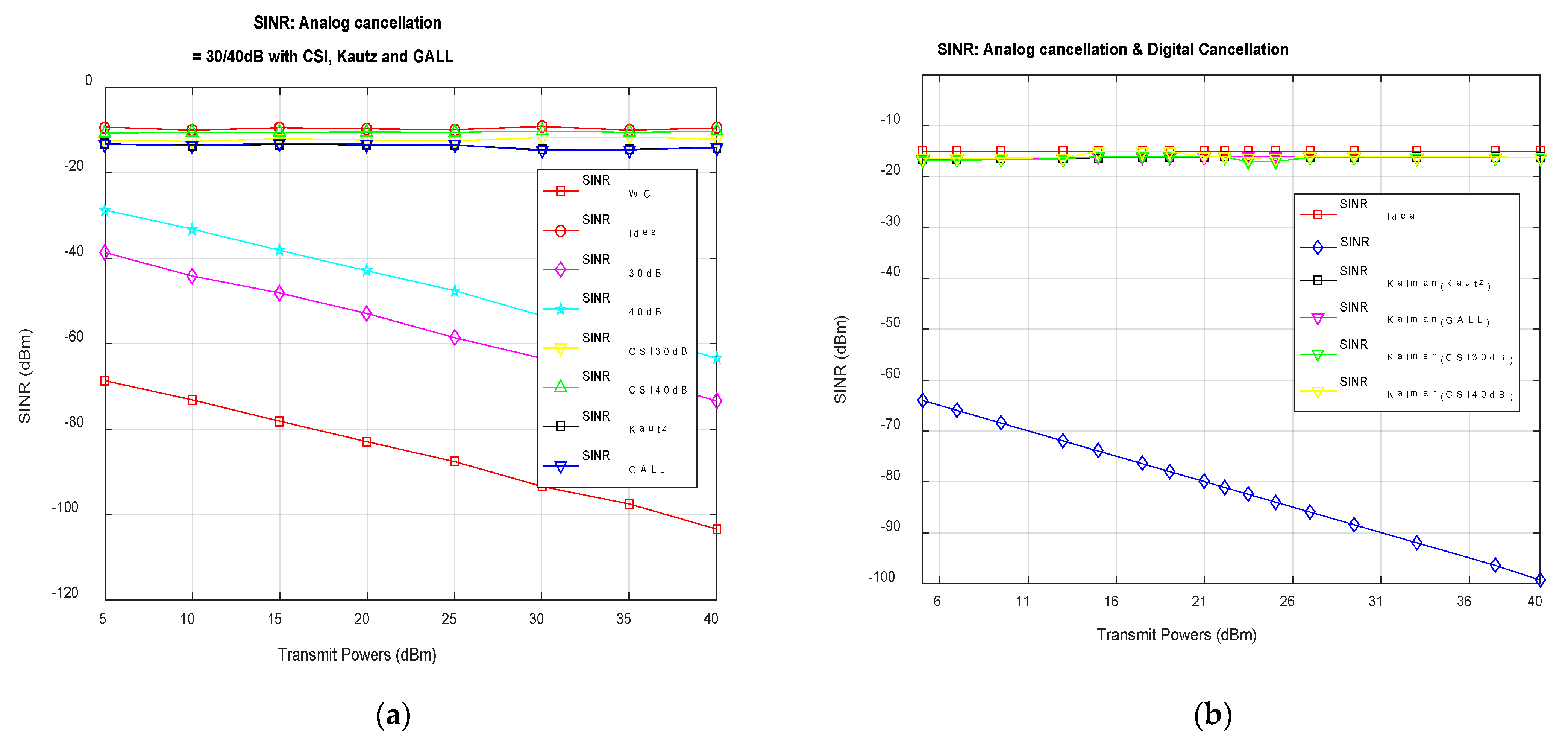
3.3. SINR
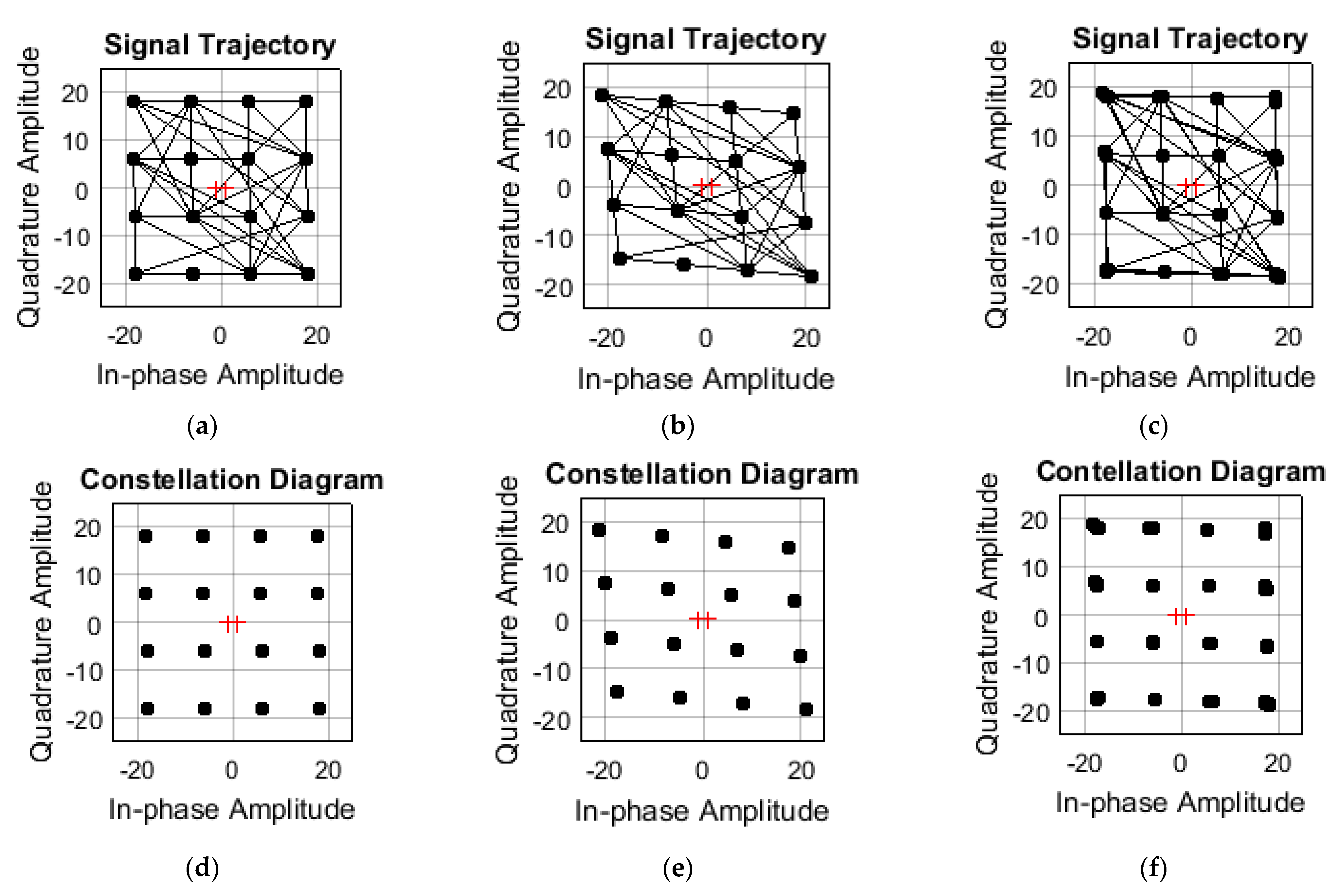
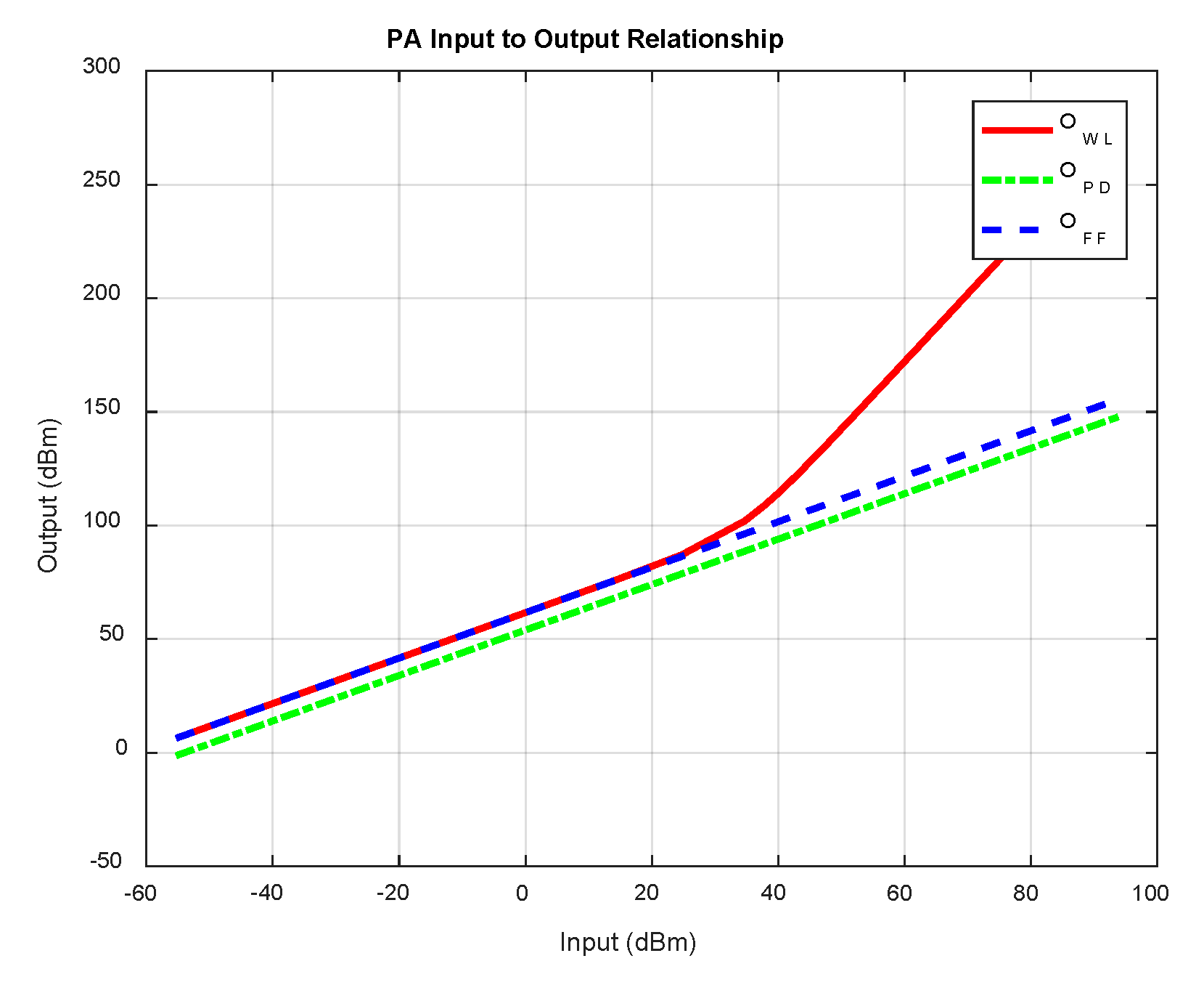
3.4. Linearization
4. Conclusions
Author Contributions
Funding
Institutional Review Board Statement
Informed Consent Statement
Data Availability Statement
Conflicts of Interest
Nomenclature
| Power of direct component | |
| Power of image component | |
| Power of intermediate distortion component | |
| Power of image component of IMD | |
| Power of desired Signal | |
| Total power at the receiver input | |
| Power after applying analog/RF cancellation using Kautz filter | |
| Power after applying analog/RF cancellation using GALL filter | |
| SINR without any cancellation technique | |
| SINR with 30 dB of antenna cancellation | |
| SINR with 40 dB of antenna cancellation | |
| SINR with CSI and 30 dB antenna cancellation | |
| SINR with CSI and 40 dB antenna cancellation | |
| SINR after Kautz filter implementation | |
| SINR after GALL filter implementation | |
| SINR after Kautz filter with Kalman filter implementation | |
| SINR after GALL filter with Kalman filter implementation | |
| SINR after CSI and 30 dB antenna cancellation with Kalman filter implementation | |
| SINR after CSI and 40 dB antenna cancellation with Kalman filter implementation | |
| The output of a non-linear amplifier | |
| The output of PA after PD technique | |
| The output of PA after FF technique | |
| The output of PA after NFB technique | |
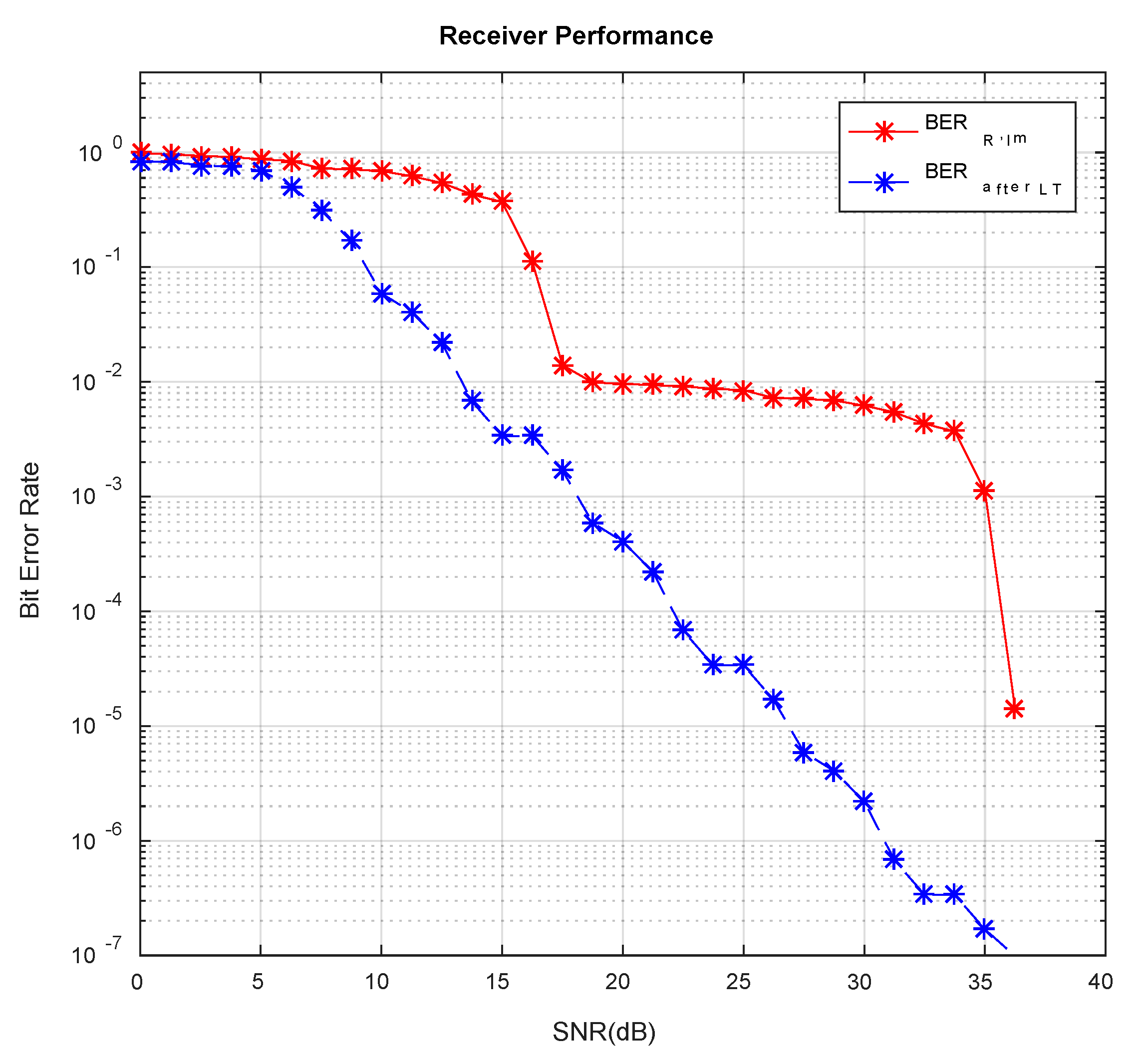
| BER in the presence of receiver front end impairments | |
| BER after applying linearization techniques to receiver front end components |
References
- Choi, J.I.; Jain, M.; Srinivasan, K.; Levis, P.; Katti, S. Achieving Single Channel, Full Duplex Wireless Communication. In Proceedings of the Sixteenth Annual International Conference on Mobile Computing and Networking (MobiCom’10), Houston, TX, USA, 12–14 November 2019; Association for Computing Machinery: New York, NY, USA, 2010; pp. 1–12. [Google Scholar] [CrossRef]
- Weeraddana, P.C.; Codreanu, M.; Latvaaho, M.; Ephremides, A. On the effect of self-interference cancelation in multi-hop wireless networks. EURASIP J. Wirel. Commun. Netw. 2010, 2010, 1–10. [Google Scholar] [CrossRef] [Green Version]
- Korpi, D.; Riihonen, T.; Syrjala, V.; Anttila, L.; Valkama, M.; Wichman, R. Full-duplex transceiver system calculations: Analysis of ADC and linearity challenges. IEEE Trans. Wirel. Commun. 2014, 13, 3821–3836. [Google Scholar] [CrossRef] [Green Version]
- Knox, M.E. Single antenna full-duplex communications using a common carrier. In Proceedings of the WAMICON 2012 IEEE Wireless and Microwave Technology Conference, Cocoa Beach, FL, USA, 15–17 April 2012; pp. 1–6. [Google Scholar]
- Cox, C.; Ackerman, E. Demonstration of a single-aperture, full-duplex communication system. In Proceedings of the 2013 IEEE Radio and Wireless Symposium, Austin, TX, USA, 20–23 January 2013; pp. 148–150. [Google Scholar]
- Jain, M.; Choi, J.I.; Kim, T.; Bharadia, D.; Seth, S.; Srinivasan, K.; Levis, P.; Katti, S.; Sinha, P. Practical, real-time, full-duplex wireless. In Proceedings of the 17th Annual International Conference on Mobile Computing and Networking, Las Vegas, NV, USA, 19–23 September 2011; pp. 301–312. [Google Scholar]
- Sahai, A.; Patel, G.; Sabharwal, A. Pushing the limits of full-duplex: Design and real-time implementation. arXiv 2011, arXiv:1107.0607. [Google Scholar]
- Duarte, M.; Sabharwal, A. Full-duplex wireless communications using off-the-shelf radios: Feasibility and first results. In Proceedings of the 2010 Conference Record of the Forty-Fourth Asilomar Conference on Signals, Systems, and Computers, Pacific Grove, CA, USA, 7–10 November 2010; pp. 1558–1562. [Google Scholar]
- Phunganmgern, N.; Uthansakul, P.; Uthansakul, M. Digital and RF interference cancellation for single-channel full-duplex transceiver using a single antenna. In Proceedings of the 2013 10th International Conference on Electrical Engineering/Electronics, Computer, Telecommunications, and Information Technology, Krabi, Thailand, 15–17 May 2013; pp. 1–5. [Google Scholar]
- Anderson, C.R.; Krislmamoorthy, S.; Ran Son, C.G.; Lemon, T.J.; Newhall, W.G.; Kummetz, T.; Reed, J.H. Antenna isolation, wideband multi-path propagation measurements, and interference mitigation for on-frequency repeaters. In Proceedings of the IEEE Southeast Conference, Greensboro, NC, USA, 26–29 March 2004; pp. 110–114. [Google Scholar]
- Carroll, A.; Heiser, G. An analysis of power consumption in a smartphone. In Proceedings of the USENIX Annual Technical Conference, Boston, MA, USA, 23–25 June 2010; p. 21. [Google Scholar]
- Singh, V.; Gadre, A.; Kumar, S. Full Duplex Radios: Are we there yet? In Proceedings of the 19th ACM Workshop on Hot Topics in Networks, Virtual Event, New York, NY, USA, 4–6 November 2020; pp. 117–124. [Google Scholar]
- Nguyen, B.C.; Thang, N.N.; Tran, X.M.; Dung, L.T. Impacts of imperfect channel state information, transceiver hardware, and self-interference cancellation on the performance of full-duplex mimo relay system. Sensors 2020, 20, 1671. [Google Scholar] [CrossRef] [PubMed] [Green Version]
- Alves, H.; Riihonen, T.; Suraweera, H.A. Full-Duplex Communications for Future Wireless Networks; Springer: Singapore, 2020. [Google Scholar]
- Sahai, A.; Patel, G.; Sabharwal, A. Asynchronous full-duplex wireless. In Proceedings of the 2012 Fourth International Conference on Communication Systems and Networks (COMSNETS 2012), Bangalore, India, 3–7 January 2012; pp. 1–9. [Google Scholar]
- Tsakalaki, E.P.; Alrabadi, O.N.; Tatomirescu, A.; De Carvalho, E.; Pedersen, G.F. Antenna cancellation for simultaneous cognitive radio communication and sensing. In Proceedings of the 2013 International Workshop on Antenna Technology (iWAT), Karlsruhe, Germany, 4–6 March 2013; pp. 215–218. [Google Scholar]
- Choi, J.I.; Hong, S.; Jain, M.; Katti, S.; Levis, P.; Mehlman, J. Beyond full-duplex wireless. In Proceedings of the 2012 Conference Record of the Forty-Sixth Asilomar Conference on Signals, Systems, and Computers (ASILOMAR), Pacific Grove, CA, USA, 4–7 November 2012; pp. 40–44. [Google Scholar]
- Hong, S.S.; Mehlman, J.; Katti, S. Picasso: Flexible RF and spectrum slicing. ACM SIGCOMM Comput. Commun. Rev. 2012, 42, 37–48. [Google Scholar] [CrossRef]
- Duarte, M. Full-Duplex Wireless: Design, Implementation, and Characterization. Ph.D. Dissertation, Rice University, Houston, TX, USA, 2012. [Google Scholar]
- He, Z.; Shao, S.; Shen, Y.; Qing, C.; Tang, Y. Performance analysis of RF self-interference cancellation in full-duplex wireless communications. IEEE Wirel. Commun. Lett. 2014, 3, 405–408. [Google Scholar] [CrossRef]
- Duarte, M.; Dick, C.; Sabharwal, A. Experiment-driven characterization of full-duplex wireless systems. IEEE Trans. Wirel. Commun. 2012, 11, 4296–4307. [Google Scholar] [CrossRef] [Green Version]
- Yang, B.; Dong, Y.; Yu, Z.; Zhou, J. An RF self-interference cancellation circuit for the full-duplex wireless communications. In Proceedings of the 2013 International Symposium on Antennas and Propagation, Nanjing, China, 23–25 October 2013; pp. 1048–1051. [Google Scholar]
- Bharadia, D.; Katti, S. Fast-forward: Fast and constructive full-duplex relays. ACM SIGCOMM Comput. Commun. Rev. 2014, 44, 199–210. [Google Scholar] [CrossRef]
- Riihonen, T.; Mathecken, P.; Wichman, R. Effect of oscillator phase noise and processing delay in full-duplex OFDM repeaters. In Proceedings of the 2012 Conference Record of the Forty-Sixth Asilomar Conference on Signals, Systems, and Computers (ASILOMAR), Pacific Grove, CA, USA, 4–7 November 2012; pp. 1947–1951. [Google Scholar]
- Dine, T.; Krishnaswamy, H. AT/R antenna pair with polarization-based reconfigurable wideband self-interference cancellation for simultaneous transmit and receive. In Proceedings of the IEEE MTT-S International Microwave Symposium, Phoenix, AZ, USA, 17–22 May 2015; pp. 1–4. [Google Scholar]
- Debaillie, B.; van den Broek, D.J.; Lavin, C.; van Liempd, B.; Klumperink, E.A.; Palacios, C.; Craninckx, J.; Nauta, B.; Parssinen, A. Analog/RF solutions enabling compact full-duplex radios. IEEE J. Sel. Areas Commun. 2014, 32, 1662–1673. [Google Scholar] [CrossRef]
- Khojastepour, M.A.; Sundaresan, K.; Rangarajan, S.; Zhang, X.; Barghi, S. The case for antenna cancellation for scalable full-duplex wireless communications. In Proceedings of the 10th ACM Workshop on Hot Topics in Networks, Cambridge, MA, USA, 14–15 November 2011; pp. 1–6. [Google Scholar]
- Hu, J.; Di, B.; Liao, Y.; Bian, K.; Song, L. Hybrid MAC protocol design and optimization for full duplex Wi-Fi networks. IEEE Trans. Wirel. Commun. 2018, 17, 3615–3630. [Google Scholar] [CrossRef]
- Alexandris, K.; Balatsoukas-Stimming, A.; Burg, A. Measurement-based characterization of residual self-interference on a full-duplex MIMO testbed. In Proceedings of the IEEE 8th Sensor Array and Multichannel Signal Processing Workshop (SAM), A Coruna, Spain, 22–25 June 2014; pp. 329–332. [Google Scholar]
- Xu, Q.; Quan, X.; Zhang, Z.; Tang, Y.; Shen, Y. Analysis and experimental verification of digital self-interference cancelation for co-time co-frequency full-duplex LTE. Int. J. Signal Process. Image Process. Pattern Recognit. 2014, 7, 299–312. [Google Scholar] [CrossRef]
- Razavi, B. RF Microelectronics, 2nd ed.; Prentice Hall: Hoboken, NJ, USA, 2012. [Google Scholar]
- Bliss, D.W.; Hancock, T.; Schniter, P. Hardware phenomenological effects on cochannel full-duplex MIMO relay performance. In Proceedings of the 2012 Conference Record of the Forty-Sixth Asilomar Conference on Signals, Systems, and Computers (ASILOMAR), Pacific Grove, CA, USA, 4–7 November 2012; pp. 34–39. [Google Scholar]
- Sahai, A.; Patel, G.; Dick, C.; Sabharwal, A. Understanding the impact of phase noise on active cancellation in wireless full-duplex. In Proceedings of the 2012 Conference Record of the Forty-Sixth Asilomar Conference on Signals, Systems, and Computers (ASILOMAR), Pacific Grove, CA, USA, 4–7 November 2012; pp. 29–33. [Google Scholar]
- Sytjala, V.; Valkama, M.; Anttila, L.; Riihonen, T.; Korpi, D. Analysis of oscillator phase noise effects on self-interference cancellation in full-duplex OFDM radio transceivers. IEEE Trans. Wirel. Commun. 2014, 13, 2977–2990. [Google Scholar] [CrossRef] [Green Version]
- Ahmed, E.; Eltawil, A.M.; Sabharwal, A. Self-interference cancellation with phase noise induced ICI suppression for full-duplex systems. In Proceedings of the 2013 IEEE Global Communications Conference (GLOBECOM), Atlanta, GA, USA, 9–13 December 2013; pp. 3384–3388. [Google Scholar]
- Sahai, A.; Patel, G.; Dick, C.; Sabharwal, A. On the impact of phase noise on active cancelation in wireless full-duplex. IEEE Trans. Veh. Technol. 2013, 62, 4494–4510. [Google Scholar] [CrossRef]
- Ahmed, E.; Eltawil, A.M.; Sabharwal, A. Rate gain region and design tradeoffs for full-duplex wireless communications. IEEE Trans. Wirel. Commun. 2013, 12, 3556–3565. [Google Scholar] [CrossRef] [Green Version]
- Anttila, L. Digital front-end signal processing with widely linear signal models in radio devices. Ph.D. Dissertation, Tampere University of Technology, Tampere, Finland, 14 October 2011. [Google Scholar]
- Korpi, D.; Anttila, L.; Syrjala, V.; Valkama, M. Widely linear-digital self-interference cancellation in direct-conversion full-duplex transceiver. IEEE J. Sel. Areas Commun. 2014, 32, 1674–1687. [Google Scholar] [CrossRef] [Green Version]
- Li, S.; Murch, R.D. Full-duplex wireless communication using transmitter output-based echo cancellation. In Proceedings of the 2011 IEEE Global Telecommunications Conference—GLOBECOM 2011, Houston, TX, USA, 5–9 December 2011; pp. 1–5. [Google Scholar]
- Tsai, J.H.; Chen, Y.J.; Lai, Y.F.; Shen, M.H.; Huang, P.C. A 14-bit 200MS/s current-steering DAC achieving over 82dB SFDR with digitally assisted calibration and dynamic matching techniques. In Proceedings of the Technical Program of 2012 VLSI Design, Automation and Test, Hsinchu, Taiwan, 23–25 April 2012; pp. 1–4. [Google Scholar]
- Everett, E.; Sahai, A.; Sabharwal, A. Passive self-interference suppression for full-duplex infrastructure nodes. IEEE Trans. Wirel. Commun. 2014, 13, 680–694. [Google Scholar] [CrossRef] [Green Version]
- Ahmed, E.; Eltawil, A.M.; Sabharwal, A. Self-interference cancellation with nonlinear distortion suppression for full-duplex systems. In Proceedings of the 2013 Asilomar Conference on Signals, Systems and Computers, Pacific Grove, CA, USA, 3–6 November 2013; pp. 1199–1203. [Google Scholar]
- Bensmida, S.; Morris, K.; Lees, J.; Wright, P.; Benedikt, J.; Tasker, P.J.; Beach, M.; McGeehan, J. Power amplifier memoryless pre-distortion for 3GPP LTE application. In Proceedings of the 2009 European Microwave Conference (EuMC), Rome, Italy, 29 September–1 October 2009; pp. 1433–1436. [Google Scholar]
- Riihonen, T.; Wichman, R. Analog and digital self-interference cai1cellation in full-duplex MIMO-OFDM transceivers with limited resolution in A/D conversion. In Proceedings of the 2012 Conference Record of the Forty-Sixth Asilomar Conference on Signals, Systems, and Computers (ASILOMAR), Pacific Grove, CA, USA, 4–7 November 2012; pp. 45–49. [Google Scholar]
- Komatsu, K.; Miyaji, Y.; Uehara, H. Iterative Nonlinear Self-Interference Cancellation for In-Band Full-Duplex Wireless Communications Under Mixer Imbalance and Amplifier Nonlinearity. IEEE Trans. Wirel. Commun. 2020, 19, 4424–4438. [Google Scholar]
- Evolved Universal Terrestrial Radio Access (E-UTRA). User Equipment (UE) Radio Access Capabilities ‘TR 36.306’; 3rd Generation Partnership Project (3GPP): Phoenix, AZ, USA, January 2015; Available online: https://portal.3gpp.org/desktopmodules/Specifications/SpecificationDetails.aspx?specificationId=2434 (accessed on 1 March 2021).
- De Witt, J.J.; Van Rooyen, G.J. Novel IQ imbalance and offset compensation techniques for quadrature mixing radio transceivers. In Proceedings of the Southern African Telecommunication Networks Applications Conference (SATNAC), Stellenbosch, South Africa, 3–6 September; pp. 1–6.
- Panda, S.; Panigrahi, S.P.; Neema, D.D.; Mishra, R.; Sahu, M.K.; Sahu, H.S.; Panda, N.; Singh, M. A Novel Approach to Blind I/Q Mismatch and Carrier Offset Compensation. J. Signal Inf. Process. 2011, 2, 18. [Google Scholar] [CrossRef] [Green Version]
- Nguyen, T.H.; Scalart, P.; Joindot, M.; Gay, M.; Bramerie, L.; Peucheret, C.; Carer, A.; Simon, J.C.; Sentieys, O. Joint simple blind IQ imbalai1ce compensation and adaptive equalization for 16-QAM optical communications. In Proceedings of the 2015 IEEE International Conference on Communications (ICC), London, UK, 8–12 June 2015; pp. 4913–4918. [Google Scholar]
- Windisch, M.; Fettweis, G. On the performance of standard-independent I/Q imbalance compensation in OFDM direct-conversion receivers. In Proceedings of the 13th European Signal Processing Conference, Antalya, Turky, 4–8 September 2005; pp. 1–5. [Google Scholar]
- Mailand, M.; Richter, R.; Jentschel, H.J. Blind IQ-imbalance compensation using iterative inversion for arbitrary direct conversion receivers. In Proceedings of the 14th IST Mobile and Wireless Communications Summit, Dresden, Germany, 19–23 June 2005; pp. 1–5. [Google Scholar]
- Özen, M.; Gustafsson, D.; Buisman, K.; Fager, C. A Doherty power amplifier design method for improved efficiency and linearity. IEEE Trans. Microw. Theory Tech. 2016, 64, 4491–4504. [Google Scholar]
- Son, J.; Kim, I.; Moon, J.; Lee, J.; Kim, B. A highly efficient asymmetric Doherty power amplifier with a new output combining circuit. In Proceedings of the 2011 IEEE International Conference on Microwaves, Communications, Antennas and Electronic Systems (COMCAS 2011), Tel Aviv, Israel, 7–9 November 2011; pp. 1–4. [Google Scholar]
- Moon, J.; Kim, J.; Kim, J.; Kim, I.; Kim, B. Efficiency Enhancement of Doherty Amplifier Through Mitigation of the Knee Voltage Effect. IEEE Trans. Microw. Theory Tech. 2011, 59, 143–152. [Google Scholar] [CrossRef]
- Pasricha, R.; Sharma, S. Modeling of a Power Amplifier for Digital pre-distortion Applications using Simplified Complex Memory Polynomial. Appl. Math. Inf. Sci. 2013, 7, 1519. [Google Scholar] [CrossRef]
- Jiang, H.; Wilford, P.A. Digital pre-distortion for power amplifiers using separable functions. IEEE Trans. Signal Process. 2010, 58, 4121–4130. [Google Scholar] [CrossRef] [Green Version]
- Breed, G.; Director, E. An overview of common techniques for power amplifier linearization. IEEE Microw. Wirel. Comp. Lett. 2008, 18, 673. [Google Scholar]
- Tung, Y.C.; Han, S.; Chen, D.; Shin, K.G. Vulnerability and protection of channel state information in multiuser MIMO networks. In Proceedings of the 2014 ACM SIGSAC Conference on Computer and Communications Security, Scottsdale, AZ, USA, 3–7 November 2014; pp. 775–786. [Google Scholar]
- Sharma, M. Effective Channel State Information (CSI) Feedback for MIMO Systems in Wireless Broadband Communications. Ph.D. Thesis, Queensland University of Technology, Queensland, Australia, 2014. [Google Scholar]
- Cho, Y.S.; Kim, J.; Yang, W.Y.; Kang, C.G. MIMO-OFDM Wireless Communications with MATLAB; John Wiley and Sons: Hoboken, NJ, USA, 2010. [Google Scholar]
- Campi, M.; Leonardi, R.; Rossi, L.A. Generalized super-exponential method for blind equalization using Kautz filters. In Proceedings of the IEEE Signal Processing Workshop on Higher-Order Statistics (SPW-HOS ’99), Caesarea, Israel, 16 June 1999; pp. 107–111. [Google Scholar]
- e Silva, T.O. On the adaptation of the pole of Laguerre-lattice filters. In Proceedings of the 8th European Signal Processing Conference (EUSIPCO 1996), Trieste, Italy, 10–13 September 1996; pp. 1–4. [Google Scholar]
- Kim, S.W.; Park, Y.C.; Youn, D.H. A variable step-size filtered-x gradient adaptive lattice algorithm for active noise control. In Proceedings of the 2012 IEEE International Conference on Acoustics, Speech and Signal Processing (ICASSP), Kyoto, Japan, 25–30 March 2012; pp. 189–192. [Google Scholar]
- Dam, H.; Cantoni, A.; Nordholm, S.; Teo, K.L. Digital Laguerre filter design with maximum passband-to-stopband energy ratio subject to peak and group delay constraints. IEEE Trans. Circuits Syst. I Regul. Pap. 2006, 53, 1108–1118. [Google Scholar] [CrossRef]
- Paatero, T.; Karjalainen, M.; Harma, A. Modeling, and equalization of audio systems using Kautz filters. In Proceedings of the 2001 IEEE International Conference on Acoustics, Speech, and Signal Processing, Proceedings (Cat. No. 01CH37221). Salt Lake City, UT, USA, 7–11 May 2001; pp. 3313–3316. [Google Scholar]
- Kurt, T.; Lerbour, R.; Le Helloco, Y.; Breton, B. Adaptive Kalman filtering for local mean power estimation in mobile communications. In Proceedings of the IEEE Vehicular Technology Conference (VTC Fall), Montreal, QC, Canada, 25–28 September 2006; pp. 1–4. [Google Scholar]
- Lekshmi, B.; Susan, S.; Apren, D.T. Channel Estimation with Extended Kalman Filter for Fading Charmels. Int. J. Electron. Commun. Comput. Technol. 2013, 3, 9–13. [Google Scholar]
- Ayesha, A.; Chaudhry, S.M. Self-Interference Cancellation for Full-Duplex Radio Transceivers Using Extended Kalman Filter. Natl. Acad. Sci. Lett. 2020, 7, 631–634. [Google Scholar] [CrossRef]
- Mohinder, S.; Angus, P. Kalman Filtering: Theory and Practice Using Matlab; John Wiley and Sons: Hoboken, NJ, USA, 2001. [Google Scholar]
- Anderson, B.D.; Moore, J.B. Optimal Filtering; Dover Publication, Inc.: Mineola, NY, USA, 2012. [Google Scholar]
- Chen, L.; Mercorelli, P.; Liu, S. A Kalman estimator for detecting repetitive disturbances. In Proceedings of the 2005, American Control Conference, Portland, OR, USA, 8–10 June 2005; pp. 1631–1636. [Google Scholar]
- Faragher, R. Understanding the basis of the Kalman filter via a simple and intuitive derivation [lecture notes]. IEEE Signal Process. Mag. 2012, 29, 128–132. [Google Scholar] [CrossRef]
- Duarte, M.; Sabharwal, A.; Aggarwal, V.; Jana, R.; Ramakrishnan, K.K.; Rice, C.W.; Shankaranarayanan, N.K. Design and characterization of a full-duplex multiantenna system for WiFi networks. IEEE Trans. Veh. Technol. 2014, 3, 1160–1177. [Google Scholar] [CrossRef] [Green Version]
- Heino, M.; Korpi, D.; Huusari, T.; Rodriguez, E.A.; Venkatasubramanian, S.; Riihonen, T.; Anttila, L.; Icheln, C.; Haneda, K.; Wichman, R. Recent advances in antenna design and interference cancellation algorithms for in-band full duplex relays. IEEE Commun. Mag. 2015, 5, 91–101. [Google Scholar] [CrossRef]
- Huusari, T.; Choi, Y.S.; Liikkanen, P.; Korpi, D.; Talwar, S.; Valkama, M. Wideband self-adaptive RF cancellation circuit for full-duplex radio: Operating principle and measurements. In Proceedings of the 81st Vehicular Technology Conference (VTC Spring), Glasgow, UK, 11–14 May 2015; pp. 1–7. [Google Scholar]
- Tamminen, J.; Turunen, M.; Korpi, D.; Huusari, T.; Choi, Y.-S.; Talwar, S.; Valkama, M. Digitally-controlled RF self-interference canceller for full-duplex radios. In Proceedings of the 24th European Signal Processing Conference (EUSIPCO), Budapest, Hungary, 29 August–2 September 2016; pp. 783–787. [Google Scholar]
- Khaledian, S.; Farzami, F.; Smida, B.; Erricolo, D. Inherent self-interference cancellation at 900 MHz for in-band full-duplex applications. In Proceedings of the IEEE 19th Wireless and Microwave Technology Conference (WAMICON), Sand Key, FL, USA, 9–10 April 2018; pp. 1–4. [Google Scholar]
- Kiayani, A.; Waheed, M.Z.; Anttila, L.; Abdelaziz, M.; Korpi, D.; Syrjala, V.; Kosunen, M.; Stadius, K.; Ryynänen, J.; Valkama, M. Adaptive nonlinear RF cancellation for improved isolation in simultaneous transmit–receive systems. IEEE Trans. Microw. Theory Tech. 2018, 5, 2299–2312. [Google Scholar] [CrossRef]
- Islam, M.A.; Smida, B. A comprehensive self-interference model for single-antenna full-duplex communication systems. In Proceedings of the IEEE International Conference on Communications (ICC 2019), Shanghai, China, 20–24 May 2019; pp. 1–7. [Google Scholar]
- Martínez, M.F.; Alonso, F.J.M.; Valcarce, R.L. Solving Self-Interference Issues in a Full-Duplex Radio Transceiver. Multidiscip. Digit. Publ. Inst. Proc. 2019, 1, 35. [Google Scholar]
- Singh, V.; Mondal, S.; Gadre, A.; Srivastava, M.; Paramesh, J.; Kumar, S. Millimeter-wave full duplex radios. In Proceedings of the 26th Annual International Conference on Mobile Computing and Networking (MobiCom ’20), London, UK, 21–25 September 2020; pp. 1–14. [Google Scholar]


| Parameters | Values |
|---|---|
| Modulation Scheme | 16 QAM |
| Number of Sub-carriers | 64 |
| Number of Data sub-carriers | 48 |
| Symbol Time | 3.2 µs |
| Guard Interval or CP Duration | 25% of symbol length |
| Parameters | Values |
|---|---|
| Bandwidth | 20 MHz |
| Receiver thermal noise floor | −103.0 dBm |
| Sensitivity | −88.9 dBm |
| Receiver noise figure | 4.1 dB |
| Noise power | −174 dBm/Hz |
| Power at receiver | −88.9 dBm |
| Transmit power | 5 to 40 dBm |
| Antenna separation | 30 dB and 40 dB |
| Carrier frequency | 2 GHz |
| Component | Gain (dB) | IIP2 (dBm) | IIP3 (dBm) | NF (dB) |
|---|---|---|---|---|
| IQ Mixer (Tx and Rx) | 6 | 50 | 15 | 4 |
| PA | 27 | - | 20 | 5 |
| LNA | 25 | - | 5 | 4.1 |
| VGA | 1–51 | 50 | 20 | 4 |
| IQ Mixer IRR (dB) (Tx and Rx) | 13 | - | - | - |
| PA memory length | 6 | - | - | - |
| ADC | Bits | 12 | - | - |
| P-P voltage range | 4.5 V | - | - | |
| PAPR | 10 dB | - | - |
| Techniques | Results | Reference Papers | ||||
|---|---|---|---|---|---|---|
| Analog/RF SIC | Digital SIC | Linearization Techniques (LT) | Analog/RF SIC | Digital SIC | ||
| Auxiliary path (consisting of DAC, IQ, PA and RF attenuator) | Gain factor | - | 74 dB | [17] | ||
| Robust algorithm known as SINC interpolation | LS algorithm | - | 60 dB | Residual linear components by 50 dB | [74] | |
| Non-linear components by 20 dB. | ||||||
| Hybrid model enables SI cancellation near to receiver noise floor up to 110 dB | ||||||
| One tap filter depicting the delay, phase and attenuation of main coupling path | LS estimator | - | 30 dB & 20 dB | Linear Model: 25 dB | [39] | |
| Widely Linear Model: 35 or 50 dB | ||||||
| Passive isolation (special antenna design) | - | - | Passive isolation: 60–70 dB | - | [75] | |
| 100 dB of overall self-interference suppression | ||||||
| Presents a novel RF circuit architecture | - | - | 100 MHz waveform bandwidth: 41 dB total cancellation | - | [76] | |
| 20 MHz carrier bandwidth: 60 dB total cancellation | ||||||
| Digitally controlled RF self-interference canceller structure | - | - | More than 40 dBs of active RF cancellation gain up to 80 MHz instantaneous waveform bandwidths | - | [77] | |
| Used a shared antenna and a circulator, an adjustable impedance mismatch terminal (IMT) circuit at the antenna interface is added for cancellation of SI | - | - | 40 dB | - | [78] | |
| Block-adaptive Learning algorithm through decorrelation for RF cancellation | - | - | 54 dB | - | [79] | |
| Assumed 15 dB circulator isolation with variable RF cancellation | Orthogonalization of the design matrix using QR decomposition | - | As low as 50 dB | [80] | ||
| Hybrid multi-stage cancellation system, consisting of an analog cancellation setup at RF frequencies following the so-called Stanford architecture | Base-band digital cancellation i. LMS (Least Mean Square) ii. APA (Affine Projection Algorithm) methods | - | Up to 80 dB of power interference cancellation can be achieved with a full-duplex OFDM scheme | [81] | ||
| Nonlinear signal reconstruction and cancellation with post-distortion, least-squares method for channel estimation | - | Iteratively estimation of coefficients (IQ Imbalance, PA and LNA) using Newton’s method & discrete Fourier transform | Approximately 50 dB | [46] | ||
| Antenna cancellation, self-reflector and develop custom Arduino code for updating the weights for RF cancellation | Develop custom Arduino code for updating the weights in in-house chip using SPI | - | 58 dB | 26 dB | [82] | |
| Total of 84 dB | ||||||
| Assumed 30 dB and 40 dB antenna isolation | Extended Kalman Filter (EKF) | - | - | 40–45 dB | Our previous work [69] | |
| KALMAN Filter |
|
| 40–45 dB | PROPOSED WORK | |
| Proposed model results. (Assumed antenna isolation of 30 dB & 40 dB) |
|
* If EKF (our own previous work) is used for digital SIC, SIC of 115–130 dB. | ||||
Publisher’s Note: MDPI stays neutral with regard to jurisdictional claims in published maps and institutional affiliations. |
© 2021 by the authors. Licensee MDPI, Basel, Switzerland. This article is an open access article distributed under the terms and conditions of the Creative Commons Attribution (CC BY) license (https://creativecommons.org/licenses/by/4.0/).
Share and Cite
Ayesha, A.; Rahman, M.; Haider, A.; Majeed Chaudhry, S. On Self-Interference Cancellation and Non-Idealities Suppression in Full-Duplex Radio Transceivers. Mathematics 2021, 9, 1434. https://doi.org/10.3390/math9121434
Ayesha A, Rahman M, Haider A, Majeed Chaudhry S. On Self-Interference Cancellation and Non-Idealities Suppression in Full-Duplex Radio Transceivers. Mathematics. 2021; 9(12):1434. https://doi.org/10.3390/math9121434
Chicago/Turabian StyleAyesha, Areeba, MuhibUr Rahman, Amir Haider, and Shabbir Majeed Chaudhry. 2021. "On Self-Interference Cancellation and Non-Idealities Suppression in Full-Duplex Radio Transceivers" Mathematics 9, no. 12: 1434. https://doi.org/10.3390/math9121434