Estimating the Quadratic Form x^TA^−mx for Symmetric Matrices: Further Progress and Numerical Computations

Abstract

In this paper, we study estimates for quadratic forms of the type $x^T{A}^{-m}x$, $m\in \mathbb{N}$, for symmetric matrices. We derive a general approach for estimating this type of quadratic form and we present some upper bounds for the corresponding absolute error. Specifically, we consider three different approaches for estimating the quadratic form $x^T{A}^{-m}x$. The first approach is based on a projection method, the second is a minimization procedure, and the last approach is heuristic. Numerical examples showing the effectiveness of the estimates are presented. Furthermore, we compare the behavior of the proposed estimates with other methods that are derived in the literature.

1. Introduction

Let $A\in {\mathbb{R}}^{n\times n}$ be a given symmetric positive definite matrix and $x\in {\mathbb{R}}^n$. We are interested in estimating the quadratic forms of the type $x^T{A}^{-m}x$, $m\in \mathbb{N}$. Our main goal was to find an efficient and cheap approximate evaluation of the desired quadratic form without the direct computation of the matrix $A^{-m}$. As such, we revisited the approach for estimating the quadratic form $x^T{A}^{-1}x$, developed in [1], and extended it to the case of an arbitrary negative power of A.

The computation of quadratic forms is a mathematical problem with many applications. Indicatively, we refer to some usual applications.

• Statistics: The inverse of the covariance matrix, which is referred to as a precision matrix, usually appears in statistics. The covariance matrix reveals marginal correlations between the variables, whereas the precision matrix represents the conditional correlations between two data variables of the other variables [2]. The diagonal of the inverse of covariance matrices provides information about the quality of data in uncertainty quantification [3].
• Network analysis: The determination of the importance of the nodes of a graph is a major issue in network analysis. Information for these details can be extracted by the evaluation of the diagonal elements of the matrix ${(I_n-aA)}^{-1}$, where A is the adjacency matrix of the network, $0<a<{\displaystyle \frac{1}{\rho \left(A\right)}}$, and $\rho \left(A\right)$ is the spectral radius of A. This matrix is referred to as a resolvent matrix, see, for example, [4] and the references therein.
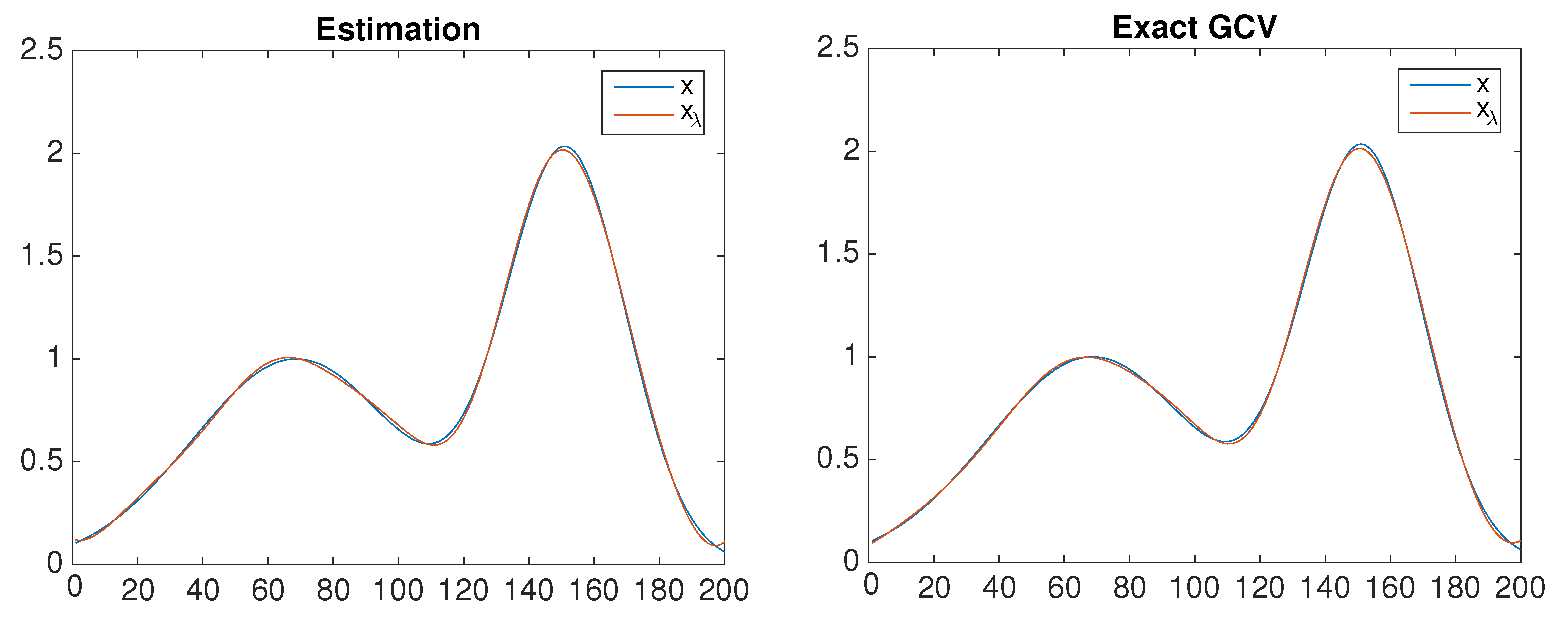
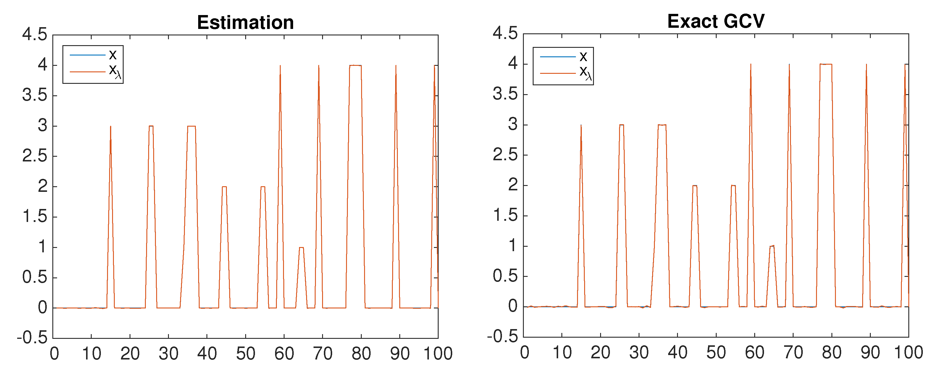
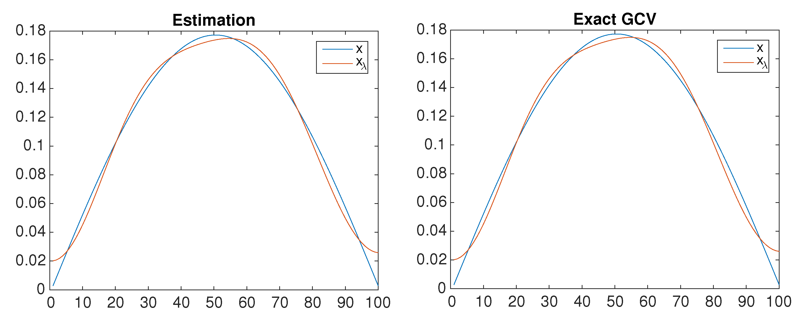
• Numerical analysis: Quadratic forms arise naturally in the context of the computation of the regularization parameter in Tikhonov regularization for solving ill-posed problems. In this case, the matrix has the form $A{A}^T+\lambda I_n$, $\lambda >0$. In the literature, many methods have been proposed for the selection of the regularization parameter $\lambda$, such as the discrepancy principle, cross-validation, generalized cross-validation (GCV), L-curve, and so forth; see, for an example, [5] (Chapter 15) and references therein. These methods involve quadratic forms of type $x^T{(A{A}^T+\lambda I_n)}^{-m}x$, with $m=1,2,3$.

In practice, exact computation of a quadratic form is often replaced using an estimate that is faster to evaluate. Regarding its numerous applications, the estimation of quadratic forms is an important practical problem that has been frequently studied in the literature. Let us indicatively refer to some well-known methods. A widely used method is based on Gaussian quadrature [5] (Chapter 7) and [6]. Moreover, extrapolation procedures have been proposed. Specifically, in [7], families of estimates for the bilinear form $x^T{A}^{-1}y$ for any invertible matrix, and in [8], families of estimates for the bilinear form $y^{*}f\left(A\right)x$ for a Hermitian matrix were developed.

In the present work, we consider alternative approaches to this problem. To begin, notice that the value of the quadratic form $(x,A^{-m}x)$ is proportional to the second power of the norm of x. Therefore, the task of estimating $(x,A^{-m}x)$ consists of two steps:

• Finding an $\alpha$ such that

  $$(x,A^{-m}x)\approx \alpha {\parallel x\parallel }^2.$$

  (1)
• Assessing the absolute error of the above estimate, i.e., determining a bound for the quantity

  $$\left|{\alpha \parallel x\parallel }^2-(x,A^{-m}x)\right|.$$

  (2)

In Section 2, we present the upper bounds for the absolute error (2) for any given $\alpha$. Section 3 is devoted to estimates of the value $\alpha$ in (1) using a projection method. In Section 4, we use bounds from Section 2 as a stepping stone for estimating $x^T{A}^{-m}x$ using the minimization method. A heuristic approach is outlined in Section 5. In Section 6, we briefly describe two methods that were used in previous studies, namely, an extrapolation approach and another one based on Gaussian quadrature. Section 7 is focused on adapting the proposed estimates to the case of the matrix of form $A{A}^T+\lambda I_n$. Numerical examples that illustrate the performance of the derived estimates are found in Section 8. We end this work with several concluding remarks in Section 9.

2. Bounds on the Error

In Proposition 1 below, we derive an upper bound on the error (2) for a given estimate ${\alpha \parallel x\parallel }^2$ of the quadratic form $x^T{A}^{-m}x$. The first three expressions for the bounds (UB1–UB3) are a direct generalization of a result from [1].

Proposition 1.

Let $A\in {\mathbb{R}}^{n\times n}$ be a symmetric positive definite matrix and $x\in {\mathbb{R}}^n$ and $est={\alpha \parallel x\parallel }^2$ be an estimate of the quadratic form $x^T{A}^{-m}x$. If we denote $b=\alpha A^{m}x-x$, the absolute error of the estimate $\left|{\alpha \parallel x\parallel }^2-(x,A^{-m}x)\right|$ is bounded from above by the following expressions:

UB1. 

${\displaystyle \frac{{\parallel x\parallel }^2\parallel b\parallel }{2\parallel A^{m}x\parallel }}\left({\kappa }^m+{\displaystyle \frac{1}{{\kappa }^m}}\right)$

UB2. 

${\displaystyle \frac{\parallel x\parallel ·{\parallel b\parallel }^2}{2\parallel A^{m}b\parallel }}\left({\kappa }^m+{\displaystyle \frac{1}{{\kappa }^m}}\right)$

UB3. 

${\displaystyle \frac{{\parallel x\parallel }^2{\parallel b\parallel }^2}{4\sqrt{x^T{A}^{m}x}·\sqrt{b^T{A}^{m}b}}}{\left({\kappa }^{m/2}+{\displaystyle \frac{1}{{\kappa }^{m/2}}}\right)}^2$

UB4. 

${\displaystyle \frac{\parallel x\parallel ·\parallel b\parallel }{{\lambda }_{min}^m}}$

UB5. 

For estimates satisfying ${\alpha \parallel x\parallel }^2\le (x,A^{-m}x)$, we have also the family of error bounds

$$\frac{{\parallel x\parallel }^2}{2\parallel A^{m}x\parallel ·\parallel A^{p}x\parallel }\left({\kappa }^m+\frac{1}{{\kappa }^m}\right)\sqrt{\parallel A^p{x\parallel }^2{\parallel b\parallel }^2-{(A^{p}x,b)}^2},$$

where$p\ge 0$can be chosen as any integer such that$\frac{(x,A^{p}x)}{(A^{m}x,A^{p}x)}<\alpha$.

Proof. 

• UB1.

The matrix $A^{-m}$ is symmetric because A is symmetric, and it holds that

$$|x^T{A}^{-m}b|=|(x,A^{-m}b)|=|(A^{-m}x,b)|\le \parallel A^{-m}x\parallel ·\parallel b\parallel ,$$

by the Cauchy–Schwarz inequality.

Moreover, we have

$$\parallel A^{-m}x\parallel =\sqrt{(A^{-m}x,A^{-m}x)}=\sqrt{(x,A^{-2m}x)}.$$

(3)

Using the Kantorovich inequality for the matrix $A^m$ and considering that ${\lambda }_{min}\left(A^{2m}\right)={\lambda }_{min}^{2m}$, ${\lambda }_{max}\left(A^{2m}\right)={\lambda }_{max}^{2m}$, we have

$$\begin{array}{cc}\hfill {\displaystyle \frac{{\left(x^{T}x\right)}^2}{\left(x^T{A}^{2m}x\right)\left(x^T{\left(A^{2m}\right)}^{-1}x\right)}}& \ge {\displaystyle \frac{4{\lambda }_{min}\left(A^{2m}\right){\lambda }_{max}\left(A^{2m}\right)}{{({\lambda }_{min}\left(A^{2m}\right)+{\lambda }_{max}\left(A^{2m}\right))}^2}}\hfill \\ \hfill \Rightarrow {\displaystyle \frac{{\parallel x\parallel }^4}{\left(x^T{A}^{2m}x\right)\left(x^T{A}^{-2m}x\right)}}& \ge {\displaystyle \frac{4{\lambda }_{min}^{2m}{\lambda }_{max}^{2m}}{{({\lambda }_{min}^{2m}+{\lambda }_{max}^{2m})}^2}}\hfill \\ \hfill \Rightarrow x^T{A}^{-2m}x& \le {\displaystyle \frac{{\parallel x\parallel }^4}{(x,A^{2m}x)}}{\displaystyle \frac{{({\lambda }_{min}^{2m}+{\lambda }_{max}^{2m})}^2}{4{\lambda }_{min}^{2m}{\lambda }_{max}^{2m}}}\hfill \\ \hfill \Rightarrow x^T{A}^{-2m}x& \le {\displaystyle \frac{{\parallel x\parallel }^4}{4\parallel A^m{x\parallel }^2}}{\left({\displaystyle \frac{{\lambda }_{min}^m}{{\lambda }_{max}^m}}+{\displaystyle \frac{{\lambda }_{max}^m}{{\lambda }_{min}^m}}\right)}^2={\displaystyle \frac{{\parallel x\parallel }^4}{4\parallel A^m{x\parallel }^2}}{\left({\displaystyle \frac{1}{{\kappa }^m}}+{\kappa }^m\right)}^2,\hfill \end{array}$$

where $\kappa ={\displaystyle \frac{{\lambda }_{max}}{{\lambda }_{min}}}$ is the condition number of A. Therefore, the norm $\parallel A^{-m}x\parallel$ given by (3) can be bounded by

$$\parallel A^{-m}x\parallel \le {\displaystyle \frac{{\parallel x\parallel }^2}{2\parallel A^{m}x\parallel }}\left({\displaystyle \frac{1}{{\kappa }^m}}+{\kappa }^m\right).$$

(4)

Hence, we have

$$\begin{array}{c}\hfill |x^T{A}^{-m}b|\le \parallel A^{-m}x\parallel ·\parallel b\parallel ={\displaystyle \frac{{\parallel x\parallel }^2}{2\parallel A^{m}x\parallel }}\left({\displaystyle \frac{1}{{\kappa }^m}}+{\kappa }^m\right)\parallel b\parallel .\end{array}$$

• UB2.

Due to the Cauchy–Schwarz inequality, it holds that

$$|x^T{A}^{-m}b|=|(x,A^{-m}b)|\le \parallel x\parallel ·\parallel A^{-m}b\parallel .$$

Following a similar approach as above based on the Kantorovich inequality, we obtain

$$\parallel A^{-m}b\parallel \le {\displaystyle \frac{{\parallel b\parallel }^2}{2\parallel A^{m}b\parallel }}\left({\displaystyle \frac{1}{{\kappa }^m}}+{\kappa }^m\right).$$

So,

$$|x^T{A}^{-m}b|\le {\displaystyle \frac{\parallel x\parallel ·{\parallel b\parallel }^2}{2\parallel A^{m}b\parallel }}\left({\displaystyle \frac{1}{{\kappa }^m}}+{\kappa }^m\right).$$

• UB3.

It holds that

$$\begin{array}{ccc}\hfill |x^T{A}^{-m}b|& =& |(A^{-\frac{m}{2}}x,A^{-\frac{m}{2}}b)|\le \parallel A^{-\frac{m}{2}}x\parallel ·\parallel A^{-\frac{m}{2}}b\parallel \hfill \\ & =& \sqrt{(A^{-\frac{m}{2}}x,A^{-\frac{m}{2}}x)}·\sqrt{(A^{-\frac{m}{2}}b,A^{-\frac{m}{2}}b)}=\sqrt{(x,A^{-m}x)}·\sqrt{(b,A^{-m}b)}.\hfill \end{array}$$

Applying the Kantorovich inequality to the matrix $A^m$ in a similar way as above, we can immediately obtain the inequality

$$x^T{A}^{-m}x\le {\displaystyle \frac{{\parallel x\parallel }^4}{4x^T{A}^{m}x}}{\left({\displaystyle \frac{1}{{\kappa }^{\frac{m}{2}}}}+{\kappa }^{\frac{m}{2}}\right)}^2.$$

So, we have

$$\begin{array}{ccc}\hfill |x^T{A}^{-m}b|& \le & \sqrt{{\displaystyle \frac{{\parallel x\parallel }^4}{4x^T{A}^{m}x}}{\left({\displaystyle \frac{1}{{\kappa }^{\frac{m}{2}}}}+{\kappa }^{\frac{m}{2}}\right)}^2{\displaystyle \frac{{\parallel b\parallel }^4}{4b^T{A}^{m}b}}{\left({\displaystyle \frac{1}{{\kappa }^{\frac{m}{2}}}}+{\kappa }^{\frac{m}{2}}\right)}^2}\hfill \\ & =& {\displaystyle \frac{{\parallel x\parallel }^2{\parallel b\parallel }^2}{4\sqrt{x^T{A}^{m}x}·\sqrt{b^T{A}^{m}b}}}{\left({\displaystyle \frac{1}{{\kappa }^{\frac{m}{2}}}}+{\kappa }^{\frac{m}{2}}\right)}^2.\hfill \end{array}$$

• UB4.

Applying the Cauchy–Schwarz inequality, we obtain

$$|x^T{A}^{-m}b|=|(x,A^{-m}b)|\le \parallel x\parallel ·\parallel A^{-m}b\parallel \le \parallel x\parallel {\displaystyle \frac{\parallel b\parallel }{{\lambda }_{min}\left(A^m\right)}}=\parallel x\parallel {\displaystyle \frac{\parallel b\parallel }{{\lambda }_{min}^m}}.$$

• UB5.

Since A is positive definite, as is $A^q$ for any integer q, the angle between vectors v and $A^{q}v$ does not exceed $\pi /2$ for any v, i.e., $\measuredangle (v;A^{q}v)\le {\displaystyle \frac{\pi }{2}}$.

Taking $v=A^{-m}x$ and $q=p+m$, we obtain

$$\begin{array}{ccc}\hfill \measuredangle (A^{-m}x;A^{p+m}{A}^{-m}x)\le {\displaystyle \frac{\pi }{2}}& \Rightarrow & \measuredangle (A^{-m}x;A^{p}x)\le {\displaystyle \frac{\pi }{2}}.\hfill \end{array}$$

The assumption $\frac{(x,A^{p}x)}{(A^{m}x,A^{p}x)}<\alpha$ implies that

$$\begin{array}{cc}\hfill (x,A^{p}x)-\alpha (A^{m}x,A^{p}x)<0& \Rightarrow (x-\alpha A^{m}x,A^{p}x)<0\hfill \\ \hfill \Rightarrow (-b,A^{p}x)<0& \Rightarrow \measuredangle (A^{p}x;-b)\in \left({\displaystyle \frac{\pi }{2}},\pi \right].\hfill \end{array}$$

Hence, we obtain

$$\measuredangle (A^{-m}x;-b)\ge \underset{\in (\frac{\pi }{2},\pi ]}{\underbrace{\measuredangle (A^{p}x;-b)}}-\underset{\in [0,\frac{\pi }{2}]}{\underbrace{\measuredangle (A^{-m}x;A^{p}x)}}\ge \measuredangle (A^{p}x;-b)-\frac{\pi }{2}>0.$$

At the same time, the assumption ${\alpha \parallel x\parallel }^2\le (x,A^{-m}x)$ implies

$$(x,\alpha x)\le (x,A^{-m}x)\Rightarrow (A^{-m}x,\alpha A^{m}x)\le (A^{-m}x,x)\Rightarrow (A^{-m}x,\underset{-b}{\underbrace{x-\alpha A^{m}x}})\ge 0;$$

so, $\measuredangle (A^{-m}x;-b)\le \frac{\pi }{2}$. To summarize,

$$\frac{\pi }{2}\ge \measuredangle (A^{-m}x;-b)\ge \underset{\in (\frac{\pi }{2},\pi ]}{\underbrace{\measuredangle (A^{p}x;-b)}}-\frac{\pi }{2}>0.$$

Consequently,

$$0\le cos\measuredangle (A^{-m}x;-b)\le cos\left(\measuredangle (A^{p}x;-b)-\frac{\pi }{2}\right)=sin\measuredangle (A^{p}x;-b).$$

So, we have

$$|(A^{-m}x,-b)|=\parallel A^{-m}x\parallel ·\parallel -b\parallel ·\left|cos\measuredangle (A^{-m}x;-b)\right|\le \parallel A^{-m}x\parallel ·\parallel b\parallel ·\left|sin\measuredangle (A^{p}x,-b)\right|.$$

(5)

The norm $\parallel A^{-m}x\parallel$ can be bounded using the Kantorovich inequality, as shown in Relation (4). Regarding the factor $\left|sin\measuredangle (A^{p}x,-b)\right|$, we have

$$\begin{array}{cc}\hfill \left|sin\left(\measuredangle (A^{p}x;-b)\right)\right|& =\sqrt{1-{cos}^2\measuredangle (A^{p}x;-b)}=\sqrt{1-\frac{{(A^{p}x,-b)}^2}{\parallel A^p{x\parallel }^2{\parallel b\parallel }^2}}\hfill \\ \hfill & =\sqrt{1-\frac{{(A^{p}x,b)}^2}{\parallel A^p{x\parallel }^2{\parallel b\parallel }^2}}=\frac{\sqrt{\parallel A^p{x\parallel }^2{\parallel b\parallel }^2-{(A^{p}x,b)}^2}}{\parallel A^{p}x\parallel ·\parallel b\parallel }.\hfill \end{array}$$

Therefore, the relation (5) can be reformulated as

$$|(A^{-m}x,b)|\le \frac{{\parallel x\parallel }^2}{2\parallel A^{m}x\parallel ·\parallel A^{p}x\parallel }\left(\frac{1}{{\kappa }^m}+{\kappa }^m\right)\sqrt{\parallel A^p{x\parallel }^2{\parallel b\parallel }^2-{(A^{p}x,b)}^2}.$$

□

3. Estimate of ${\mathit{x}}^{\mathit{T}}{\mathit{A}}^{-\mathit{m}}\mathit{x}$ by the Projection Method

Our goal is to find a number $\alpha$ such that $x^T{A}^{-m}x\approx \alpha {\parallel x\parallel }^2$ (cf. (1)). To that end, let us take a fixed $k\in {\mathbb{N}}_0=\mathbb{N}\cup \left\{0\right\}$ and consider the following decomposition of x,

$$x=\alpha A^{m}x-b,$$

where $b\perp A^{k}x$. (That is, $\alpha A^{m}x$ is a projection of x onto $A^{m}x$ along the orthogonal complement of $A^{k}x$.) Then, we have

$$(x,A^{k}x)=(\alpha A^{m}x,A^{k}x)-(b,A^{k}x).$$

Using the assumption $b\perp A^{k}x$, we obtain

$$(x,A^{k}x)=\alpha (A^{m}x,A^{k}x),$$

and so

$$\alpha ={\displaystyle \frac{(x,A^{k}x)}{(x,A^{m+k}x)}}.$$

Hence, we obtain a family of estimates for $x^T{A}^{-m}x$ as follows:

$$(x,A^{-m}x)\approx {\displaystyle \frac{(x,A^{k}x)}{(x,A^{m+k}x)}}{\parallel x\parallel }^2(k\in {\mathbb{N}}_0).$$

(6)

We denote these estimates by $es{t}_{proj\left(k\right)}$, $k\in {\mathbb{N}}_0$. The computational implementation requires $⌈{\displaystyle \frac{m+k}{2}}⌉$ matrix-vector products (mvps).

Let us now explore the error corresponding to the above choice of $\alpha$. We have

$$(x,A^{-m}x)=(\alpha A^{m}x,A^{-m}x)-(b,A^{-m}x);$$

therefore,

$$(x,A^{-m}x)=\alpha {\parallel x\parallel }^2-(x,A^{-m}b).$$

Since ${\alpha \parallel x\parallel }^2$ is the estimate (see (1)), the error term is provided as $(x,A^{-m}b)$. Bounds on its absolute value can be found using Proposition 1 with

$$b=\alpha A^{m}x-x=\frac{(x,A^{k}x)}{(x,A^{m+k}x)}{A}^{m}x-x.$$

Remark 1.

Let us comment on the choice of the parameter k.

• Observe that upper bounds UB1 and UB4 from Proposition 1 are minimal for $k=m$. In this case, we have $b\perp A^{m}x$; thus, b has the smallest possible norm. Therefore, from the point of view of minimizing the upper bound on the error (more precisely, minimizing upper bounds UB1 and UB4), a convenient choice is $k=m$.
• However, if the goal is fast estimation, we can take $k=0$ for even m and $k=1$ for odd m, as these two choices provide $es{t}_{proj\left(0\right)}=\frac{{\parallel x\parallel }^4}{\parallel A^{m/2}{x\parallel }^2}$ and $es{t}_{proj\left(1\right)}=\frac{{\parallel x\parallel }^2(x,Ax)}{\parallel A^{(m+1)/2}{x\parallel }^2}$, respectively, which are both easy to evaluate.

In general, for any choice of k, the error of the estimate can be assessed using Proposition 1.

4. Estimate of ${\mathit{x}}^{\mathit{T}}{\mathit{A}}^{-\mathit{m}}\mathit{x}$ Using the Minimization Method

The estimates that we present in this section stem from the upper bounds UB2 and UB3 for the absolute error $|(x,A^{-m}b)|$, which are derived in Proposition 1. Our goal is to reduce the absolute error by finding the value $\alpha$ that minimizes these bounds.

Plugging $b=\alpha A^{m}x-x$ in the explicit formulas for UB2 and UB3, we can easily check that the two upper bounds in question attain their minimal values if and only if $\alpha$ minimizes the function

$$f\left(\alpha \right)={\displaystyle \frac{{\alpha }^2\parallel A^m{x\parallel }^2-2\alpha (x,A^{m}x)+{\parallel x\parallel }^2}{\sqrt{{\alpha }^2(x,A^{3m+k}x)-2\alpha (x,A^{2m+k}x)+(x,A^{m+k}x})}},$$

where $k=m$ corresponds to UB2 and $k=0$ corresponds to UB3. By differentiating this expression with respect to $\alpha$, we find that the upper bounds UB2 and UB3 are minimized at $\widehat{\alpha }$, being the root of the equation

$$\begin{array}{c}\parallel A^m{x\parallel }^2(x,A^{3m+k}x){\alpha }^3-3{\parallel A^{m}x\parallel }^2(x,A^{2m+k}x){\alpha }^2+\hfill \\ +\left(2\parallel A^m{x\parallel }^2(x,A^{m+k}x)+2(x,A^{m}x)(x,A^{2m+k}x)-{\parallel x\parallel }^2(x,A^{3m+k}x)\right)\alpha +\\ +{\parallel x\parallel }^2(x,A^{2m+k}x)-2(x,A^{m}x)(x,A^{m+k}x)=0,\hfill \end{array}$$

where, as before, the values $k=m$ and $k=0$ correspond to UB2 and UB3, respectively. With this value $\widehat{\alpha }$, we obtain the estimation of $x^T{A}^{-m}x$ as

$$es{t}_{min}=\widehat{\alpha }{\parallel x\parallel }^2.$$

For the sake of brevity, we adopt the notation $es{t}_{min1}$ for $k=0$ and $es{t}_{min2}$ for $k=m$. The computational implementation requires $⌈{\displaystyle \frac{3m+k}{2}}⌉$ mvps.

5. The Heuristic Approach

Let us consider the quantity

$$R_m\left(x\right)={\displaystyle \frac{{\parallel x\parallel }^2{\parallel A^{m}x\parallel }^2}{{(x,A^{m}x)}^2}}.$$

(7)

We refer to $R_m\left(x\right)$ as the generalized index of proximity.

Lemma 1.

Assume that $A\in {\mathbb{R}}^{n\times n}$ is a symmetric matrix. For any nonzero vector $x\in {\mathbb{R}}^n$, the value $R_m\left(x\right)$ satisfies $R_m\left(x\right)\ge 1$. The equality $R_m\left(x\right)=1$ holds true if and only if x is an eigenvector of A.

Proof. 

By the Cauchy–Schwarz inequality, we have ${(x,A^{m}x)}^2\le {\parallel x\parallel }^2{\parallel A^{m}x\parallel }^2$; hence, $R_m\left(x\right)\ge 1$. The equality $R_m\left(x\right)=1$ is equivalent to the equality in the Cauchy–Schwarz inequality, which occurs if and only if the vector $A^{m}x$ is a scalar multiple of the vector x, in other words, when $A^{m}x=\alpha x$ for a certain $\alpha \in \mathbb{R}$. This is further equivalent to $Ax=\lambda x$ (with $\lambda$ satisfying ${\lambda }^m=\alpha$) given the assumption that A is symmetric. □

As a result of Lemma 1, the equality

$$R_m{\left(A^{-m/2}x\right)}^{n_1}{R}_m{\left(A^{m/2}x\right)}^{n_2}=R_m{\left(x\right)}^{n_1+n_2},$$

where $n_1$, $n_2\in \mathbb{Z}$, is identically true for any eigenvector of A (i.e., for any vector satisfying $R_m\left(x\right)=1$), and becomes approximately true for vectors x with the property $R_m\left(x\right)\approx 1$.

Therefore, if $R_m\left(x\right)\approx 1$, we have

$$\begin{array}{c}{\displaystyle \frac{\parallel A^{-m/2}{x\parallel }^{2n_1}{\parallel A^m{A}^{-m/2}x\parallel }^{2n_1}}{{(A^{-m/2}x,A^m{A}^{-m/2}x)}^{2n_1}}}{\displaystyle \frac{\parallel A^{m/2}{x\parallel }^{2n_2}{\parallel A^m{A}^{m/2}x\parallel }^{2n_2}}{{(A^{m/2}x,A^m{A}^{m/2}x)}^{2n_2}}}\approx {\displaystyle \frac{{\parallel x\parallel }^{2(n_1+n_2)}{\parallel A^{m}x\parallel }^{2(n_1+n_2)}}{{(x,A^{m}x)}^{2(n_1+n_2)}}}\\ \Rightarrow {\displaystyle \frac{{(x,A^{-m}x)}^{n_1}{\parallel A^{m/2}x\parallel }^{2n_1}}{{\parallel x\parallel }^{4n_1}}}{\displaystyle \frac{\parallel A^{m/2}{x\parallel }^{2n_2}{\parallel A^{3m/2}x\parallel }^{2n_2}}{\parallel A^m{x\parallel }^{4n_2}}}\approx {\displaystyle \frac{{\parallel x\parallel }^{2(n_1+n_2)}{\parallel A^{m}x\parallel }^{2(n_1+n_2)}}{{(x,A^{m}x)}^{2(n_1+n_2)}}}\\ \Rightarrow {(x,A^{-m}x)}^{n_1}\approx {\displaystyle \frac{{\parallel x\parallel }^{6n_1+2n_2}{\parallel A^{m}x\parallel }^{2n_1+6n_2}}{{(x,A^{m}x)}^{3(n_1+n_2)}{(x,A^{3m}x)}^{n_2}}}\\ \Rightarrow (x,A^{-m}x)\approx \sqrt[n_1]{{\displaystyle \frac{{\parallel x\parallel }^{6n_1+2n_2}{\parallel A^{m}x\parallel }^{2n_1+6n_2}}{{(x,A^{m}x)}^{3(n_1+n_2)}{(x,A^{3m}x)}^{n_2}}}}.\end{array}$$

We refer to this estimate as $es{t}_h$. If, in particular, $n_1=1$ and $n_2=0$, we denote the estimate by $es{t}_{h1}$, and if $n_1=n_2=1$, the corresponding estimate is denoted by $es{t}_{h2}$. The computational implementation requires $⌈{\displaystyle \frac{3m}{2}}⌉$ mvps.

6. A Comparison with Other Methods

In this section, we briefly describe two methods that were proposed in the literature for estimating quadratic forms of the type $x^{T}f\left(A\right)x$, where $A\in {\mathbb{R}}^{n\times n}$, $x\in {\mathbb{R}}^n$, and f is a smooth function defined on the spectrum of A. The first method is an extrapolation procedure developed in [8] and the second one is based on Gaussian quadrature [5] (Chapter 7) and [6].

6.1. The Extrapolation Method

We adjust the family of estimates for $x^{T}f\left(A\right)x$ given in [8] (Proposition 2) by setting $f\left(t\right)=t^{-m}$, $m\in \mathbb{N}$. Hence, we directly obtain the estimating formula given in the following lemma.

Lemma 2.

Let $A\in {\mathbb{R}}^{n\times n}$ be a symmetric matrix. An extrapolation estimate for the quadratic form $x^T{A}^{-m}x$, $m\in \mathbb{N}$, is given by

$$e_{\nu }={\rho }^{-m\nu }{\displaystyle \frac{{\parallel x\parallel }^{2(m+1)}}{{(x,Ax)}^m}},\rho ={\displaystyle \frac{{\parallel x\parallel }^2{\parallel Ax\parallel }^2}{{(x,Ax)}^2}},\nu \in \mathbb{R}.$$

(8)

We refer to this estimation as $es{t}_{extrap\left(\nu \right)}$. The computational implementation requires just one mvp.

Remark 2.

In the special case of $m=1$, some of the proposed estimates are identified to the corresponding extrapolation estimates for specific choices of the family parameter ν. We have

• For $\nu =-1$, $es{t}_{extrap(-1)}\equiv es{t}_{h1}$.
• For $\nu =0$, $es{t}_{extrap\left(0\right)}\equiv es{t}_{proj\left(0\right)}$.
• For $\nu =1$, $es{t}_{extrap\left(1\right)}\equiv es{t}_{proj\left(1\right)}$.

Notably, the extrapolation procedure proposes estimates for the quadratic form $x^T{A}^{-m}x$ and not bounds. The choice of the family parameter $\nu$ is arbitrary and no bounds for the absolute error of the estimates are provided.

6.2. Gaussian Techniques

We consider the spectral factorization of A, which allows us to express the matrix A as $A={\sum }_{k=1}^n{\lambda }_k{v}_k{v}_k^T$, where ${\lambda }_k\in \mathbb{R}$ are the eigenvalues of A with corresponding eigenvectors $v_k$. Therefore, the quadratic form $x^T{A}^{-m}x$ can be written as

$$x^T{A}^{-m}x=\sum _{k=1}^n{\lambda }_k^{-m}{(x,v_k)}^2.$$

(9)

The Summation (9) can be considered a Riemann–Stieltjes integral of the form

$${\int }_{{\lambda }_{min}}^{{\lambda }_{max}}{\lambda }^{-m}d\mu \left(\lambda \right),$$

where the measure $\mu \left(\lambda \right)$ is a piecewise constant function defined by

$$\mu \left(\lambda \right)=\left\{\begin{array}{c}0,\mathrm{if}\lambda <{\lambda }_{min},\hfill \\ \sum _{i=1}^j{(x,v_i)}^2,\mathrm{if}{\lambda }_j\le \lambda <{\lambda }_{j+1},\hfill \\ \sum _{i=1}^p{(x,v_i)}^2,\mathrm{if}{\lambda }_{max}\le \lambda .\hfill \end{array}\right.$$

This Riemann–Stieltjes integral can be approximated using Gauss quadrature rules [5,6]. Hence, it is necessary to produce a sequence of orthogonal polynomials, which can be achieved by the Lanczos algorithm. The operation count for this procedure is dominated by the application of the Lanczos algorithm, which requires a cost of $k{n}^2$ matrix-vector products, where k is the number of Lanczos iterations. As the number of the iterations increases, the estimates increase in accuracy but the complexity and the execution time increase as well.

We refer to this estimation as to $es{t}_{Gauss}$.

7. Application in Estimating ${\mathit{x}}^{\mathit{T}}{({\mathit{AA}}^{\mathit{T}}+\mathit{\lambda }{\mathit{I}}_{\mathit{n}})}^{-\mathit{m}}\mathit{x}$

In several applications, the appearance matrix has the form $B=A{A}^T+\lambda I_n$, $\lambda >0$, which is a symmetric positive definite matrix. For instance, this type of matrix appears in specifying the regularization parameter in Tikhonov regularization. In this case, the estimation of the quadratic forms of the type $x^T{B}^{-m}x$ is required. The estimates derived in the previous sections involve positive powers of B, i.e., $B^k$, $k\in \mathbb{N}$. However, since the direct computation of the matrix powers $B^k$ is not stable for every $\lambda$, our next goal was to develop an alternative approach to its evaluation. As we show below, the computation of $B^k$ can be obviated.

Since the matrices $A{A}^T$ and $I_n$ commute, the binomial theorem applies,

$$B^m={(A{A}^T+\lambda I_n)}^m=\sum _{j=0}^m\left(\genfrac{}{}{0pt}{}{m}{j}\right){\lambda }^j{\left(A{A}^T\right)}^{m-j},m\in \mathbb{N},$$

and hence

$$B^{m}x=\sum _{j=0}^m\left(\genfrac{}{}{0pt}{}{m}{j}\right){\lambda }^j{\left(A{A}^T\right)}^{m-j}x,m\in \mathbb{N}.$$

The above representation of the vector $B^{m}x$ effectively allows us to avoid the computation of the powers of the matrix $B=A{A}^T+\lambda I_n$ that appear in the estimates of the quadratic form $x^T{B}^{-m}x$. The expressions of type ${\left(A{A}^T\right)}^{m-j}$ can be evaluated successively as follows:

$$A^{T}x,A{A}^{T}x,A^{T}A{A}^{T}x,A{A}^{T}A{A}^{T}x,\dots$$

8. Numerical Examples

Here, we present several numerical examples that illustrate the performance of the derived estimates. All computations were performed using MATLAB (R2018a). Throughout the numerical examples, we denote by $e_i$ the ith column of the identity matrix of appropriate order and $1_n$ as the nth vector with all elements equal to one.

Example 1.

Upper bounds for the absolute error.

In this example, we consider the symmetric positive define matrix $A=B^{T}B\in {\mathbb{R}}^{1000\times 1000}$, where B is the Parter matrix selected from the MATLAB gallery. The condition number of the matrix A is $\kappa =17.8983$. We choose the vector $x\in {\mathbb{R}}^{1000}$ as the 100th column of the identity matrix, i.e., $x=e_{100}$. We estimate the quadratic form $x^T{A}^{-2}x$ whose exact value is $0.0127$. In

Table 1. Estimating $x^T{A}^{-2}x=0.0127$, where $A=B^{T}B$, $B=Parter$, $x=e_{100}$.

	Estimated	Upper Bounds on ${\mathit{E}}_{\mathit{abs}}$
	Value	UB1	UB2	UB3	UB4	UB5
$es{t}_{proj\left(0\right)}$	0.0103	0.0541	0.1909	0.0690	0.1080	0.0540
$es{t}_{proj\left(2\right)}$	0.0103	0.0540	0.1926	0.0692	0.1079	0.0540
$es{t}_{min1}$	0.0106	0.0731	0.1029	0.0499	0.1460	0.0538
$es{t}_{min2}$	0.0105	0.0701	0.1032	0.0497	0.1401	0.0538
$es{t}_{h1}$	0.0103	0.0541	0.1872	0.0684	0.1082	0.0540
$es{t}_{h2}$	0.0103	0.0543	0.1828	0.0677	0.1084	0.0540

, we present the generated estimates following the proposed approach and the upper bounds for the corresponding absolute error, which are given in Proposition 1.

Example 2.

Estimation of quadratic forms.

We consider the Kac–Murdock–Szegö (KMS) matrix $A\in {\mathbb{R}}^{1000\times 1000}$, which is symmetric positive-definite and Toeplitz. The elements $A_{ij}$ of this matrix are $A_{ij}=r^{|i-j|},i,j=1,2,\cdots ,1000,$$0<r<1$. We tested this matrix for $r=0.2$ and the condition number of A is $\kappa =2.25$. We estimated both the quadratic forms $x^T{A}^{-2}x=1.2072$ and $x^T{A}^{-3}x=296.8727$. The chosen vectors were $x=e_{1000}+1/4e_{120}\in {\mathbb{R}}^{1000}$ and $x=1_n$. The results are provided in

Table 2. Estimating $x^T{A}^{-2}x=1.2072$, where $A=KMS$, $x=e_{1000}+1/4e_{120}$.

${\mathit{est}}_{\mathit{proj}\left(0\right)}$	${\mathit{est}}_{\mathit{proj}\left(2\right)}$	${\mathit{est}}_{\mathit{min}1}$	${\mathit{est}}_{\mathit{min}2}$	${\mathit{est}}_{\mathit{h}1}$	${\mathit{est}}_{\mathit{h}2}$
1.0176	0.8636	1.0268	0.9910	1.1990	1.2335

and

Table 3. Estimating $x^T{A}^{-3}x=296.8727$, where $A=KMS$, $x=1_n$.

${\mathit{est}}_{\mathit{proj}\left(0\right)}$	${\mathit{est}}_{\mathit{proj}\left(3\right)}$	${\mathit{est}}_{\mathit{min}1}$	${\mathit{est}}_{\mathit{min}2}$	${\mathit{est}}_{\mathit{h}1}$	${\mathit{est}}_{\mathit{h}2}$
296.6203	296.5306	299.8469	297.7640	296.7100	296.7562

. As we shown, the derived estimates are satisfactory in both cases.

Example 3.

Estimation of the whole diagonal of the covariance matrices.

In this example, we consider thecovariance matrices of order n, whose elements $A_{ij}$ are given by

$$A_{ij}=\left\{\begin{array}{c}1+i^{\alpha },i=j\hfill \\ {\displaystyle \frac{1}{{|i-j|}^{\beta }}},i\ne j\hfill \end{array}\right.,i=1,2,\cdots ,n,$$

where $\alpha ,\beta \in \mathbb{R}$ and $\beta \ge 1$ [9]. We estimated the whole diagonal of the inverse of covariance matrices through the derived estimates presented in this work. Moreover, we used the two approaches presented in Section 6, which were used in previous studies. We applied the Gauss quadrature using $k=3$ Lanczos iterations. We chose the pair of values for the parameters $(\alpha ,\beta )=(3,1)$. We validated the quality of the generated estimates by computing the mean relative error (MRE) given by

$$MRE={\displaystyle \frac{1}{n}}\sum _{i=1}^n{\displaystyle \frac{|A_{ii}^{-1}-est\left(i\right)|}{|A_{ii}^{-1}|}},$$

where $est\left(i\right)$ is the corresponding estimate for the diagonal element $A_{ii}^{-1}$. The results are recorded in

Table 4. Mean relative errors and execution times for estimating the diagonal of the covariance matrices of order n with $(\alpha ,\beta )=(3,1)$.

n	Estimate	MRE	Time
1000	$es{t}_{proj\left(0\right)}\equiv es{t}_{extrap\left(0\right)}$	1.2688 × ${10}^{-4}$	5.3683 × ${10}^{-4}$
	$es{t}_{proj\left(1\right)}\equiv es{t}_{extrap\left(1\right)}$	4.3539 × ${10}^{-4}$	5.4723 × ${10}^{-4}$
	$es{t}_{min1}$	2.9994 × ${10}^{-4}$	2.3557 × ${10}^{-1}$
	$es{t}_{min2}$	3.0020 × ${10}^{-4}$	2.1121 × ${10}^{-1}$
	$es{t}_{h1}\equiv es{t}_{extrap(-1)}$	3.5996 × ${10}^{-4}$	6.5678 × ${10}^{-4}$
	$es{t}_{h2}$	3.8761 × ${10}^{-3}$	5.9529 × ${10}^{-2}$
	$es{t}_{Gauss}$	1.2687 × ${10}^{-4}$	1.7068
3000	$es{t}_{proj\left(0\right)}\equiv es{t}_{extrap\left(0\right)}$	4.2294 × ${10}^{-5}$	2.2339 × ${10}^{-3}$
	$es{t}_{proj\left(1\right)}\equiv es{t}_{extrap\left(1\right)}$	1.4516 × ${10}^{-4}$	2.2521 × ${10}^{-3}$
	$es{t}_{min1}$	1.0508 × ${10}^{-4}$	1.2698
	$es{t}_{min2}$	1.0528 × ${10}^{-4}$	1.0726
	$es{t}_{h1}\equiv es{t}_{extrap(-1)}$	1.2004 × ${10}^{-4}$	2.5384 × ${10}^{-3}$
	$es{t}_{h2}$	1.6973 × ${10}^{-3}$	5.1289 × ${10}^{-1}$
	$es{t}_{Gauss}$	4.2294 × ${10}^{-5}$	1.1647 × ${10}^1$
5000	$es{t}_{proj\left(0\right)}\equiv es{t}_{extrap\left(0\right)}$	2.5377 × ${10}^{-5}$	1.4881 × ${10}^{-2}$
	$es{t}_{proj\left(1\right)}\equiv es{t}_{extrap\left(1\right)}$	8.7099 × ${10}^{-5}$	1.4502 × ${10}^{-2}$
	$es{t}_{min1}$	6.6113 × ${10}^{-5}$	1.2790 × ${10}^1$
	$es{t}_{min2}$	6.6256 × ${10}^{-5}$	8.3479
	$es{t}_{h1}\equiv es{t}_{extrap(-1)}$	7.2027 × ${10}^{-5}$	1.7101 × ${10}^{-2}$
	$es{t}_{h2}$	1.1532 × ${10}^{-3}$	6.4850
	$es{t}_{Gauss}$	2.5377 × ${10}^{-5}$	2.0130 × ${10}^2$

. Specifically, we analyzed the performance of the proposed estimates in terms of the MRE and the execution time (in seconds).

Example 4.

Network analysis.

In this example, we tested the behavior of the proposed estimates in network analysis. Specifically, we estimated the whole diagonal of the resolvent matrix ${(I_n-aA)}^{-1}$, where A is the adjacency matrix of the network. We chose the parameter $a=0.85/{\lambda }_{max}$. We considered three adjacency matrices of order $n=4000$, which were selected by the CONTEST toolbox [10]. In

Table 5. Mean relative errors and execution times (seconds) for estimating the diagonal of the resolvent matrix.

Network	${\mathit{est}}_{\mathit{proj}\left(0\right)}$	${\mathit{est}}_{\mathit{proj}\left(1\right)}$	${\mathit{est}}_{\mathit{min}1}$	${\mathit{est}}_{\mathit{min}2}$	${\mathit{est}}_{\mathit{h}1}$	${\mathit{est}}_{\mathit{h}2}$
pref	8.770 × ${10}^{-3}$	1.646 × ${10}^{-2}$	3.008 × ${10}^{-3}$	1.240 × ${10}^{-2}$	9.218 × ${10}^{-4}$	6.500 × ${10}^{-4}$
	[2.723 × ${10}^{-4}$]	[3.447 × ${10}^{-4}$]	[5.091]	[4.105]	[3.747 × ${10}^{-4}$]	[9.471 × ${10}^{-2}$]
lock and key	3.590 × ${10}^{-2}$	6.700 × ${10}^{-2}$	1.540 × ${10}^{-2}$	4.313 × ${10}^{-2}$	3.620 × ${10}^{-3}$	3.170 × ${10}^{-4}$
	[3.927 × ${10}^{-4}$]	[4.429 × ${10}^{-4}$]	[6.754]	[4.884]	[4.946 × ${10}^{-4}$]	[8.387 × ${10}^{-1}$]
renga	7.173 × ${10}^{-2}$	1.014 × ${10}^{-1}$	2.875 × ${10}^{-2}$	5.516 × ${10}^{-2}$	4.110 × ${10}^{-2}$	2.936 × ${10}^{-2}$
	[4.153 × ${10}^{-4}$]	[4.724 × ${10}^{-4}$]	[4.597]	[4.059]	[5.103 × ${10}^{-4}$]	[6.477 × ${10}^{-2}$]

, we provide the mean relative error for estimating the whole diagonal of the resolvent matrix. We also provide the execution time in seconds in the brackets in this table.

Example 5.

Solution of ill-posed problems via the GCV method.

Let us consider the least-squares problem of the form ${min}_{x\in {\mathbb{R}}^d}{\parallel Ax-b\parallel }^2$, where $A\in {\mathbb{R}}^{n\times d}$ and $b\in {\mathbb{R}}^n$. In ill-posed problems, the solution of the above minimization problem is not satisfactory and it is necessary to replace this problem with another one that is a penalized least-squares problem of the form

$$\underset{x\in {\mathbb{R}}^d}{min}{\{\parallel Ax-b\parallel }^2+{\lambda \parallel x\parallel }^2\},$$

(10)

where $\lambda >0$ is the regularization parameter. This is the popular Tikhonov regularization. The solution of (10) is $x_{\lambda }={(A^{T}A+\lambda I_d)}^{-1}{A}^{T}b$. A major issue is the specification of the regularization parameter $\lambda$. This can be achieved by minimizing the GCV function. Following the expression of the GCV function $V\left(\lambda \right)$ in terms of quadratic forms presented in [11], we write

$$V\left(\lambda \right)={\displaystyle \frac{b^T{B}^{-2}b}{{\left(Tr\left(B^{-1}\right)\right)}^2}},$$

where $B=A{A}^T+\lambda I_n\in {\mathbb{R}}^{n\times n}$.

In this example, we considered three test problems of order n, which were selected from the Regularization Tools package [12]. In particular, we considered the Shaw, Tomo, and Baart problems. Each of these test problems generates a matrix A and a solution x. We computed the error-free vector b such that $b=Ax$. The perturbed data vector $b_{per}\in {\mathbb{R}}^p$ was computed by the formula $b_{per}=b+e\Vert b\Vert {\displaystyle \frac{\sigma }{\sqrt{n}}}$, where $\sigma$ is a given noise level and $e\in {\mathbb{R}}^n$ is a Gaussian noise with mean zero and variance one. We estimated the GCV function using the estimate $es{t}_{h1}$ without computing the matrix B, but we used the relations for $B^x$ given in Section 7. We found the minimum of the corresponding estimation over a grid of values for $\lambda$ and we computed the solution $x_{\lambda }$. Concerning the grid of $\lambda$, we considered 100 equally spaced values in log-scale in the interval $[{10}^{-12},10]$.

In Figure 1, Figure 2 and Figure 3, we plot the exact solution x of the problem and the estimated solution $x_{\lambda }$ generated by Tikhonov regularization via the GCV function. Specifically, for each test problem, we depict two graphs. The left-hand-side graph corresponds to the determination of the regularization parameter via the estimated GCV using $es{t}_{h1}$, and the right-hand-side graph concerns the exact computation of the GCV function. In

Table 6. Characteristics of Figure 1, Figure 2 and Figure 3.

Test Problem (n, $\mathit{\sigma }$)	Method	$\Vert \mathit{x}-{\mathit{x}}_{\mathit{\lambda }}\Vert$
Shaw	estimation	2.1885 × ${10}^{-1}$
(200, ${10}^{-7}$)	exact GCV	1.9049 × ${10}^{-1}$
Tomo	estimation	1.9188 × ${10}^{-2}$
(100, ${10}^{-5}$)	exact GCV	7.0236 × ${10}^{-2}$
Baart	estimation	5.9189 × ${10}^{-2}$
(100, ${10}^{-7}$)	exact GCV	5.9958 × ${10}^{-2}$

, we list the characteristics of Figure 1, Figure 2 and Figure 3. In particular, we provide the order n, the noise level $\sigma$, and the error norm of the derived solution $x_{\lambda }$ of each test problem.

9. Conclusions

In this work, we proposed three different approaches for estimating the quadratic forms of the type $x^T{A}^{-m}x$, $m\in \mathbb{N}$. Specifically, we considered a projection method, a minimization approach, and a heuristic procedure. We also expressed upper bounds on the absolute error of the derived estimates; they allowed us to assess the precision of the results obtained by the aforementioned methods.

The proposed approaches provide efficient and fast estimates. Their efficiency was illustrated by numerical examples. Comparing the proposed estimates with the corresponding ones presented in the literature, we formed the following conclusions.

• The projection method improves the results of the extrapolation procedure by providing bounds on the absolute error.
• Although the estimates based on the Gauss quadrature are accurate, they require more time and more mvps than the proposed approaches as the number of the Lanczos iterations increases. The methods shown in the present paper are thus convenient especially in situations when a fast estimation of moderate accuracy is sought.

References

1. Fika, P.; Mitrouli, M.; Turek, O. On the estimation of xTA−1x for symmetric matrices. 2020; submitted. [Google Scholar]
2. Fan, J.; Liao, Y.; Liu, H. An overview on the estimation of large covariance and precision matrices. Econom. J. 2016, 19, C1–C32. [Google Scholar] [CrossRef]
3. Tang, J.; Saad, Y. A probing method for computing the diagonal of a matrix inverse. Numer. Linear Algebra Appl. 2012, 19, 485–501. [Google Scholar] [CrossRef] [Green Version]
4. Benzi, M.; Klymko, C. Total Communicability as a centrality measure. J. Complex Netw. 2013, 1, 124–149. [Google Scholar] [CrossRef]
5. Golub, G.H.; Meurant, G. Matrices, Moments and Quadrature with Applications; Princeton University Press: Princeton, NJ, USA, 2010. [Google Scholar]
6. Bai, Z.; Fahey, M.; Golub, G. Some large-scale matrix computation problems. J. Comput. Appl. Math. 1996, 74, 71–89. [Google Scholar] [CrossRef] [Green Version]
7. Fika, P.; Mitrouli, M.; Roupa, P. Estimates for the bilinear form xTA−1y with applications to linear algebra problems. Electron. Trans. Numer. Anal. 2014, 43, 70–89. [Google Scholar]
8. Fika, P.; Mitrouli, M. Estimation of the bilinear form y*f(A)x for Hermitian matrices. Linear Algebra Appl. 2016, 502, 140–158. [Google Scholar] [CrossRef]
9. Bekas, C.; Curioni, A.; Fedulova, I. Low-cost data uncertainty quantification. Concurr. Comput. Pract. Exp. 2012, 24, 908–920. [Google Scholar] [CrossRef]
10. Taylor, A.; Higham, D.J. CONTEST: Toolbox Files and Documentation. Available online: http://www.mathstat.strath.ac.uk/research/groups/numerical_analysis/contest/toolbox (accessed on 15 April 2021).
11. Reichel, L.; Rodriguez, G.; Seatzu, S. Error estimates for large-scale ill-posed problems. Numer. Algorithms 2009, 51, 341–361. [Google Scholar] [CrossRef] [Green Version]
12. Hansen, P.C. Regularization Tools Version 4.0 for MATLAB 7.3. Numer. Algorithms 2007, 46, 189–194. [Google Scholar] [CrossRef]
Figure 1. Solution of the Shaw test problem via an estimation of GCV (left) and the exact GCV (right).
Mathematics 09 01432 g001
Figure 2. Solution of the Tomo test problem via an estimation of GCV (left) and the exact GCV (right).
Mathematics 09 01432 g002
Figure 3. Solution of the Baart test problem via an estimation of GCV (left) and the exact GCV (right).
Mathematics 09 01432 g003