
A Selectively Fuzzified Back Propagation Network Approach for Precisely Estimating the Cycle Time Range in Wafer Fabrication


Abstract
:1. Introduction
- (1)
- Some existing methods establish the confidence interval of the cycle time [12,13,14,15]. However, even with advanced computing technologies such as deep learning and big data analysis, the accuracy of predicting the cycle time is still not satisfactory. As far as the impact is reached, the established confidence interval of the cycle time has no reference value.
- (2)
- In some studies, the parameters of a cycle time forecasting method were fuzzified to generate a fuzzy forecast, which represents the range of the cycle time. Most of these methods only fuzzified a single parameter to simplify calculations [4,16]. However, fuzzifying more parameters can further shorten the range of the cycle time.
2. Literature Review
3. Methodology
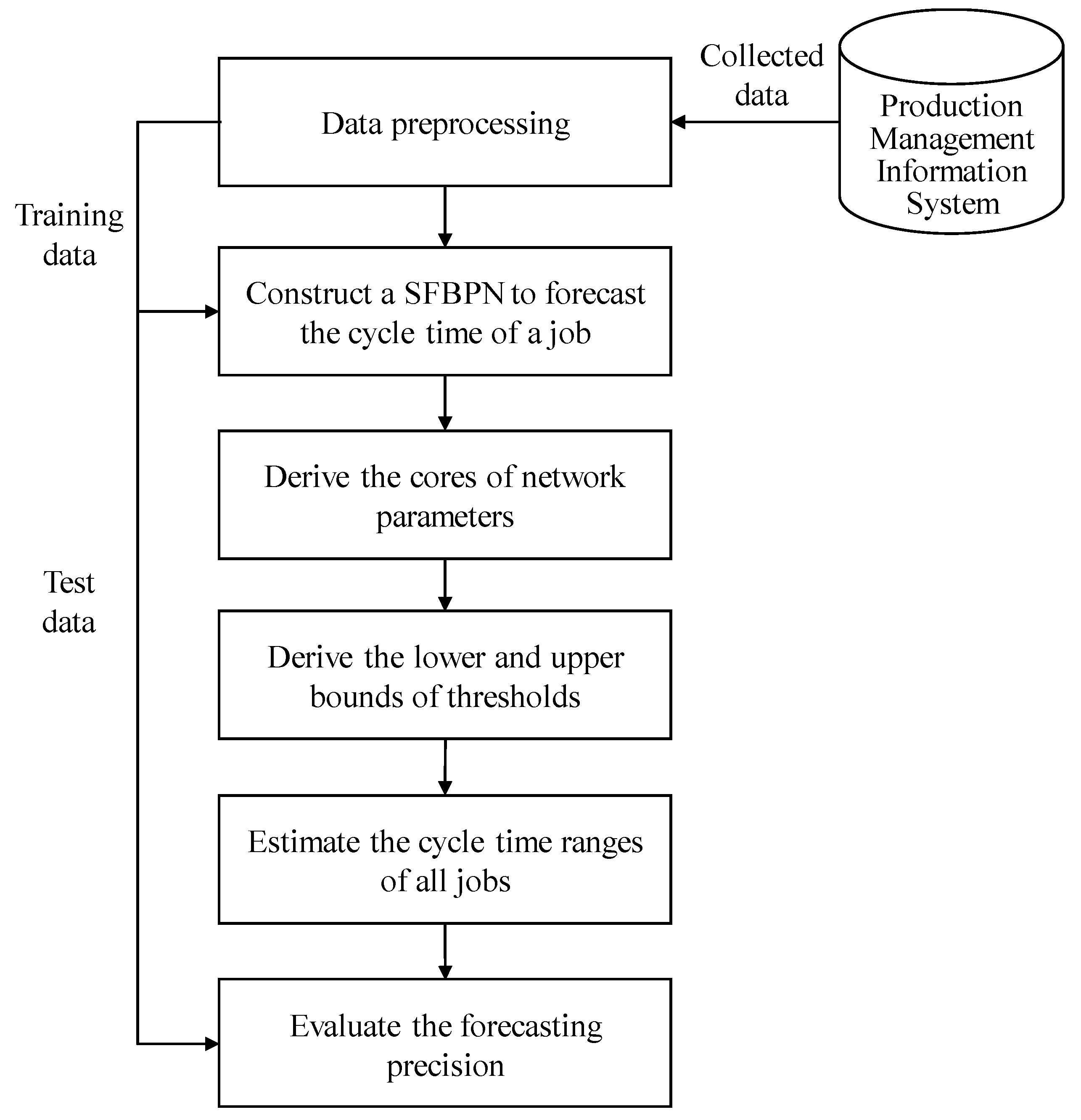
- (1)
- Preprocess the collected data: two major tasks in this step are feature selection and data normalization.
- (2)
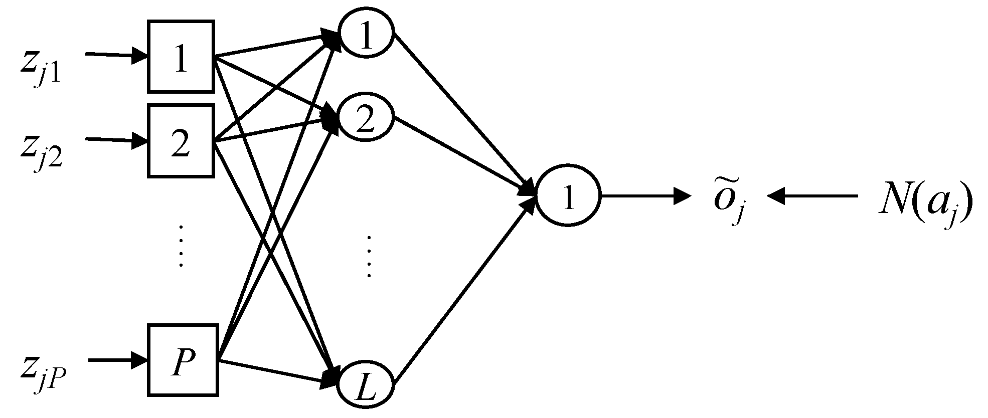
- Construct a SFBPN to forecast the cycle time of a job.
- (3)
- Train the SFBPN using an existing algorithm to derive the cores of the network parameters.
- (4)
- Apply the random search and local optimization algorithm to derive the lower and upper bounds of the thresholds.
- (5)
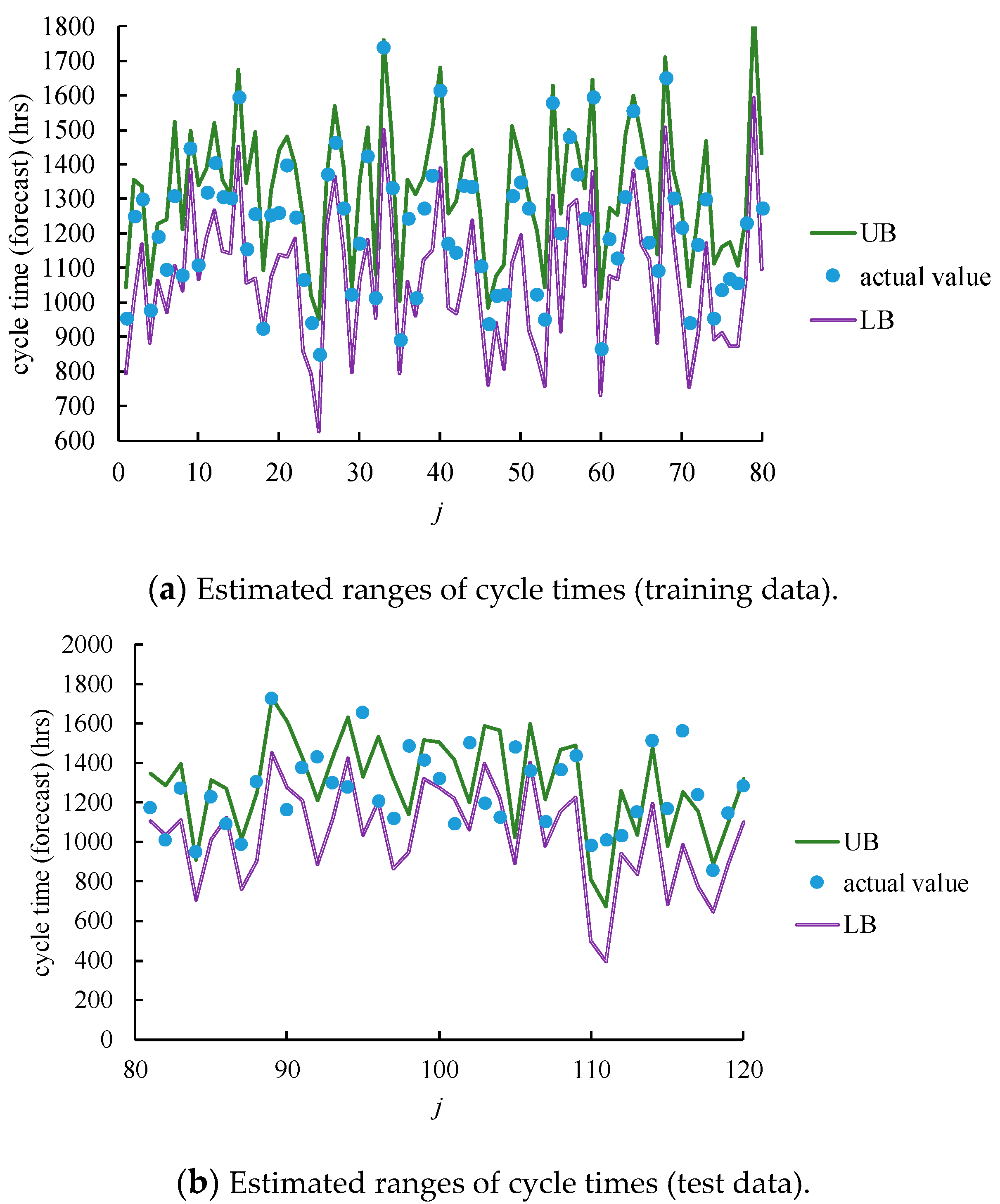
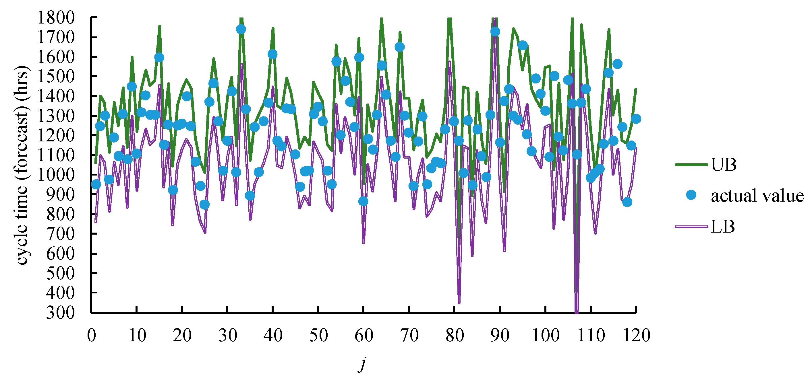
- Estimate the cycle time ranges of all of the jobs.
- (6)
- Evaluate the forecasting precision.
3.1. Data Preprocessing
3.2. Forecasting the Cycle Time of a Job Using a SFBPN
3.3. Determining the Values of Network Parameters
3.4. Fuzzifying Thresholds on Hidden-Layer Nodes
| Algorithm 1: Random search and local optimization |
| Step 1. Set t (time index) to 1. Step 2. Set (the minimum of AR so far) to a large positive value. Step 3. Set and for all l; and are random numbers within [0, v]. Step 4. Derive the values of and according to Theorem 3. Step 5. Calculate and based on the updated network parameters. Step 6. Evaluate AR. Step 7. If , set to AR and record the values of , , and . Step 8. t = t + 1. Step 9. If t > T (the number of iterations), go to Step 10; otherwise, return to Step 3. Step 10. Stop. |
4. Case Study
4.1. Background
4.2. Application of the Proposed Methodology
4.3. Comparison with Existing Methods
- (1)
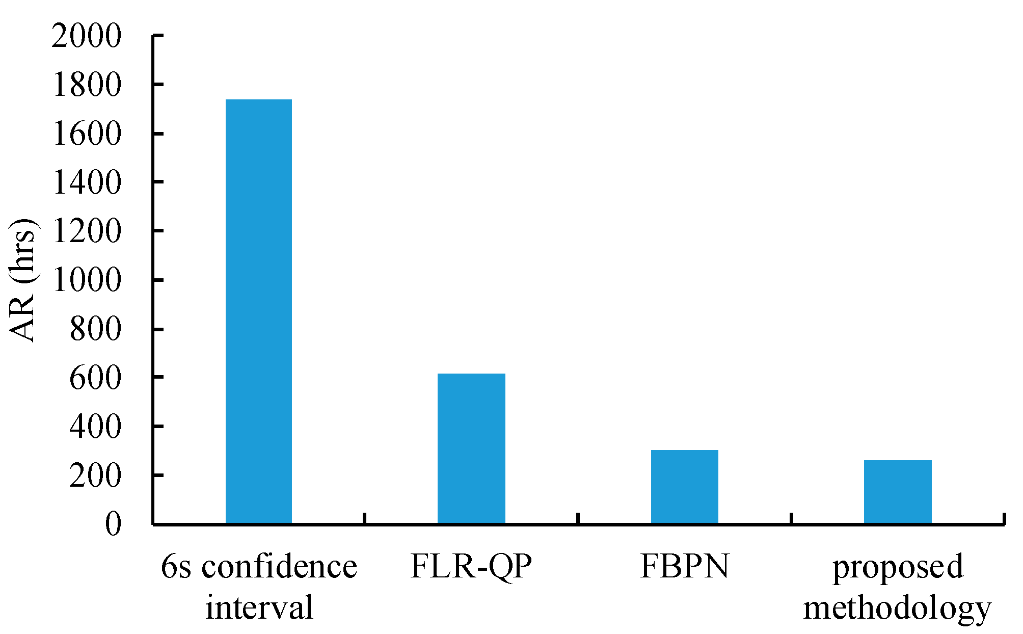
- All of the compared methods maximized the hit rate for the training data. However, the average ranges achieved using these methods differed significantly, as illustrated by Figure 7. In this regard, the proposed methodology outperformed the existing methods by establishing the narrowest range for the cycle time.
- (2)
- It is questionable whether the advantage of the SFBPN approach over the existing methods is significant. To investigate this, the following hypotheses were tested:
- (3)
- For the test data, none of these methods optimized the hit rate and the average range simultaneously. Hit rate was usually enhanced at the expense of wide ranges of fuzzy cycle time forecasts. For this sake, CFI might be a better measure for forecasting precision. In this regard, the proposed methodology surpassed the existing methods through reducing the CFI by up to 65%, as shown in Figure 8.
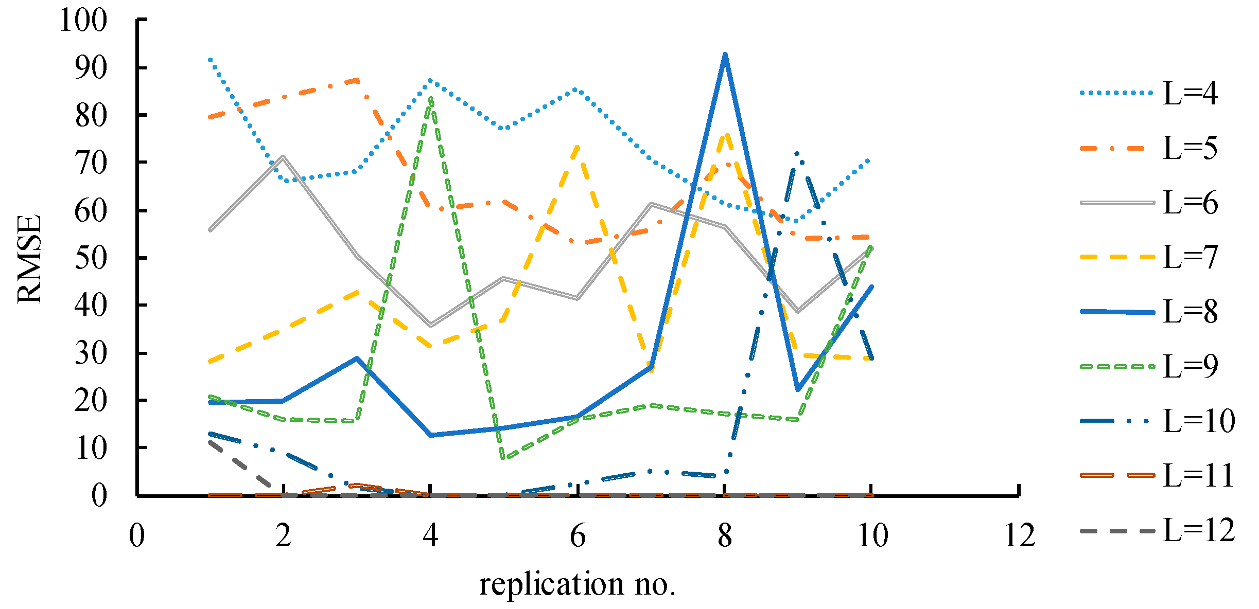
- (4)
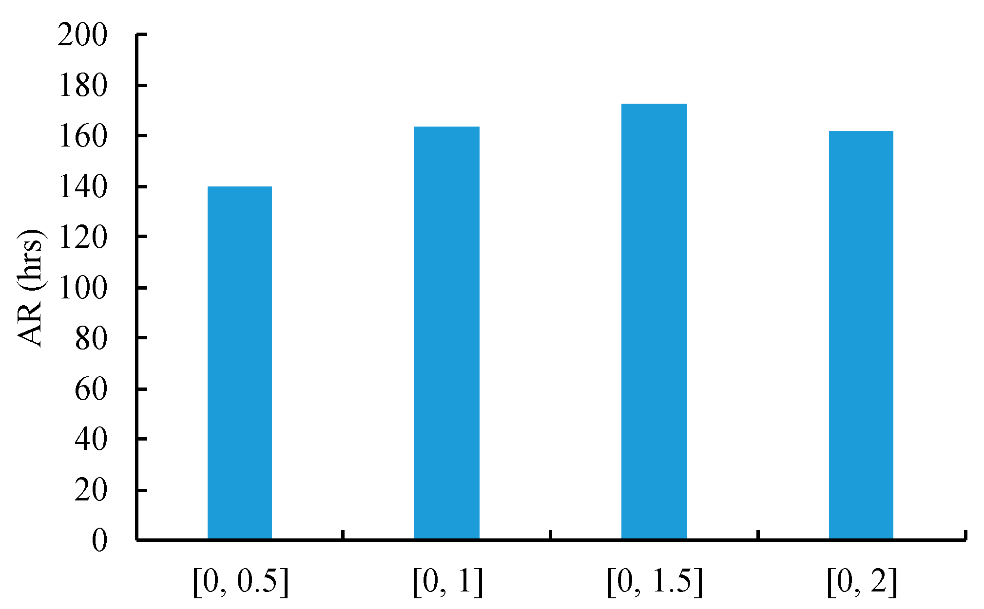
- In the random search and local optimization algorithm, it is interesting to know whether the ranges of random numbers affected the forecasting performance of the proposed methodology. To investigate this issue, various ranges of and were tried so as to observe changes in the forecasting precision. The results are summarized in Figure 9. Obviously, with a wider range, it became more difficult to find the optimal solution, which led to a poorer forecasting precision.
5. Conclusions and Future Research Directions
- (1)
- For training data (i.e., learned examples), all of the compared methods were able to include the actual values in the corresponding fuzzy cycle time forecasts or cycle time confidence intervals. However, only the proposed methodology could minimize the average ranges of the fuzzy cycle time forecasts.
- (2)
- For the test data (i.e., unlearned examples), CFI was a better measure for the forecasting precision. In this regard, the advantage of the proposed methodology over existing methods was up to 65%.
- (1)
- Although the random search and local optimization algorithm is likely to find a promising solution within a short time, it cannot guarantee the global optimality of the solution.
- (2)
- The case used to illustrate the proposed methodology is relatively small. A larger case needs to be analyzed to further elaborate the effectiveness of the proposed methodology.
Author Contributions
Funding
Institutional Review Board Statement
Informed Consent Statement
Data Availability Statement
Acknowledgments
Conflicts of Interest
References
- Baykasoğlu, A.; Göçken, M.; Unutmaz, Z.D. New approaches to due date assignment in job shops. Eur. J. Oper. Res. 2008, 187, 31–45. [Google Scholar] [CrossRef]
- Öztürk, A.; Kayalıgil, S.; Özdemirel, N.E. Manufacturing lead time estimation using data mining. Eur. J. Oper. Res. 2006, 173, 683–700. [Google Scholar] [CrossRef]
- Chang, P.C.; Liao, T.W. Combining SOM and fuzzy rule base for flow time prediction in semiconductor manufacturing factory. Appl. Soft Comput. 2006, 6, 198–206. [Google Scholar] [CrossRef]
- Chen, T. An efficient and effective fuzzy collaborative intelligence approach for cycle time estimation in wafer fabrication. Int. J. Intell. Syst. 2015, 30, 620–650. [Google Scholar] [CrossRef]
- Vinod, V.; Sridharan, R. Simulation modeling and analysis of due-date assignment methods and scheduling decision rules in a dynamic job shop production system. Int. J. Prod. Econ. 2011, 129, 127–146. [Google Scholar] [CrossRef]
- Shabtay, D. Scheduling and due date assignment to minimize earliness, tardiness, holding, due date assignment and batch delivery costs. Int. J. Prod. Econ. 2010, 123, 235–242. [Google Scholar] [CrossRef]
- Yin, Y.; Cheng, T.C.E.; Xu, D.; Wu, C.C. Common due date assignment and scheduling with a rate-modifying activity to minimize the due date, earliness, tardiness, holding, and batch delivery cost. Comput. Ind. Eng. 2012, 63, 223–234. [Google Scholar] [CrossRef]
- Tirkel, I. The effectiveness of variability reduction in decreasing wafer fabrication cycle time. In Proceedings of the 2013 Winter Simulations Conference, Washington, DC, USA, 8–11 December 2013; pp. 3796–3805. [Google Scholar]
- Asadzadeh, S.M.; Azadeh, A.; Ziaeifar, A. A neuro-fuzzy-regression algorithm for improved prediction of manufacturing lead time with machine breakdowns. Concurr. Eng. 2011, 19, 269–281. [Google Scholar] [CrossRef]
- Seidel, G.; Lee, C.F.; Tang, A.Y.; Low, S.L.; Gan, B.P.; Scholl, W. Challenges associated with realization of lot level fab out forecast in a giga wafer fabrication plant. In Proceedings of the 2020 Winter Simulation Conference, Orlando, FL, USA, 14–18 December 2020; pp. 1777–1788. [Google Scholar]
- Azadeh, A.; Ziaeifar, A.; Pichka, K.; Asadzadeh, S.M. An intelligent algorithm for optimum forecasting of manufacturing lead times in fuzzy and crisp environments. Int. J. Logist. Manag. 2013, 16, 186–210. [Google Scholar] [CrossRef]
- Malik, A.I.; Sarkar, B. Coordinating supply-chain management under stochastic fuzzy environment and lead-time reduction. Mathematics 2019, 7, 480. [Google Scholar] [CrossRef] [Green Version]
- Chen, T.; Wang, Y.C. Incorporating the FCM–BPN approach with nonlinear programming for internal due date assignment in a wafer fabrication plant. Robot. Comput. Integr. Manuf. 2010, 26, 83–91. [Google Scholar] [CrossRef]
- Wang, J.; Zhang, J. Big data analytics for forecasting cycle time in semiconductor wafer fabrication system. Int. J. Prod. Res. 2016, 54, 7231–7244. [Google Scholar] [CrossRef]
- Tan, X.; Xing, L.; Cai, Z.; Wang, G. Analysis of production cycle-time distribution with a big-data approach. J. Intell. Manuf. 2020, 31, 1889–1897. [Google Scholar] [CrossRef]
- Chen, T.; Wu, H.C. A new cloud computing method for establishing asymmetric cycle time intervals in a wafer fabrication factory. J. Intell. Manuf. 2017, 28, 1095–1107. [Google Scholar] [CrossRef] [Green Version]
- Chen, T.C.; Lin, Y.C. A collaborative fuzzy-neural approach for internal due date assignment in a wafer fabrication plant. Int. J. Innov. Comput. Inf. Control. 2011, 7, 5193–5210. [Google Scholar]
- Hsieh, L.Y.; Chang, K.H.; Chien, C.F. Efficient development of cycle time response surfaces using progressive simulation metamodeling. Int. J. Prod. Res. 2014, 52, 3097–3109. [Google Scholar] [CrossRef]
- Chang, P.C.; Wang, Y.W.; Liu, C.H. Combining SOM and GA-CBR for flow time prediction in semiconductor manufacturing factory. In Proceedings of the International Conference on Rough Sets and Current Trends in Computing, Kobe, Japan, 6–8 November 2006; pp. 767–775. [Google Scholar]
- Chen, T. Asymmetric cycle time bounding in semiconductor manufacturing: An efficient and effective back-propagation-network-based method. Oper. Res. 2016, 16, 445–468. [Google Scholar] [CrossRef]
- Wang, J.; Zhang, J.; Wang, X. Bilateral LSTM: A two-dimensional long short-term memory model with multiply memory units for short-term cycle time forecasting in re-entrant manufacturing systems. IEEE Trans. Industr. Inform. 2017, 14, 748–758. [Google Scholar] [CrossRef]
- Goodfellow, I.; Bengio, Y.; Courville, A.; Bengio, Y. Deep Learning; MIT Press: Cambridge, MA, USA, 2016. [Google Scholar]
- Montavon, G.; Samek, W.; Müller, K.R. Methods for interpreting and understanding deep neural networks. Digit Signal Process. 2018, 73, 1–15. [Google Scholar] [CrossRef]
- Wang, J.; Zhang, J.; Wang, X. A data driven cycle time prediction with feature selection in a semiconductor wafer fabrication system. IEEE Trans. Semicond. Manuf. 2018, 31, 173–182. [Google Scholar] [CrossRef]
- Kuo, P.H.; Huang, C.J. A high precision artificial neural networks model for short-term energy load forecasting. Energies 2018, 11, 213. [Google Scholar] [CrossRef] [Green Version]
- Valles, A.; Sanchez, J.; Noriega, S.; Nuñez, B.G. Implementation of Six Sigma in a manufacturing process: A case study. Int. J. Ind. Eng. 2009, 16, 171–181. [Google Scholar]
- Gani, A.N.; Assarudeen, S.M. A new operation on triangular fuzzy number for solving fuzzy linear programming problem. Appl. Math. Sci. 2012, 6, 525–532. [Google Scholar]
- Wang, J.; Ding, D.; Liu, O.; Li, M. A synthetic method for knowledge management performance evaluation based on triangular fuzzy number and group support systems. Appl. Soft Comput. 2016, 39, 11–20. [Google Scholar] [CrossRef]
- Wu, C.L.; Chau, K.W.; Fan, C. Prediction of rainfall time series using modular artificial neural networks coupled with data-preprocessing techniques. J. Hydrol. 2010, 389, 146–167. [Google Scholar] [CrossRef] [Green Version]
- Chang, P.-C.; Hsieh, J.-C. A neural networks approach for due-date assignment in a wafer fabrication factory. Eur. J. Ind. Eng. 2003, 10, 55–61. [Google Scholar]
- Martino, J.P. A review of selected recent advances in technological forecasting. Technol. Forecast. Soc. Chang. 2003, 70, 719–733. [Google Scholar] [CrossRef]
- Tirkel, I. Forecasting flow time in semiconductor manufacturing using knowledge discovery in databases. Int. J. Prod. Res. 2013, 51, 5536–5548. [Google Scholar] [CrossRef]
- Chiu, C.; Chang, P.C.; Chiu, N.H. A case-based expert support system for due-date assignment in a wafer fabrication factory. J. Intell. Manuf. 2003, 14, 287–296. [Google Scholar] [CrossRef]
- Chan, K.Y.; Kwong, C.K.; Dillon, T.S.; Tsim, Y.C. Reducing overfitting in manufacturing process modeling using a backward elimination based genetic programming. Appl. Soft Comput. 2011, 11, 1648–1656. [Google Scholar] [CrossRef]
- Chang, P.C.; Wang, Y.W.; Ting, C.J. A fuzzy neural network for the flow time estimation in a semiconductor manufacturing factory. Int. J. Prod. Res. 2008, 46, 1017–1029. [Google Scholar] [CrossRef]
- Wang, J.; Yang, J.; Zhang, J.; Wang, X.; Zhang, W. Big data driven cycle time parallel prediction for production planning in wafer manufacturing. Enterp. Inf. Syst. 2018, 12, 714–732. [Google Scholar] [CrossRef]
- Wang, J.; Zheng, P.; Zhang, J. Big data analytics for cycle time related feature selection in the semiconductor wafer fabrication system. Comput. Ind. Eng. 2020, 143, 106362. [Google Scholar] [CrossRef]
- Hanss, M. Applied Fuzzy Arithmetic; Springer: Berlin/Heidelberg, Germany, 2005. [Google Scholar]
- Yu, W.; Li, X. Fuzzy identification using fuzzy neural networks with stable learning algorithms. IEEE Trans. Fuzzy Syst. 2004, 12, 411–420. [Google Scholar] [CrossRef]
- Bonnans, J.F.; Gilbert, J.C.; Lemaréchal, C.; Sagastizábal, C.A. Numerical Optimization: Theoretical and Practical Aspects; Springer Science & Business Media: Berlin, Germany, 2006. [Google Scholar]
- Lapedus, M. Battling Fab Cycle Times. Available online: https://semiengineering.com/battling-fab-cycle-times/ (accessed on 16 February 2017).
- Hung, Y.F.; Chang, C.B. Dispatching rules using flow time predictions for semiconductor wafer fabrications. J. Chin. Inst. Ind Eng. 2002, 19, 67–75. [Google Scholar] [CrossRef]
- Donoso, S.; Marin, N.; Vila, M.A. Quadratic programming models for fuzzy regression. In Proceedings of the International Conference on Mathematical and Statistical Modeling in Honor of Enrique Castillo, Ciudad Real, Spain, 28–30 June 2006. [Google Scholar]
- Nauck, D.; Kruse, R. A fuzzy neural network learning fuzzy control rules and membership functions by fuzzy error backpropagation. In Proceedings of the IEEE International Conference on Neural Networks, San Francisco, CA, USA, 28 March–1 April 1993; pp. 1022–1027. [Google Scholar]
- Ishibuchi, H.; Kwon, K.; Tanaka, H. A learning algorithm of fuzzy neural networks with triangular fuzzy weights. Fuzzy Sets Syst. 1995, 71, 277–293. [Google Scholar] [CrossRef]
- He, W.; Dong, Y. Adaptive fuzzy neural network control for a constrained robot using impedance learning. IEEE Trans. Neural Netw. Learn. Syst. 2017, 29, 1174–1186. [Google Scholar] [CrossRef]
- Pamucar, D.; Ecer, F.; Deveci, M. Assessment of alternative fuel vehicles for sustainable road transportation of United States using integrated fuzzy FUCOM and neutrosophic fuzzy MARCOS methodology. Sci. Total Environ. 2021, 788, 147763. [Google Scholar] [CrossRef] [PubMed]
- Deveci, M.; Pamucar, D.; Gokasar, I. Fuzzy Power Heronian function based CoCoSo method for the advantage prioritization of autonomous vehicles in real-time traffic management. Sustain. Cities Soc. 2021, 69, 102846. [Google Scholar] [CrossRef]


| Method | Type of Cycle Time Forecasts | Fuzzified Parameters | Optimization Method | Precision |
|---|---|---|---|---|
| Wang and Zhang [14] | Crisp | No | Optimized feature selection | Low |
| Chen and Wu [16] | Fuzzy | Threshold on the node of the output layer | Equations based on the linear function of the output | High |
| Wang et al. [21] | Crisp | No | Deep learning | Low |
| Wang et al. [24] | Crisp | No | Optimized feature selection | Low−moderate |
| The proposed methodology | Fuzzy | Thresholds on nodes of hidden and output layers | Random search and local optimization algorithm | Very high |
| Variable | Definition |
|---|---|
| job size (pieces) | |
| fab work-in-process (WIP; jobs) | |
| queue length before the bottleneck (jobs) | |
| queue length on the processing route (jobs) | |
| average waiting time of recently completed jobs (h) | |
| fab utilization |
| Data Part | AR (h) | HR | CFI (h) |
|---|---|---|---|
| Training | 260 | 100% | 260 |
| Test | 261 | 43% | 613 |
| Data Part | AR (h) | HR | CFI (h) |
|---|---|---|---|
| Training | 1736 | 100% | 1736 |
| Test | 1736 | 100% | 1736 |
| Data Part | AR (h) | HR | CFI (h) |
|---|---|---|---|
| Training | 617 | 100% | 617 |
| Test | 616 | 100% | 616 |
| Data Part | AR (h) | HR | CFI (h) |
|---|---|---|---|
| Training | 301 | 100% | 301 |
| Test | 301 | 43% | 709 |
| 6σ Confidence Interval | FLR-QP | FBPN | SFBPN | |
|---|---|---|---|---|
| Mean | 1736.5 | 616.8 | 301.1 | 260.0 |
| Variation | 6.4 × 10⁻²⁴ | 506.6 | 77.6 | 4856.5 |
| Observations | 80 | 80 | 80 | 80 |
| Pearson correlation coefficient | 0.005 | −0.091 | −0.168 | |
| Degree of freedom | 79 | 79 | 79 | |
| t statistic | 189.5 | 42.46 | 5.12 | |
| P(T ≤ t) one-tail | 4.4 × 10−107 | 1.87 × 10−56 | 1.07 × 10⁻⁶ | |
| t Critical one-tail | 1.66 | 1.66 | 1.66 | |
| P(T ≤ t) two-tail | 8.7 × 10−107 | 3.74 × 10−56 | 2.14 × 10⁻⁶ | |
| t Critical two-tail | 1.99 | 1.99 | 1.99 |
Publisher’s Note: MDPI stays neutral with regard to jurisdictional claims in published maps and institutional affiliations. |
© 2021 by the authors. Licensee MDPI, Basel, Switzerland. This article is an open access article distributed under the terms and conditions of the Creative Commons Attribution (CC BY) license (https://creativecommons.org/licenses/by/4.0/).
Share and Cite
Wang, Y.-C.; Tsai, H.-R.; Chen, T. A Selectively Fuzzified Back Propagation Network Approach for Precisely Estimating the Cycle Time Range in Wafer Fabrication. Mathematics 2021, 9, 1430. https://doi.org/10.3390/math9121430
Wang Y-C, Tsai H-R, Chen T. A Selectively Fuzzified Back Propagation Network Approach for Precisely Estimating the Cycle Time Range in Wafer Fabrication. Mathematics. 2021; 9(12):1430. https://doi.org/10.3390/math9121430
Chicago/Turabian StyleWang, Yu-Cheng, Horng-Ren Tsai, and Toly Chen. 2021. "A Selectively Fuzzified Back Propagation Network Approach for Precisely Estimating the Cycle Time Range in Wafer Fabrication" Mathematics 9, no. 12: 1430. https://doi.org/10.3390/math9121430