
Electro-Mechanical Whole-Heart Digital Twins: A Fully Coupled Multi-Physics Approach

 , , , , and
Abstract
:1. Introduction
2. Methods
2.1. Four-Chamber Heart Model
2.2. Cardiac Elasto-Mechanics
2.2.1. Contact Boundary Conditions
2.2.2. Closed-Loop Circulatory Model
2.3. Cardiac Electrical Activity
2.4. Electro-Mechanical Coupling Mechanisms
2.4.1. Cellular Electro-Mechanical Model
2.4.2. Mechano-Electric Feedback
2.5. Electro-Mechanical Coupling Algorithm
3. Patient-Specific Simulation and Evaluation
3.1. Personalizing Electro-Mechanical Whole Heart Models: Building Digital Twins
3.1.1. Cardiac Anatomy
3.1.2. Fiber Orientation
3.1.3. Passive Stress
3.1.4. Active Stress
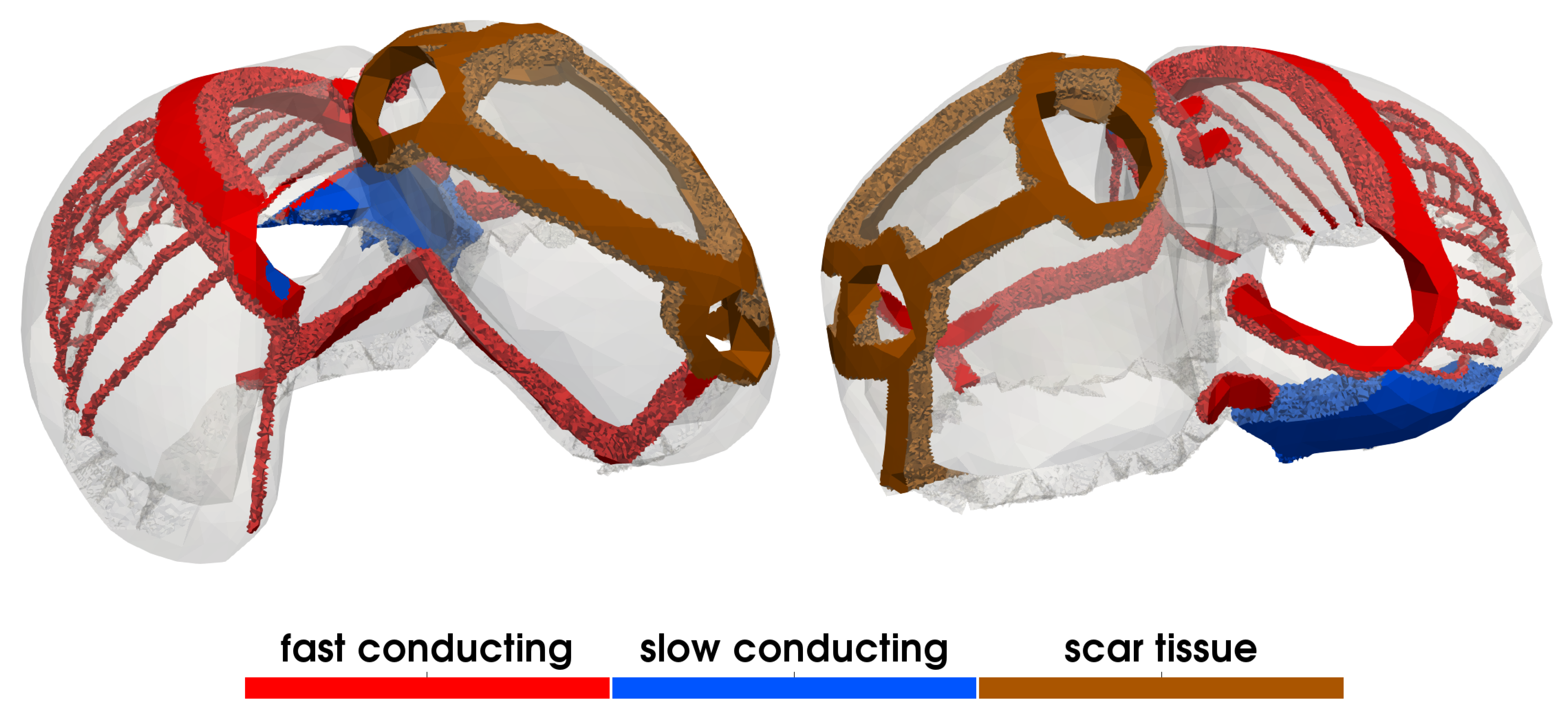
3.1.5. Electrophysiology
3.2. Experimental Setup
3.2.1. Parameterization
3.2.2. Initialization
3.2.3. Evaluation
4. Results
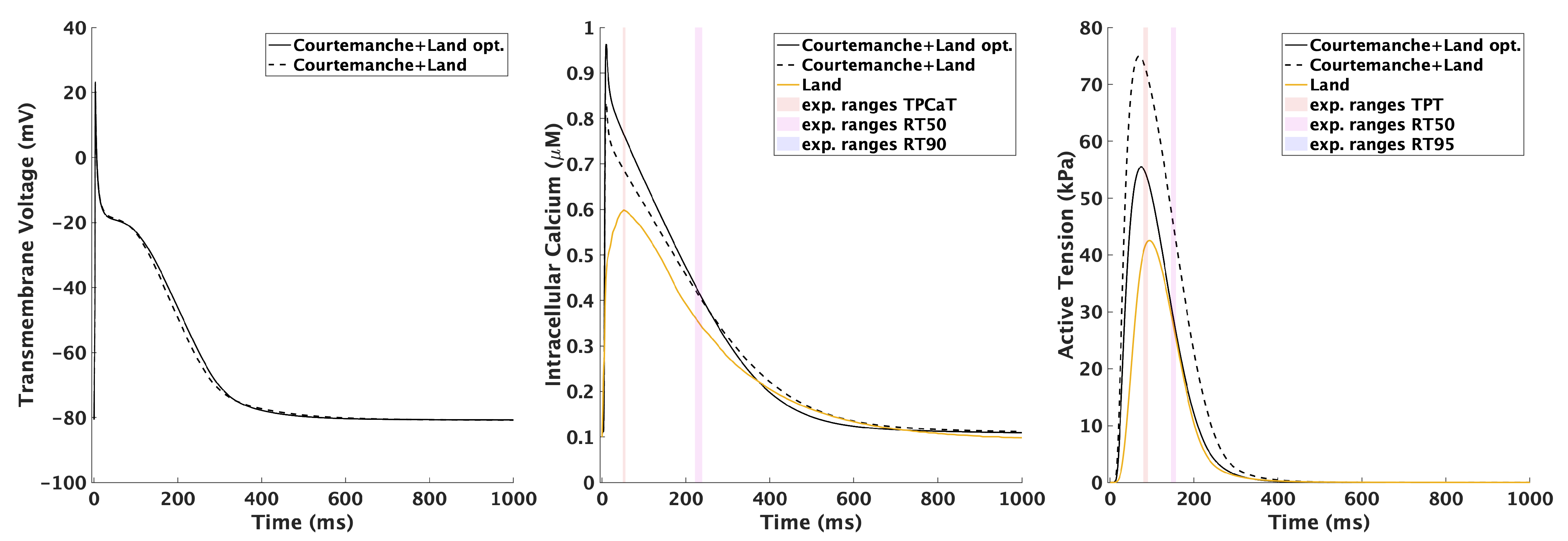
4.1. Cellular Electro-Mechanical Model
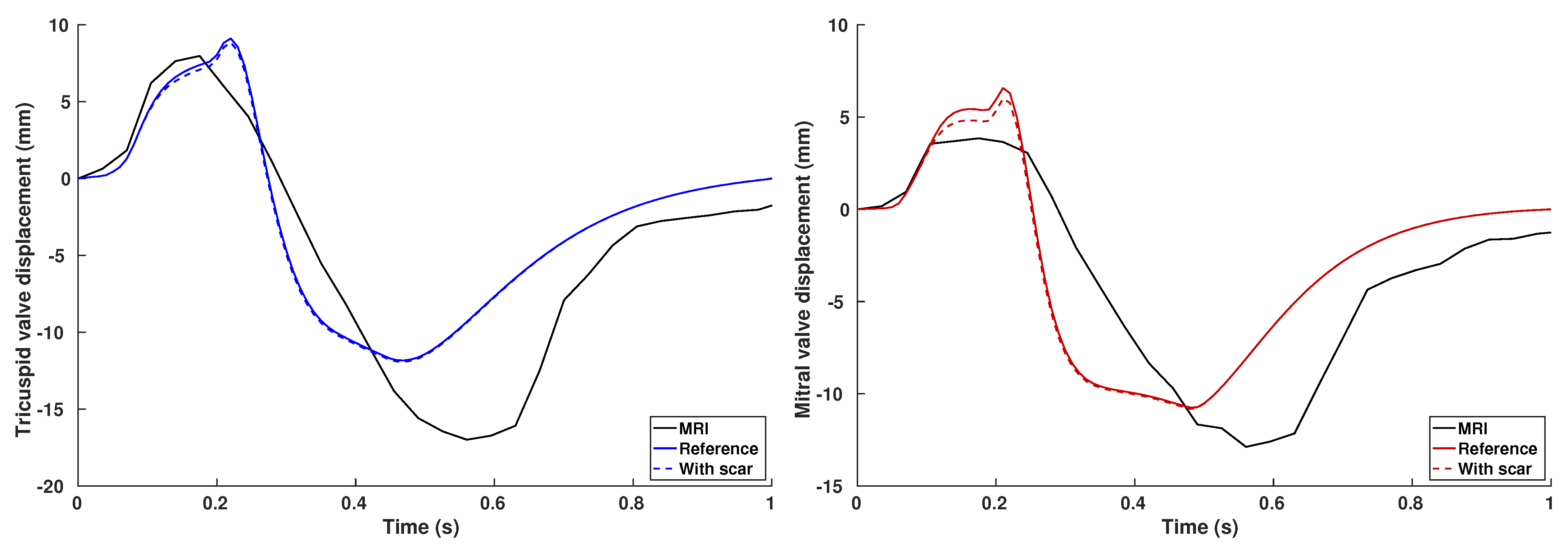
4.2. Electro-Mechanical Whole-Heart Simulation
5. Discussion
5.1. Bidirectional Coupling between the Mechanical and Electrophysiological Systems
5.2. Circulatory System
5.3. Numerical Considerations
6. Conclusions
Supplementary Materials
Author Contributions
Funding
Institutional Review Board Statement
Informed Consent Statement
Data Availability Statement
Acknowledgments
Conflicts of Interest
References
- Timmis, A.; Townsend, N.; Gale, C.P.; Torbica, A.; Lettino, M.; Petersen, S.E.; Mossialos, E.A.; Maggioni, A.P.; Kazakiewicz, D.; May, H.T.; et al. European Society of Cardiology: Cardiovascular Disease Statistics 2019. Eur. Heart J. 2019, 41, 12–85. [Google Scholar] [CrossRef] [PubMed]
- Niederer, S.A.; Lumens, J.; Trayanova, N.A. Computational models in cardiology. Nat. Rev. Cardiol. 2019, 16, 100–111. [Google Scholar] [CrossRef] [PubMed]
- Andlauer, R.; Seemann, G.; Baron, L.; Dössel, O.; Kohl, P.; Platonov, P.; Loewe, A. Influence of left atrial size on P-wave morphology: Differential effects of dilation and hypertrophy. Europace 2018, 20, iii36–iii44. [Google Scholar] [CrossRef] [PubMed]
- Arevalo, H.J.; Vadakkumpadan, F.; Guallar, E.; Jebb, A.; Malamas, P.; Wu, K.C.; Trayanova, N.A. Arrhythmia risk stratification of patients after myocardial infarction using personalized heart models. Nat. Commun. 2016, 7, 11437. [Google Scholar] [CrossRef]
- Prakosa, A.; Arevalo, H.J.; Deng, D.; Boyle, P.M.; Nikolov, P.P.; Ashikaga, H.; Blauer, J.J.E.; Ghafoori, E.; Park, C.J.; Blake, R.C.; et al. Personalized virtual-heart technology for guiding the ablation of infarct-related ventricular tachycardia. Nat. Biomed. Eng. 2018, 2, 732–740. [Google Scholar] [CrossRef]
- Loewe, A.; Poremba, E.; Oesterlein, T.; Luik, A.; Schmitt, C.; Seemann, G.; Dössel, O. Patient-Specific Identification of Atrial Flutter Vulnerability—A Computational Approach to Reveal Latent Reentry Paths. Front. Phys. 2018, 9, 1910. [Google Scholar] [CrossRef] [Green Version]
- Lehrmann, H.; Jadidi, A.S.; Minners, J.; Chen, J.; Müller-Edenborn, B.; Weber, R.; Dössel, O.; Arentz, T.; Loewe, A. Novel Electrocardiographic Criteria for Real-Time Assessment of Anterior Mitral Line Block. JACC Clin. Electrophysiol. 2018, 4, 920–932. [Google Scholar] [CrossRef]
- Corral-Acero, J.; Margara, F.; Marciniak, M.; Rodero, C.; Loncaric, F.; Feng, Y.; Gilbert, A.; Fernandes, J.F.; Bukhari, H.A.; Wajdan, A.; et al. The ‘Digital Twin’ to enable the vision of precision cardiology. Eur. Heart J. 2020, 41, 4556–4564. [Google Scholar] [CrossRef]
- Hodgkin, A.L.; Huxley, A.F. A quantitative description of membrane current and its application to conduction and excitation in nerve. J. Physiol. 1952, 117, 500–544. [Google Scholar] [CrossRef]
- Keener, J.; Sneyd, J. (Eds.) Mathematical Physology; I: Cellular Physiology; Interdisciplinary Applied Mathematics; Springer: New York, NY, USA, 2009; Volume 8/I. [Google Scholar]
- Quarteroni, A.; Lassila, T.; Rossi, S.; Ruiz-Baier, R. Integrated Heart–Coupling multiscale and multiphysics models for the simulation of the cardiac function. Comput. Methods Appl. Mech. Eng. 2017, 314, 345–407. [Google Scholar] [CrossRef] [Green Version]
- Santiago, A.; Zavala-Aké, M.; Aguado-Sierra, J.; Doste, R.; Gómez, S.; Arís, R.; Cajas, J.C.; Casoni, E.; Vázquez, M. Fully coupled fluid-electro-mechanical model of the human heart for supercomputers. Int. J. Numer. Methods Biomed. Eng. 2018, 34, e3140. [Google Scholar] [CrossRef]
- Sugiura, S.; Washio, T.; Hatano, A.; Okada, J.; Watanabe, H.; Hisada, T. Multi-scale simulations of cardiac electrophysiology and mechanics using the University of Tokyo heart simulator. Prog. Biophys. Mol. Biol. 2012, 110, 380–389. [Google Scholar] [CrossRef] [Green Version]
- Nordsletten, D.; McCormick, M.; Kilner, P.J.; Hunter, P.; Kay, D.; Smith, N.P. Fluid–solid coupling for the investigation of diastolic and systolic human left ventricular function. Int. J. Numer. Methods Biomed. Eng. 2011, 27, 1017–1039. [Google Scholar] [CrossRef]
- Arts, T.; Delhaas, T.; Bovendeerd, P.; Verbeek, X.; Prinzen, F.W. Adaptation to mechanical load determines shape and properties of heart and circulation: The CircAdapt model. Am. J. Physiol. Heart Circul. Physiol. 2005, 288, H1943–H1954. [Google Scholar] [CrossRef]
- Paeme, S.; Moorhead, K.T.; Chase, J.G.; Lambermont, B.; Kolh, P.; D’orio, V.; Pierard, L.; Moonen, M.; Lancellotti, P.; Dauby, P.C.; et al. Mathematical multi-scale model of the cardiovascular system including mitral valve dynamics. Application to ischemic mitral insufficiency. Biomed. Eng. Online 2011, 10, 86. [Google Scholar] [CrossRef] [Green Version]
- Guidoboni, G.; Sala, L.; Enayati, M.; Sacco, R.; Szopos, M.; Keller, J.M.; Popescu, M.; Despins, L.; Huxley, V.H.; Skubic, M. Cardiovascular Function and Ballistocardiogram: A Relationship Interpreted via Mathematical Modeling. IEEE Trans. Bio-Med. Eng. 2019, 66, 2906–2917. [Google Scholar] [CrossRef] [PubMed] [Green Version]
- Regazzoni, F.; Salvador, M.; Africa, P.C.; Fedele, M.; Dede’, L.; Quarteroni, A. A cardiac electromechanics model coupled with a lumped parameters model for closed-loop blood circulation. Part I: Model derivation. arXiv 2020, arXiv:2011.15040. [Google Scholar]
- Sainte-Marie, J.; Chapelle, D.; Cimrman, R.; Sorine, M. Modeling and estimation of the cardiac electromechanical activity. Comput. Struct. 2006, 84, 1743–1759. [Google Scholar] [CrossRef] [Green Version]
- Kerckhoffs, R.C.P.; Neal, M.L.; Gu, Q.; Bassingthwaighte, J.B.; Omens, J.H.; McCulloch, A.D. Coupling of a 3D Finite Element Model of Cardiac Ventricular Mechanics to Lumped Systems Models of the Systemic and Pulmonic Circulation. Ann. Biomed. Eng. 2007, 35, 1–18. [Google Scholar] [CrossRef] [PubMed] [Green Version]
- Gurev, V.; Lee, T.; Constantino, J.; Arevalo, H.; Trayanova, N.A. Models of cardiac electromechanics based on individual hearts imaging data: Image-based electromechanical models of the heart. Biomech. Model. Mechanobiol. 2011, 10, 295–306. [Google Scholar] [CrossRef] [PubMed] [Green Version]
- Gurev, V.; Pathmanathan, P.; Fattebert, J.L.; Wen, H.F.; Magerlein, J.; Gray, R.A.; Richards, D.F.; Rice, J.J. A high-resolution computational model of the deforming human heart. Biomech. Model. Mechanobiol. 2015, 14, 829–849. [Google Scholar] [CrossRef] [PubMed]
- Hirschvogel, M.; Bassilious, M.; Jagschies, L.; Wildhirt, S.M.; Gee, M.W. A monolithic 3D-0D coupled closed-loop model of the heart and the vascular system: Experiment-based parameter estimation for patient-specific cardiac mechanics. Int. J. Numer. Methods Biomed. Eng. 2017, 33, e2842. [Google Scholar] [CrossRef]
- Augustin, C.M.; Gsell, M.A.F.; Karabelas, E.; Willemen, E.; Prinzen, F.; Lumens, J.; Vigmond, E.J.; Plank, G. Validation of a 3D-0D closed-loop model of the heart and circulation—Modeling the experimental assessment of diastolic and systolic ventricular properties. arXiv 2020, arXiv:2009.08802. [Google Scholar]
- Schuler, S.; Baron, L.; Loewe, A.; Dössel, O. Developing and Coupling a Lumped Element Model of the Closed Loop Human Vascular System to a Model of Cardiac Mechanics; BMTMedPhys 2017; de Gruyter: Dresden, Germany, 2017; Volume 62, p. S69. [Google Scholar]
- Gerbi, A.; Dedè, L.; Quarteroni, A. A monolithic algorithm for the simulation of cardiac electromechanics in the human left ventricle. Math. Eng. 2019, 1, 1. [Google Scholar] [CrossRef]
- Quarteroni, A.; Dedè, L.; Manzoni, A.; Vergara, C. Mathematical Modelling of the Human Cardiovascular System: Data, Numerical Approximation, Clinical Applications; Cambridge University Press: Cambridge, UK, 2019; Volume 33. [Google Scholar]
- Garcia-Blanco, E.; Ortigosa, R.; Gil, A.J.; Bonet, J. Towards an efficient computational strategy for electro-activation in cardiac mechanics. Comput. Methods Appl. Mech. Eng. 2019, 356, 220–260. [Google Scholar] [CrossRef]
- Garcia-Blanco, E.; Ortigosa, R.; Gil, A.J.; Lee, C.H.; Bonet, J. A new computational framework for electro-activation in cardiac mechanics. Comput. Methods Appl. Mech. Eng. 2019, 348, 796–845. [Google Scholar] [CrossRef] [Green Version]
- Augustin, C.M.; Crozier, A.; Neic, A.; Prassl, A.J.; Karabelas, E.; Ferreira da Silva, T.; Fernandes, J.F.; Campos, F.; Kuehne, T.; Plank, G. Patient-specific modeling of left ventricular electromechanics as a driver for haemodynamic analysis. EP Eur. 2016, 18, iv121–iv129. [Google Scholar] [CrossRef]
- Fritz, T.; Wieners, C.; Seemann, G.; Steen, H.; Dössel, O. Simulation of the Contraction of the Ventricles in a Human Heart Model Including Atria and Pericardium. Biomech. Model. Mechanobiol. 2014, 13, 627–641. [Google Scholar] [CrossRef]
- Pfaller, M.R.; Hörmann, J.M.; Weigl, M.; Nagler, A.; Chabiniok, R.; Bertoglio, C.; Wall, W.A. The importance of the pericardium for cardiac biomechanics: From physiology to computational modeling. Biomech. Model. Mechanobiol. 2019, 18, 503–529. [Google Scholar] [CrossRef] [Green Version]
- Augustin, C.M.; Fastl, T.E.; Neic, A.; Bellini, C.; Whitaker, J.; Rajani, R.; O’Neill, M.D.; Bishop, M.J.; Plank, G.; Niederer, S.A. The impact of wall thickness and curvature on wall stress in patient-specific electromechanical models of the left atrium. Biomech. Model. Mechanobiol. 2020, 19, 1015–1034. [Google Scholar] [CrossRef] [Green Version]
- Land, S.; Niederer, S.A. Influence of atrial contraction dynamics on cardiac function. Int. J. Numer. Methods Biomed. Eng. 2018, 34, e2931. [Google Scholar] [CrossRef] [PubMed] [Green Version]
- Levrero-Florencio, F.; Margara, F.; Zacur, E.; Bueno-Orovio, A.; Wang, Z.; Santiago, A.; Aguado-Sierra, J.; Houzeaux, G.; Grau, V.; Kay, D.; et al. Sensitivity analysis of a strongly-coupled human-based electromechanical cardiac model: Effect of mechanical parameters on physiologically relevant biomarkers. Comput. Methods Appl. Mech. Eng. 2020, 361, 112762. [Google Scholar] [CrossRef]
- Margara, F.; Wang, Z.J.; Levrero-Florencio, F.; Santiago, A.; Vázquez, M.; Bueno-Orovio, A.; Rodriguez, B. In-silico human electro-mechanical ventricular modelling and simulation for drug-induced pro-arrhythmia and inotropic risk assessment. Prog. Biophys. Mol. Biol. 2021, 159, 58–74. [Google Scholar] [CrossRef]
- Prassl, A.J.; Kickinger, F.; Ahammer, H.; Grau, V.; Schneider, J.E.; Hofer, E.; Vigmond, E.J.; Trayanova, N.A.; Plank, G. Automatically generated, anatomically accurate meshes for cardiac electrophysiology problems. IEEE Trans. Bio-Med. Eng. 2009, 56, 1318–1330. [Google Scholar] [CrossRef] [PubMed] [Green Version]
- Roney, C.; Beach, M.; Mehta, A.; Sim, I.; Corrado, C.; Bendikas, R.; Alonso Solis-Lemus, J.; Razeghi, O.; Whitaker, J.; O’Neill, L.; et al. Constructing Virtual Patient Cohorts for Simulating Atrial Fibrillation Ablation. In Proceedings of the 2020 Computing in Cardiology Conference (CinC), Rimini, Italy, 13–16 September 2020; Volume 47. [Google Scholar] [CrossRef]
- Strocchi, M.; Augustin, C.M.; Gsell, M.A.F.; Karabelas, E.; Neic, A.; Gillette, K.; Razeghi, O.; Prassl, A.J.; Vigmond, E.J.; Behar, J.M.; et al. A publicly available virtual cohort of four-chamber heart meshes for cardiac electro-mechanics simulations. PLoS ONE 2020, 15, e0235145. [Google Scholar] [CrossRef] [PubMed]
- Roney, C.H.; Pashaei, A.; Meo, M.; Dubois, R.; Boyle, P.M.; Trayanova, N.A.; Cochet, H.; Niederer, S.A.; Vigmond, E.J. Universal atrial coordinates applied to visualisation, registration and construction of patient specific meshes. Med. Image Anal. 2019, 55, 65–75. [Google Scholar] [CrossRef] [PubMed]
- Bayer, J.; Prassl, A.J.; Pashaei, A.; Gomez, J.F.; Frontera, A.; Neic, A.; Plank, G.; Vigmond, E.J. Universal ventricular coordinates: A generic framework for describing position within the heart and transferring data. Med. Image Anal. 2018, 45, 83–93. [Google Scholar] [CrossRef]
- Schuler, S.; Pilia, N.; Potyagaylo, D.; Loewe, A. Cobiveco: Consistent biventricular coordinates for precise and intuitive description of position in the heart—With MATLAB implementation. arXiv 2021, arXiv:2102.02898. [Google Scholar]
- Kovacheva, E.; Baron, L.; Schuler, S.; Gerach, T.; Dössel, O.; Loewe, A. Optimization Framework to Identify Constitutive Law Parameters of the Human Heart. Curr. Direct. Biomed. Eng. 2020, 6, 95–98. [Google Scholar] [CrossRef]
- Marx, L.; Niestrawska, J.A.; Gsell, M.A.F.; Caforio, F.; Plank, G.; Augustin, C.M. Efficient identification of myocardial material parameters and the stress-free reference configuration for patient-specific human heart models. arXiv 2021, arXiv:2101.04411. [Google Scholar]
- Marx, L.; Gsell, M.A.F.; Rund, A.; Caforio, F.; Prassl, A.J.; Toth-Gayor, G.; Kuehne, T.; Augustin, C.M.; Plank, G. Personalization of electro-mechanical models of the pressure-overloaded left ventricle: Fitting of Windkessel-type afterload models. Philos. Trans. Ser. A Math. Phys. Eng. Sci. 2020, 378, 20190342. [Google Scholar] [CrossRef]
- Pezzuto, S.; Prinzen, F.W.; Potse, M.; Maffessanti, F.; Regoli, F.; Caputo, M.L.; Conte, G.; Krause, R.; Auricchio, A. Reconstruction of three-dimensional biventricular activation based on the 12-lead electrocardiogram via patient-specific modelling. EP Eur. 2020, 23, 640–647. [Google Scholar] [CrossRef]
- Potse, M.; Krause, D.; Kroon, W.; Murzilli, R.; Muzzarelli, S.; Regoli, F.; Caiani, E.; Prinzen, F.W.; Krause, R.; Auricchio, A. Patient-specific modelling of cardiac electrophysiology in heart-failure patients. Europace 2014, 16 (Suppl. 4), iv56–iv61. [Google Scholar] [CrossRef] [PubMed]
- Gillette, K.; Prassl, A.; Bayer, J.; Vigmond, E.; Neic, A.; Plank, G. Automatic Generation of Bi-Ventricular Models of Cardiac Electrophysiology for Patient Specific Personalization Using Non-Invasive Recordings. In Proceedings of the 2018 Computing in Cardiology Conference (CinC), Maastricht, The Netherlands, 23–26 September 2018; Volume 45. [Google Scholar] [CrossRef]
- Kahlmann, W.; Poremba, E.; Potyagaylo, D.; Dössel, O.; Loewe, A. Modelling of patient-specific Purkinje activation based on measured ECGs. Curr. Direct. Biomed. Eng. 2017, 3, 171–174. [Google Scholar] [CrossRef] [Green Version]
- Corrado, C.; Williams, S.; Karim, R.; Plank, G.; O’Neill, M.; Niederer, S. A work flow to build and validate patient specific left atrium electrophysiology models from catheter measurements. Med. Image Anal. 2018, 47, 153–163. [Google Scholar] [CrossRef] [PubMed]
- Grandits, T.; Pezzuto, S.; Costabal, F.S.; Perdikaris, P.; Pock, T.; Plank, G.; Krause, R. Learning atrial fiber orientations and conductivity tensors from intracardiac maps using physics-informed neural networks. arXiv 2021, arXiv:2102.10863. [Google Scholar]
- Baron, L.; Fritz, T.; Seemann, G.; Dössel, O. Sensitivity study of fiber orientation on stroke volume in the human left ventricle. In Proceedings of the Computing in Cardiology 2014, Cambridge, MA, USA, 7–10 September 2014; Volume 41, pp. 681–684. [Google Scholar]
- Kovacheva, E.; Baron, L.; Dössel, O.; Loewe, A. Electro-Mechanical Delay in the Human Heart: A Study on a Simple Geometry. In Proceedings of the Computing in Cardiology 2018, Maastricht, The Netherlands, 23–26 September 2018; Volume 45. [Google Scholar] [CrossRef]
- Müller, A.; Kovacheva, E.; Schuler, S.; Dössel, O.; Baron, L. Effects of local activation times on the tension development of human cardiomyocytes in a computational model. Curr. Direct. Biomed. Eng. 2018, 4, 247–250. [Google Scholar] [CrossRef]
- Gerach, T.; Schuler, S.; Kovacheva, E.; Dössel, O.; Loewe, A. Consequences of Using an Orthotropic Stress Tensor for Left Ventricular Systole. In Proceedings of the Computing in Cardiology Conference (CinC) 2020, Rimini, Italy, 13–16 September 2020. [Google Scholar] [CrossRef]
- Seemann, G.; Sachse, F.B.; Karl, M.; Weiss, D.L.; Heuveline, V.; Dössel, O. Framework for modular, flexible and efficient solving the cardiac bidomain equation using PETSc. Math. Ind. 2010, 15, 363–369. [Google Scholar] [CrossRef]
- Keller, D.U.J.; Kalayciyan, R.; Dössel, O.; Seemann, G. Fast creation of endocardial stimulation profiles for the realistic simulation of body surface ECGs. In Proceedings of the World Congress on Medical Physics and Biomedical Engineering, Munich, Germany, 7–12 September 2009; Volume 25/4, pp. 145–148. [Google Scholar]
- Wachter, A.; Loewe, A.; Krueger, M.W.; Dössel, O.; Seemann, G. Mesh structure-independent modeling of patient-specific atrial fiber orientation. Curr. Direct. Biomed. Eng. 2015, 1, 409–412. [Google Scholar] [CrossRef] [Green Version]
- Loewe, A. Modeling Human Atrial Patho-Electrophysiology from Ion Channels to ECG: Substrates, Pharmacology, Vulnerability, and P-Waves. Ph.D. Thesis, Karlsruhe Institute of Technology, Karlsruhe, Germany, 2016. [Google Scholar] [CrossRef]
- Gerach, T.; Weiß, D.; Dössel, O.; Loewe, A. Observation Guided Systematic Reduction of a Detailed Human Ventricular Cell Model. In Proceedings of the 2019 Computing in Cardiology (CinC), Singapore, 8–11 September 2019. [Google Scholar]
- Strocchi, M.; Gsell, M.A.; Augustin, C.M.; Razeghi, O.; Roney, C.H.; Prassl, A.J.; Vigmond, E.J.; Behar, J.M.; Gould, J.S.; Rinaldi, C.A.; et al. Simulating Ventricular Systolic Motion in a Four-chamber Heart Model with Spatially Varying Robin Boundary Conditions to Model the Effect of the Pericardium. J. Biomech. 2020, 101, 109645. [Google Scholar] [CrossRef]
- Coman, C.D. Continuum Mechanics and Linear Elasticity; Springer: Dordrecht, The Netherlands, 2020. [Google Scholar] [CrossRef]
- Ciarlet, P.G. (Ed.) Mathematical Elasticity; Volume I. Three-Dimensional Elasticity; Studies in Mathematics and Its Applications; North-Holland: Amsterdam, The Netherlands, 1988; Volume 20. [Google Scholar]
- Guccione, J.M.; McCulloch, A.D.; Waldman, L.K. Passive material properties of intact ventricular myocardium determined from a cylindrical model. J. Biomech. Eng. 1991, 113, 42–55. [Google Scholar] [CrossRef]
- Jafari, A.; Pszczolkowski, E.; Krishnamurthy, A. A framework for biomechanics simulations using four-chamber cardiac models. J. Biomech. 2019, 91, 92–101. [Google Scholar] [CrossRef] [PubMed]
- Milišić, V.; Quarteroni, A. Analysis of lumped parameter models for blood flow simulations and their relation with 1D models. ESAIM Math. Model. Numer. Anal. 2004, 38, 613–632. [Google Scholar] [CrossRef]
- Broyden, C.G. A class of methods for solving nonlinear simultaneous equations. Math. Comput. 1965, 19, 577–593. [Google Scholar] [CrossRef]
- Courtemanche, M.; Ramirez, R.J.; Nattel, S. Ionic mechanisms underlying human atrial action potential properties: Insights from a mathematical model. Am. J. Physiol.Heart Circul. Physiol. 1998, 275, H301–H321. [Google Scholar] [CrossRef] [PubMed]
- O’Hara, T.; Virag, L.; Varro, A.; Rudy, Y. Simulation of the undiseased human cardiac ventricular action potential: Model Formulation and experimental validation. PLoS Comput. Biol. 2011, 7, e1002061. [Google Scholar] [CrossRef] [Green Version]
- Passini, E.; Mincholé, A.; Coppini, R.; Cerbai, E.; Rodriguez, B.; Severi, S.; Bueno-Orovio, A. Mechanisms of pro-arrhythmic abnormalities in ventricular repolarisation and anti-arrhythmic therapies in human hypertrophic cardiomyopathy. J. Mol. Cell. Cardiol. 2016, 96, 72–81. [Google Scholar] [CrossRef] [Green Version]
- Dutta, S.; Mincholé, A.; Quinn, T.A.; Rodriguez, B. Electrophysiological properties of computational human ventricular cell action potential models under acute ischemic conditions. Prog. Biophys. Mol. Biol. 2017, 129, 40–52. [Google Scholar] [CrossRef] [PubMed]
- Land, S.; Park-Holohan, S.J.; Smith, N.P.; Dos Remedios, C.G.; Kentish, J.C.; Niederer, S.A. A model of cardiac contraction based on novel measurements of tension development in human cardiomyocytes. J. Mol. Cell. Cardiol. 2017, 106, 68–83. [Google Scholar] [CrossRef] [Green Version]
- Guharay, F.; Sachs, F. Stretch-activated single ion channel currents in tissue-cultured embryonic chick skeletal muscle. J. Physiol. 1984, 352, 685–701. [Google Scholar] [CrossRef]
- Niu, W.; Sachs, F. Dynamic properties of stretch-activated K+ channels in adult rat atrial myocytes. Prog. Biophys. Mol. Biol. 2003, 82, 121–135. [Google Scholar] [CrossRef]
- Zeng, T.; Bett, G.C.; Sachs, F. Stretch-activated whole cell currents in adult rat cardiac myocytes. Am. J. Physiol. Heart Circul. Physiol. 2000, 278, H548–H557. [Google Scholar] [CrossRef] [Green Version]
- Zhang, Y.H.; Youm, J.B.; Sung, H.K.; Lee, S.H.; Ryu, S.Y.; Ho, W.K.; Earm, Y.E. Stretch-activated and background non-selective cation channels in rat atrial myocytes. J. Physiol. 2000, 523 Pt 3, 607–619. [Google Scholar] [CrossRef] [PubMed]
- Pueyo, E.; Orini, M.; Rodríguez, J.F.; Taggart, P. Interactive effect of beta-adrenergic stimulation and mechanical stretch on low-frequency oscillations of ventricular action potential duration in humans. J. Mol. Cell. Cardiol. 2016, 97, 93–105. [Google Scholar] [CrossRef] [Green Version]
- Tavi, P.; Han, C.; Weckström, M. Mechanisms of stretch-induced changes in [Ca2+]i in rat atrial myocytes: Role of increased troponin C affinity and stretch-activated ion channels. Circul. Res. 1998, 83, 1165–1177. [Google Scholar] [CrossRef] [PubMed] [Green Version]
- Kohl, P.; Sachs, F. Mechanoelectric feedback in cardiac cells. Philos. Trans. R. Soc. Lond. Ser. A 2001, 359, 1173–1185. [Google Scholar] [CrossRef]
- Sundnes, J.; Lines, G.T.; Tveito, A. An operator splitting method for solving the bidomain equations coupled to a volume conductor model for the torso. Math. Biosci. 2005, 194, 233–248. [Google Scholar] [CrossRef]
- Crozier, A.; Augustin, C.M.; Neic, A.; Prassl, A.J.; Holler, M.; Fastl, T.E.; Hennemuth, A.; Bredies, K.; Kuehne, T.; Bishop, M.J.; et al. Image-Based Personalization of Cardiac Anatomy for Coupled Electromechanical Modeling. Ann. Biomed. Eng. 2016, 44, 58–70. [Google Scholar] [CrossRef] [PubMed] [Green Version]
- Trayanova, N.A.; Doshi, A.N.; Prakosa, A. How personalized heart modeling can help treatment of lethal arrhythmias: A focus on ventricular tachycardia ablation strategies in post-infarction patients. Wiley Interdiscip. Rev. Syst. Biol. Med. 2020, 12, e1477. [Google Scholar] [CrossRef]
- Neic, A.; Gsell, M.A.; Karabelas, E.; Prassl, A.J.; Plank, G. Automating image-based mesh generation and manipulation tasks in cardiac modeling workflows using Meshtool. SoftwareX 2020, 11, 100454. [Google Scholar] [CrossRef]
- Fedele, M.; Quarteroni, A. Polygonal surface processing and mesh generation tools for the numerical simulation of the cardiac function. Int. J. Numer. Methods Biomed. Eng. 2021, 37, e3435. [Google Scholar] [CrossRef]
- Cerqueira, M.D. American Heart Association Writing Group on Myocardial Segmentation and Registration for Cardiac Imaging: Standardized myocardial segmentation and nomenclature for tomographic imaging of the heart: A statement for healthcare professionals from the Cardiac Imaging Committee of the Council on Clinical Cardiology of the American Heart Association. Circulation 2002, 105, 539–542. [Google Scholar]
- Geerts, L.; Bovendeerd, P.; Nicolay, K.; Arts, T. Characterization of the normal cardiac myofiber field in goat measured with MR-diffusion tensor imaging. Am. J. Physiol. Heart Circ. Physiol. 2002, 283, 139. [Google Scholar] [CrossRef] [PubMed] [Green Version]
- Bayer, J.D.; Blake, R.C.; Plank, G.; Trayanova, N.A. A novel rule-based algorithm for assigning myocardial fiber orientation to computational heart models. Ann. Biomed. Eng. 2012, 40, 2243–2254. [Google Scholar] [CrossRef] [PubMed] [Green Version]
- Doste, R.; Soto-Iglesias, D.; Bernardino, G.; Alcaine, A.; Sebastian, R.; Giffard-Roisin, S.; Sermesant, M.; Berruezo, A.; Sanchez-Quintana, D.; Camara, O. A rule-based method to model myocardial fiber orientation in cardiac biventricular geometries with outflow tracts. Int. J. Numer. Methods Biomed. Eng. 2019, 35, e3185. [Google Scholar] [CrossRef] [PubMed] [Green Version]
- Wong, J.; Kuhl, E. Generating fibre orientation maps in human heart models using Poisson interpolation. Comput. Methods Biomech. Biomed. Eng. 2014, 17, 1217–1226. [Google Scholar] [CrossRef]
- Piersanti, R.; Africa, P.C.; Fedele, M.; Vergara, C.; Dedè, L.; Corno, A.F.; Quarteroni, A. Modeling cardiac muscle fibers in ventricular and atrial electrophysiology simulations. Comput. Methods Appl. Mech. Eng. 2021, 373, 113468. [Google Scholar] [CrossRef]
- Streeter, D.D.; Spotnitz, H.M.; Patel, D.P.; J, R.J.; Sonnenblick, E.H. Fiber orientation in the canine left ventricle during diastole and systole. Circ. Res. 1969, 24, 339–347. [Google Scholar] [CrossRef] [Green Version]
- Streeter, D.D.; Bassett, D.L. An engineering analysis of myocardial fiber orientation in pig’s left ventricle in systole. Anat. Rec. 1966, 155, 503–511. [Google Scholar] [CrossRef]
- Sellier, M. An iterative method for the inverse elasto-static problem. J. Fluids Struct. 2011, 27, 1461–1470. [Google Scholar] [CrossRef]
- Genet, M.; Lee, L.C.; Nguyen, R.; Haraldsson, H.; Acevedo-Bolton, G.; Zhang, Z.; Ge, L.; Ordovas, K.; Kozerke, S.; Guccione, J.M. Distribution of normal human left ventricular myofiber stress at end diastole and end systole: A target for in silico design of heart failure treatments. J. Appl. Physiol. 2014, 117, 142–152. [Google Scholar] [CrossRef] [PubMed]
- Klotz, S.; Hay, I.; Dickstein, M.L.; Yi, G.H.; Wang, J.; Maurer, M.S.; Kass, D.A.; Burkhoff, D. Single-beat estimation of end-diastolic pressure-volume relationship: A novel method with potential for noninvasive application. Am. J. Physiol. Heart Circ. Physiol. 2006, 291, H403–H412. [Google Scholar] [CrossRef] [Green Version]
- Kallhovd, S.; Sundnes, J.; Wall, S.T. Sensitivity of stress and strain calculations to passive material parameters in cardiac mechanical models using unloaded geometries. Comput. Methods Biomech. Biomed. Eng. 2019, 22, 664–675. [Google Scholar] [CrossRef] [PubMed]
- Kotadia, I.; Whitaker, J.; Roney, C.; Niederer, S.; O’Neill, M.; Bishop, M.; Wright, M. Anisotropic Cardiac Conduction. Arrhythm. Electrophysiol. Rev. 2020, 9, 202. [Google Scholar] [CrossRef] [PubMed]
- Mendonca Costa, C.; Hoetzl, E.; Martins Rocha, B.; Prassl, A.J.; Plank, G. Automatic parameterization strategy for cardiac electrophysiology simulations. In Proceedings of the Computing in Cardiology Conference (CinC) 2013, Zaragoza, Spain, 22–25 September 2013; pp. 373–376. [Google Scholar]
- Verma, B.; Oesterlein, T.; Loewe, A.; Luik, A.; Schmitt, C.; Dössel, O. Regional conduction velocity calculation from clinical multichannel electrograms in human atria. Comput. Biol. Med. 2018, 92, 188–196. [Google Scholar] [CrossRef] [PubMed]
- Niederer, S.A.; Kerfoot, E.; Benson, A.P.; Bernabeu, M.O.; Bernus, O.; Bradley, C.; Cherry, E.M.; Clayton, R.; Fenton, F.H.; Garny, A.; et al. Verification of cardiac tissue electrophysiology simulators using an N-version benchmark. Philos. Trans. R. Soc. A 2011, 369, 4331–4351. [Google Scholar] [CrossRef] [Green Version]
- Vigmond, E.J.; Stuyvers, B.D. Modeling our understanding of the His-Purkinje system. Prog. Biophys. Mol. Biol. 2016, 120, 179–188. [Google Scholar] [CrossRef]
- Gillette, K.; Prassl, A.; Bayer, J.; Vigmond, E.; Neic, A.; Plank, G. Patient-specific Parameterization of Left-ventricular Model of Cardiac Electrophysiology using Electrocardiographic Recordings. In Proceedings of the 2017 Computing in Cardiology Conference (CinC) 2017, Rennes, France, 24–27 September 2017; Volume 44. [Google Scholar] [CrossRef]
- Grandits, T.; Gillette, K.; Neic, A.; Bayer, J.; Vigmond, E.; Pock, T.; Plank, G. An Inverse Eikonal Method for Identifying Ventricular Activation Sequences from Epicardial Activation Maps. J. Comput. Phys. 2020, 419, 109700. [Google Scholar] [CrossRef]
- Cardone-Noott, L.; Bueno-Orovio, A.; Mincholé, A.; Zemzemi, N.; Rodriguez, B. Human ventricular activation sequence and the simulation of the electrocardiographic QRS complex and its variability in healthy and intraventricular block conditions. Europace 2016, 18, iv4–iv15. [Google Scholar] [CrossRef]
- Corino, V.D.A.; Sandberg, F.; Mainardi, L.T.; Sornmo, L. An atrioventricular node model for analysis of the ventricular response during atrial fibrillation. IEEE Trans. Bio-Med. Eng. 2011, 58, 3386–3395. [Google Scholar] [CrossRef]
- Schuler, S. KIT-IBT/LDRB_Fibers. Zenodo 2021. [Google Scholar] [CrossRef]
- Harrild, D.; Henriquez, C. A computer model of normal conduction in the human atria. Circ. Res. 2000, 87, E25–E36. [Google Scholar] [CrossRef] [Green Version]
- Loewe, A.; Krueger, M.W.; Holmqvist, F.; Dössel, O.; Seemann, G.; Platonov, P.G. Influence of the earliest right atrial activation site and its proximity to interatrial connections on P-wave morphology. EP Eur. 2016, 18, iv35–iv43. [Google Scholar] [CrossRef]
- Durrer, D.; van Dam, R.T.; Freud, G.E.; Janse, M.J.; Meijler, F.L.; Arzbaecher, R.C. Total excitation of the isolated human heart. Circulation 1970, 41, 899–912. [Google Scholar] [CrossRef] [Green Version]
- Smith, B.W.; Andreassen, S.; Shaw, G.M.; Jensen, P.L.; Rees, S.E.; Chase, J.G. Simulation of cardiovascular system diseases by including the autonomic nervous system into a minimal model. Comput. Methods Programs Biomed. 2007, 86, 153–160. [Google Scholar] [CrossRef]
- Hann, C.E.; Chase, J.G.; Desaive, T.; Froissart, C.B.; Revie, J.; Stevenson, D.; Lambermont, B.; Ghuysen, A.; Kolh, P.; Shaw, G.M. Unique parameter identification for cardiac diagnosis in critical care using minimal data sets. Comput. Methods Programs Biomed. 2010, 99, 75–87. [Google Scholar] [CrossRef] [PubMed] [Green Version]
- Stergiopulos, N.; Westerhof, B.E.; Westerhof, N. Total arterial inertance as the fourth element of the windkessel model. Am. J. Physiol. 1999, 276, H81–H88. [Google Scholar] [CrossRef] [PubMed]
- Murgo, J.P.; Westerhof, N.; Giolma, J.P.; Altobelli, S.A. Aortic input impedance in normal man: Relationship to pressure wave forms. Circulation 1980, 62, 105–116. [Google Scholar] [CrossRef] [PubMed] [Green Version]
- Segers, P.; Rietzschel, E.R.; De Buyzere, M.L.; Stergiopulos, N.; Westerhof, N.; Van Bortel, L.M.; Gillebert, T.; Verdonck, P.R. Three- and four-element Windkessel models: Assessment of their fitting performance in a large cohort of healthy middle-aged individuals. Proc. Inst. Mech. Eng. Part H J. Eng. Med. 2008, 222, 417–428. [Google Scholar] [CrossRef] [PubMed]
- Bovendeerd, P.H.M.; Kroon, W.; Delhaas, T. Determinants of left ventricular shear strain. Am. J. Physiol. Heart Circ. Physiol. 2009, 297, H1058–H1068. [Google Scholar] [CrossRef]
- Arts, T.; Reesink, K.; Kroon, W.; Delhaas, T. Simulation of adaptation of blood vessel geometry to flow and pressure: Implications for arterio-venous impedance. Mech. Res. Commun. 2012, 42, 15–21. [Google Scholar] [CrossRef]
- Slife, D.M.; Latham, R.D.; Sipkema, P.; Westerhof, N. Pulmonary arterial compliance at rest and exercise in normal humans. Am. J. Physiol. 1990, 258, H1823–H1828. [Google Scholar] [CrossRef] [PubMed]
- Lankhaar, J.W.; Westerhof, N.; Faes, T.J.C.; Marques, K.M.J.; Marcus, J.T.; Postmus, P.E.; Vonk-Noordegraaf, A. Quantification of right ventricular afterload in patients with and without pulmonary hypertension. Am. J. Physiol. Heart Circ. Physiol. 2006, 291, H1731–H1737. [Google Scholar] [CrossRef] [Green Version]
- Tanaka, T.; Arakawa, M.; Suzuki, T.; Gotoh, M.; Miyamoto, H.; Hirakawa, S. Compliance of human pulmonary “venous” system estimated from pulmonary artery wedge pressure tracings–comparison with pulmonary arterial compliance. Jpn. Circ. J. 1986, 50, 127–139. [Google Scholar] [CrossRef] [Green Version]
- Murgo, J.P.; Westerhof, N. Input impedance of the pulmonary arterial system in normal man. Effects of respiration and comparison to systemic impedance. Circ. Res. 1984, 54, 666–673. [Google Scholar] [CrossRef] [PubMed] [Green Version]
- Hadinnapola, C.; Li, Q.; Su, L.; Pepke-Zaba, J.; Toshner, M. The resistance-compliance product of the pulmonary circulation varies in health and pulmonary vascular disease. Physiol. Rep. 2015, 3, e12363. [Google Scholar] [CrossRef]
- Bols, J.; Degroote, J.; Trachet, B.; Verhegghe, B.; Segers, P.; Vierendeels, J. A computational method to assess the in vivo stresses and unloaded configuration of patient-specific blood vessels. J. Comput. Appl. Math. 2013, 246, 10–17. [Google Scholar] [CrossRef]
- Heiberg, E.; Sjögren, J.; Ugander, M.; Carlsson, M.; Engblom, H.; Arheden, H. Design and validation of Segment-freely available software for cardiovascular image analysis. BMC Med. Imaging 2010, 10, 1–13. [Google Scholar] [CrossRef] [PubMed] [Green Version]
- Coppini, R.; Ferrantini, C.; Yao, L.; Fan, P.; Del Lungo, M.; Stillitano, F.; Sartiani, L.; Tosi, B.; Suffredini, S.; Tesi, C.; et al. Late sodium current inhibition reverses electromechanical dysfunction in human hypertrophic cardiomyopathy. Circulation 2013, 127, 575–584. [Google Scholar] [CrossRef]
- Pieske, B.; Sütterlin, M.; Schmidt-Schweda, S.; Minami, K.; Meyer, M.; Olschewski, M.; Holubarsch, C.; Just, H.; Hasenfuss, G. Diminished post-rest potentiation of contractile force in human dilated cardiomyopathy. Functional evidence for alterations in intracellular Ca2+ handling. J. Clin. Investig. 1996, 98, 764–776. [Google Scholar] [CrossRef]
- Mulieri, L.A.; Hasenfuss, G.; Leavitt, B.; Allen, P.D.; Alpert, N.R. Altered myocardial force-frequency relation in human heart failure. Circulation 1992, 85, 1743–1750. [Google Scholar] [CrossRef] [PubMed] [Green Version]
- Rossman, E.I.; Petre, R.E.; Chaudhary, K.W.; Piacentino, V.; Janssen, P.M.L.; Gaughan, J.P.; Houser, S.R.; Margulies, K.B. Abnormal frequency-dependent responses represent the pathophysiologic signature of contractile failure in human myocardium. J. Mol. Cell. Cardiol. 2004, 36, 33–42. [Google Scholar] [CrossRef]
- Brixius, K.; Pietsch, M.; Hoischen, S.; Müller-Ehmsen, J.; Schwinger, R.H.G. Effect of inotropic interventions on contraction and Ca2+ transients in the human heart. J. Appl. Physiol. 1997, 83, 652–660. [Google Scholar] [CrossRef] [PubMed]
- Flesch, M.; Kilter, H.; Cremers, B.; Lenz, O.; Südkamp, M.; Kuhn-Regnier, F.; Böhm, M. Acute effects of nitric oxide and cyclic GMP on human myocardial contractility. J. Pharmacol. Exp. Ther. 1997, 281, 1340–1349. [Google Scholar]
- Geuzaine, C.; Remacle, J.F. Gmsh: A 3-D finite element mesh generator with built-in pre-and post-processing facilities. Int. J. Numer. Methods Eng. 2009, 79, 1309–1331. [Google Scholar] [CrossRef]
- Whiteley, J.P.; Bishop, M.J.; Gavaghan, D.J. Soft tissue modelling of cardiac fibres for use in coupled mechano-electric simulations. Bull. Math. Biol. 2007, 69, 2199–2225. [Google Scholar] [CrossRef]
- Augustin, C.M.; Neic, A.; Liebmann, M.; Prassl, A.J.; Niederer, S.A.; Haase, G.; Plank, G. Anatomically accurate high resolution modeling of human whole heart electromechanics: A strongly scalable algebraic multigrid solver method for nonlinear deformation. J. Comput. Phys. 2016, 305, 622–646. [Google Scholar] [CrossRef] [PubMed] [Green Version]
- Sachse, F.B.; Glänzel, K.; Seemann, G. Modeling of protein interactions involved in cardiac tension development. Int. J. Bifurc. Chaos 2003, 13, 3561–3578. [Google Scholar] [CrossRef]
- Campbell, K.S. Compliance Accelerates Relaxation in Muscle by Allowing Myosin Heads to Move Relative to Actin. Biophys. J. 2016, 110, 661–668. [Google Scholar] [CrossRef] [Green Version]
- Regazzoni, F.; Quarteroni, A. An oscillation-free fully staggered algorithm for velocity-dependent active models of cardiac mechanics. Comput. Methods Appl. Mech. Eng. 2021, 373, 113506. [Google Scholar] [CrossRef]
- Land, S.; Gurev, V.; Arens, S.; Augustin, C.M.; Baron, L.; Blake, R.; Bradley, C.; Castro, S.; Crozier, A.; Favino, M.; et al. Verification of cardiac mechanics software: Benchmark problems and solutions for testing active and passive material behaviour. Proc. R. Soc. Lond. A 2015, 471, 20150641. [Google Scholar] [CrossRef] [PubMed] [Green Version]
- Woodworth, L.A.; Cansız, B.; Kaliske, M. A numerical study on the effects of spatial and temporal discretization in cardiac electrophysiology. Int. J. Numer. Methods Biomed. Eng. 2021, 37, e3443. [Google Scholar] [CrossRef] [PubMed]
- ten Tusscher, K.H.; Noble, D.; Noble, P.J.; Panfilov, A.V. A model for human ventricular tissue. Am. J. Physiol. Heart Circ. Physiol. 2004, 286, H1573–H1589. [Google Scholar] [CrossRef] [PubMed]
- Andreianov, B.; Bendahmane, M.; Quarteroni, A.; Ruiz-Baier, R. Solvability analysis and numerical approximation of linearized cardiac electromechanics. Math. Models Methods Appl. Sci. 2015, 25, 959–993. [Google Scholar] [CrossRef] [Green Version]
- Mroue, F. Cardiac Electromechanical Coupling: Modeling, Mathematical Analysis and Numerical Simulation. Ph.D. Thesis, Ecole Centrale de Nantes (ECN). Université Libanaise, Beirut, Lebanon, 2019. [Google Scholar]


| Parameter | Value | Unit | Description |
|---|---|---|---|
| S/m | conductivities in ventricular bulk tissue | ||
| S/m | conductivities in ventricular fast conducting layer | ||
| S/m | conductivities in atrial bulk tissue | ||
| S/m | conductivities in atrial fast conducting regions | ||
| S/m | conductivities in atrial slow conducting regions | ||
| S/m | conductivities in scar tissue | ||
| 140,000 | 1/m | membrane surface-to-volume ratio | |
| F/m | membrane capacitance | ||
| AV-delay | s | atrio-ventricular conduction delay | |
| BCL | 1 | s | basic cycle length (=) |
| Root Point | Extent | ||
|---|---|---|---|
| 3 mm | |||
| 3 mm | |||
| 3 mm | |||
| 3 mm | |||
| 3 mm | |||
| Parameters | |||||||
|---|---|---|---|---|---|---|---|
| Domain | Model | (Pa) | (Pa) | (kg/m) | |||
| Guccione | 1082 | ||||||
| Guccione | 1082 | ||||||
| Neo-Hooke | - | - | - | 1082 | |||
| Neo-Hooke | 3725 | - | - | - | 1082 | ||
| Neo-Hooke | - | - | - | 1082 | |||
| Neo-Hooke | - | - | - | 1082 | |||
| Parameter | Value | Unit | Description | Ref. |
|---|---|---|---|---|
| 0.006 | aortic valve resistance | [110,111] | ||
| 0.03 | systemic arterial resistance | [112,113] | ||
| 3.0 | systemic arterial compliance | [112,113,114] | ||
| 800.0 | mL | unstressed systemic arterial volume | [110] | |
| 0.6 | systemic peripheral resistance | [112,113] | ||
| 0.03 | systemic venous resistance | [115,116] | ||
| 150.0 | systemic venous compliance | [110,111,116] | ||
| 2850.0 | mL | unstressed systemic venous resistance | [110,115] | |
| 0.003 | tricuspid valve resistance | [20,111] | ||
| 0.003 | pulmonary valve resistance | [110] | ||
| 0.02 | pulmonary arterial resistance | [117,118] | ||
| 10.0 | pulmonary arterial compliance | [117,119] | ||
| 150.0 | mL | unstressed pulmonary arterial volume | [110] | |
| 0.07 | pulmonary peripheral resistance | [120,121] | ||
| 0.03 | pulmonary venous resistance | [20] | ||
| 15.0 | pulmonary venous compliance | [119] | ||
| 200.0 | mL | unstressed pulmonary venous volume | [110] | |
| 0.003 | mitral valve resistance | [20] |
| Parameter | Value | Unit | Description |
|---|---|---|---|
| 5700.0 | mL | total volume | |
| 981.1396 | mL | systemic arterial volume | |
| 303.7683 | mL | pulmonary arterial volume | |
| 349.6759 | mL | pulmonary venous volume | |
| 8.0246 | mmHg | left ventricular pressure | |
| 8.2061 | mmHg | left atrial pressure | |
| 5.8073 | mmHg | right ventricular pressure | |
| 5.8071 | mmHg | right atrial pressure |
| Calcium Transient | Active Tension | ||||||
|---|---|---|---|---|---|---|---|
| Tissue | TPCaT (ms) | RT50 (ms) | RT90 (ms) | TPT (ms) | RT50 (ms) | RT95 (ms) | Ref. |
| Ventricle | - | - | - | [124] | |||
| Ventricle | - | - | - | [125] | |||
| Ventricle | - | - | - | [126] | |||
| Ventricle | - | - | - | [127] | |||
| Ventricle | - | - | - | [127] | |||
| Atria | - | - | [128] | ||||
| Atria | - | - | - | - | [129] | ||
| Atria | - | - | - | - | [129] | ||
| Atria | Ventricle | |||
|---|---|---|---|---|
| Parameter | Original Value | Optimized | Original Value | Optimized |
| 1/ms | 1/ms | 1/ms | 0.04/ms | |
| 5 | 5 | 5 | 2.4 | |
| 0.86 µM | 1.05 µM | 0.805 µM | 1.05 µM | |
| −2.4 | −0.5 | −2.4 | −2.4 | |
Publisher’s Note: MDPI stays neutral with regard to jurisdictional claims in published maps and institutional affiliations. |
© 2021 by the authors. Licensee MDPI, Basel, Switzerland. This article is an open access article distributed under the terms and conditions of the Creative Commons Attribution (CC BY) license (https://creativecommons.org/licenses/by/4.0/).
Share and Cite
Gerach, T.; Schuler, S.; Fröhlich, J.; Lindner, L.; Kovacheva, E.; Moss, R.; Wülfers, E.M.; Seemann, G.; Wieners, C.; Loewe, A. Electro-Mechanical Whole-Heart Digital Twins: A Fully Coupled Multi-Physics Approach. Mathematics 2021, 9, 1247. https://doi.org/10.3390/math9111247
Gerach T, Schuler S, Fröhlich J, Lindner L, Kovacheva E, Moss R, Wülfers EM, Seemann G, Wieners C, Loewe A. Electro-Mechanical Whole-Heart Digital Twins: A Fully Coupled Multi-Physics Approach. Mathematics. 2021; 9(11):1247. https://doi.org/10.3390/math9111247
Chicago/Turabian StyleGerach, Tobias, Steffen Schuler, Jonathan Fröhlich, Laura Lindner, Ekaterina Kovacheva, Robin Moss, Eike Moritz Wülfers, Gunnar Seemann, Christian Wieners, and Axel Loewe. 2021. "Electro-Mechanical Whole-Heart Digital Twins: A Fully Coupled Multi-Physics Approach" Mathematics 9, no. 11: 1247. https://doi.org/10.3390/math9111247