A Novel Analysis of the Smooth Curve with Constant Width Based on a Time Delay System

Abstract

In this paper, we analyze the $C^{\infty }$ smooth curve of constant width using the characteristic equation of a time delay system. We prove that a closed convex curve must be a circle if it is still a smooth curve of constant width after taking any number of derivatives. Finally, the simulation results are presented for analyzing the influence of derivative orders on a smooth non-circular curve of constant width.

1. Introduction

The curves of constant width are a type of interesting curve that can be used to design precise mechanical structures [1]. Since Euler first proposed the concept of the curve of constant width, researches of the non-circular curve of constant width have attracted extensive attention [1,2,3,4]. In 1876, an engineer named Reuleaux constructed a curve of constant width that was based on an equilateral triangle, which is now known as the Reuleaux triangle. In 1997, Rabinowitz [5] investigated the non-circular curve of constant width and found its parametric equation, so as to plot the curve with a graphing calculator. In 2010, Paciotti [6] studied the curves of constant width and the shadows that they cast, and then used the shadows to distinguish different curves. In 2011, Xu et al. [7] used an isosceles trapezoid to construct another curve of constant width. This basic construction process can be generalized to construct curves of constant width that are based on special 2n-sided polygons with N groups parallel to the opposite sides. In 2015, Yang [8] constructed a non-circular curve of constant width using the opposite top sector, and the obtained curve of constant width included the results by Reuleaux and [7]. Additionally, Mozgawa [9] provided a generalization of the theorem characterizing ovals of constant width proved by Mellish [10]. Moreover, Resnikoff [11] investigated the curves and surfaces of constant width by means of Fourier series, with some additional results regarding general ovals. However, the main drawback of these methods is that the constructed curves of constant width are piecewise smooth. To address this issue, on the basis of the piecewise smooth curve, a $C^1$ curve of constant width with better smoothness can be constructed using the outer parallel lines [12]. In order to obtain a smoother curve of constant width, a class of $C^{\infty }$ smooth non-circular curves of constant width is constructed using the tangent polar coordinates of the plane curve based on the Minkowski support function [13]. However, in terms of these constructions, the first derivative of the parametric equation yields a curve with a self-intersection point, instead of a $C^{\infty }$ smooth curve.

Being motivated by the above analysis, it is natural to propose the following problem: whether there exists a $C^{\infty }$ smooth non-circular curve of constant width, such that its parametric equation after taking any number of derivatives still represents a smooth curve of constant width. In this paper, we aim to prove that there is no $C^{\infty }$ smooth non-circular curve of constant width in theory, so that the parametric equation after taking any number of derivatives is still a smooth curve of constant width. Moreover, the simulation results are proposed to further illustrate this hypothesis.

The remainder of this paper is structured as follows. In Section 2, the related preliminaries and a hypothesis are presented. Section 3 provides the proof of the proposed hypothesis. Simulation results are reported and discussed in Section 4. Finally, some conclusions are given in Section 5.

2. Preliminaries and a Hypothesis

Let $\Gamma$ be a smooth closed curve in the plane $R^2$, and define an arbitrary point in the region that is bounded by the curve $\Gamma$ as the origin point of the plane $R^2$. A positive oriented coordinate system is established as $XOY$. $\theta$ represents the angle between the positive direction of the $OX$ axis and the perpendicular line that corresponds to the tangent line of $\Gamma$. Moreover, $P\left(\theta \right)$ denotes the distance from the origin O to the tangent line of $\Gamma$, which is called the support function of the curve $\Gamma$.

Setting $(x,y)$ as a point on $\Gamma$, it follows from the support function $P\left(\theta \right)$ that

$$x\cos \theta +y\sin \theta -P\left(\theta \right)=0.$$

(1)

Differentiating both sides of (1) with respect to $\theta$ gives

$$-x\sin \theta +y\cos \theta -\dot{P}\left(\theta \right)=0.$$

(2)

When combining (1) with (2), the parametric equation of $\Gamma$ can be formulated by

$$\left\{\begin{array}{c}x=P\left(\theta \right)\cos \theta -\dot{P}\left(\theta \right)\sin \theta ,\hfill \\ y=P\left(\theta \right)\sin \theta +\dot{P}\left(\theta \right)\cos \theta ,\hfill \end{array}\right.\theta \in [0,2\pi ).$$

(3)

If $\Gamma$ is a smooth closed convex curve, then its support function should satisfy the following necessary and sufficient conditions.

Lemma 1

([14]). The function $P\left(\theta \right)$ of period $2\pi$ is the support function of a smooth closed convex curve, if and only if

$$P\left(\theta \right)+\ddot{P}\left(\theta \right)>0,\theta \in [0,2\pi ).$$

(4)

Now, we would like to consider an interesting curve: a smooth curve of constant width. First, we present the definition of the width of a simple closed convex curve.

Definition 1.

The width function of a closed convex curve Γ is defined as

$$D\left(\theta \right)=P\left(\theta \right)+P(\theta +\pi ).$$

(5)

If $D\left(\theta \right)=d$ is a constant, then Γ is called a curve of constant width.

The $C^{\infty }$ smooth curve of constant width is the research objective of this paper. The so-called $C^{\infty }$ smooth curve means that each component of its parametric equation is infinitely differentiable, namely, $P\left(\theta \right)$ is infinitely differentiable. At present, many researchers have proposed several methods to construct curves of constant width. However, these constructed curves of constant width either have corners, such as the Reuleaux polygon, or have better smoothness derived from outer parallel lines, but the derivative of which is not smooth again. In addition, there are also some curves of constant width that can be infinitely differentiated, whereas, after several derivatives the resulting equations no longer represent curves of constant width.

Accordingly, it is natural to propose the following hypothesis.

Hypothesis 1.

For a $C^{\infty }$ smooth curve Γ of constant width, if its parametric equation is still a smooth curve of constant width after any number of derivatives, then the curve Γ must be a circle.

3. The Proof of the Hypothesis

Assume that the width of the $C^{\infty }$ smooth curve $\Gamma$ is d, namely,

$$P\left(\theta \right)+P(\theta +\pi )=d,$$

(6)

which is equivalent to

$$P\left(\theta \right)+P(\theta -\pi )=d.$$

(7)

After differentiating both sides of (7) with respect to $\theta$, one has

$$\dot{P}\left(\theta \right)+\dot{P}(\theta -\pi )=0,$$

(8)

which stands for a neutral delay differential equation.

Setting $P\left(\theta \right)=\tilde{C}{\mathrm{e}}^{\lambda \theta }$, and then substituting it into (8) gives the following characteristic equation

$$\lambda {\mathrm{e}}^{\lambda \theta }+\lambda {\mathrm{e}}^{\lambda (\theta -\pi )}=0,$$

(9)

which yields

$$1+{\mathrm{e}}^{-\lambda \pi }=0\mathrm{or}\lambda =0.$$

(10)

When $\lambda =0$, we obtain $P\left(\theta \right)=\tilde{C}=\frac{d}{2}$. In this case, $\Gamma$ is a circle of radius $\frac{d}{2}$. When $\lambda \ne 0$, it is obvious that $\lambda$ cannot be a real number. Accordingly, when setting $\lambda =\alpha +\omega i$ and substituting it into (10), one has

$${\mathrm{e}}^{-\pi \alpha }[\cos \left(\omega \pi \right)-i\sin \left(\omega \pi \right)]=-1.$$

(11)

It follows from (11) that

$$\left\{\begin{array}{c}{\mathrm{e}}^{-\pi \alpha }\cos \left(\omega \pi \right)=-1,\hfill \\ {\mathrm{e}}^{-\pi \alpha }\sin \left(\omega \pi \right)=0,\hfill \end{array}\right.$$

(12)

which implies

$$\left\{\begin{array}{c}\sin \left(\omega \pi \right)=0,\hfill \\ \cos \left(\omega \pi \right)=-1,{\mathrm{e}}^{-\pi \alpha }=1.\hfill \end{array}\right.$$

(13)

Furthermore, we obtain

$$\alpha =0,\omega =2k+1,k\in Z.$$

(14)

Therefore, the general solution of (8) is expressed as

$$P\left(\theta \right)=C_1\cos \left(\omega \theta \right)+C_2\sin \left(\omega \theta \right)+C_3.$$

(15)

When substituting (15) into (6), one has

$$C_3=\frac{d}{2}.$$

(16)

It follows from (15) and (16) that

$$P\left(\theta \right)=C\sin (\omega \theta +\phi )+\frac{d}{2},$$

(17)

where $C=\sqrt{C_1^2+C_2^2}$ with constants $C_1,C_2$ being decided by the initial condition, $\phi$ is an angle, and its value can be derived from $sin\phi =\frac{C_1}{\sqrt{C_1^2+C_2^2}}$ or $cos\phi =\frac{C_2}{\sqrt{C_1^2+C_2^2}}$. By using Lemma 1, we see that the smooth curve $\Gamma$ is a closed convex curve, if and only if

$$\frac{d}{2}-C({\omega }^2-1)>0.$$

(18)

For simplicity, we assume that the support function is

$$P\left(\theta \right)=C\sin \left(\omega \theta \right)+\frac{d}{2}.$$

(19)

Substituting (19) into (3) gives

$$\left\{\begin{array}{c}x=[\frac{d}{2}+C\sin \left(\omega \theta \right)]\cos \theta -C\omega \cos \left(\omega \theta \right)\sin \theta ,\hfill \\ y=[\frac{d}{2}+C\sin \left(\omega \theta \right)]\sin \theta +C\omega \cos \left(\omega \theta \right)\cos \theta .\hfill \end{array}\right.$$

(20)

Equation (20) can be rewritten as

$$\left\{\begin{array}{c}x=\frac{d}{2}\cos \theta +\frac{C}{2}\left[\sin \left[\right(\omega +1\left)\theta \right]+\sin \left[\right(\omega -1\left)\theta \right]\right]-\frac{C\omega }{2}\left[\sin \left[\right(\omega +1\left)\theta \right]-\sin \left[\right(\omega -1\left)\theta \right]\right],\hfill \\ y=\frac{d}{2}\sin \theta +\frac{C}{2}\left[\cos \left[\right(\omega -1\left)\theta \right]-\cos \left[\right(\omega +1\left)\theta \right]\right]+\frac{C\omega }{2}\left[\cos \left[\right(\omega +1\left)\theta \right]+\cos \left[\right(\omega -1\left)\theta \right]\right].\hfill \end{array}\right.$$

(21)

In what follows, we would like to discuss the curves $\Gamma$ described by (21) in different values of $\omega$. From (14), we see that $\omega =2k+1,k\in Z$. Therefore, we will analyze the two cases of $\omega =1$ and $\omega >1$, respectively. When $\omega =1$, (21) becomes

$$\left\{\begin{array}{c}x=\frac{d}{2}\cos \theta ,\hfill \\ y=\frac{d}{2}\sin \theta +C,\hfill \end{array}\right.$$

(22)

which implies that the curve $\Gamma$ is a circle.

When $\omega >1$, taking the n-th derivative of (21) with respect to $\theta$ gives

$$\left\{\begin{array}{cc}{x}^{\left(n\right)}=\hfill & \frac{d}{2}\cos (\theta +\frac{1}{2}n\pi )+\frac{C}{2}\left[\sin [(\omega +1)\theta +\frac{1}{2}n\pi ]{(\omega +1)}^n+\sin [(\omega -1)\theta +\frac{1}{2}n\pi ]{(\omega -1)}^n\right]\hfill \\ \hfill & -\frac{C\omega }{2}\left[\sin [(\omega +1)\theta +\frac{1}{2}n\pi ]{(\omega +1)}^n-\sin [(\omega -1)\theta +\frac{1}{2}n\pi ]{(\omega -1)}^n\right],\hfill \\ y^{\left(n\right)}=\hfill & \frac{d}{2}\sin (\theta +\frac{1}{2}n\pi )+\frac{C}{2}\left[\cos [(\omega -1)\theta +\frac{1}{2}n\pi ]{(\omega -1)}^n-\cos [(\omega +1)\theta +\frac{1}{2}n\pi ]{(\omega +1)}^n\right]\hfill \\ \hfill & +\frac{C\omega }{2}\left[\cos [(\omega +1)\theta +\frac{1}{2}n\pi ]{(\omega +1)}^n+\cos [(\omega -1)\theta +\frac{1}{2}n\pi ]{(\omega -1)}^n\right].\hfill \end{array}\right.$$

(23)

From (23), we see that, when n is large enough, the term containing ${(\omega +1)}^n$ plays a predominant role in the parametric equation. In this case, (23) can be approximated to the following equation

$$\left\{\begin{array}{cc}{x}^{\left(n\right)}=\hfill & \frac{C}{2}(1-\omega ){(\omega +1)}^n\sin [(\omega +1)\theta +\frac{1}{2}n\pi ],\hfill \\ y^{\left(n\right)}=\hfill & \frac{C}{2}(\omega -1){(\omega +1)}^n\cos [(\omega +1)\theta +\frac{1}{2}n\pi ],\hfill \end{array}\right.\theta \in [0,2\pi ).$$

(24)

System (24) comprises a circle of radius $|\frac{C}{2}(1-\omega ){(\omega +1)}^n|$, and this circle goes around $(\omega +1)$ times when $\theta \in [0,2\pi )$. As a result, when n is large enough, the trajectory of system (24) is no longer a simple closed curve.

From the above analysis, we see that $\Gamma$ is still a $C^{\infty }$ smooth curve of constant width after taking any times of derivatives, if and only if $\omega =1$. This proves the hypothesis.

Remark 1.

Although different non-circular smooth curves of constant width have been constructed in the literature, the obtained curves after taking any number of derivatives have not been further studied. From the proof procedure shown above, it can be seen that a non-circular curve of constant width is no longer a simple closed curve after taking enough derivatives, although it can be taking any number of derivatives. However, even though it does not represent a simple closed curve after taking many times of derivatives, the resulting curve, after taking enough derivatives, can be approximated to a circle that has turned $(\omega +1)$ times.

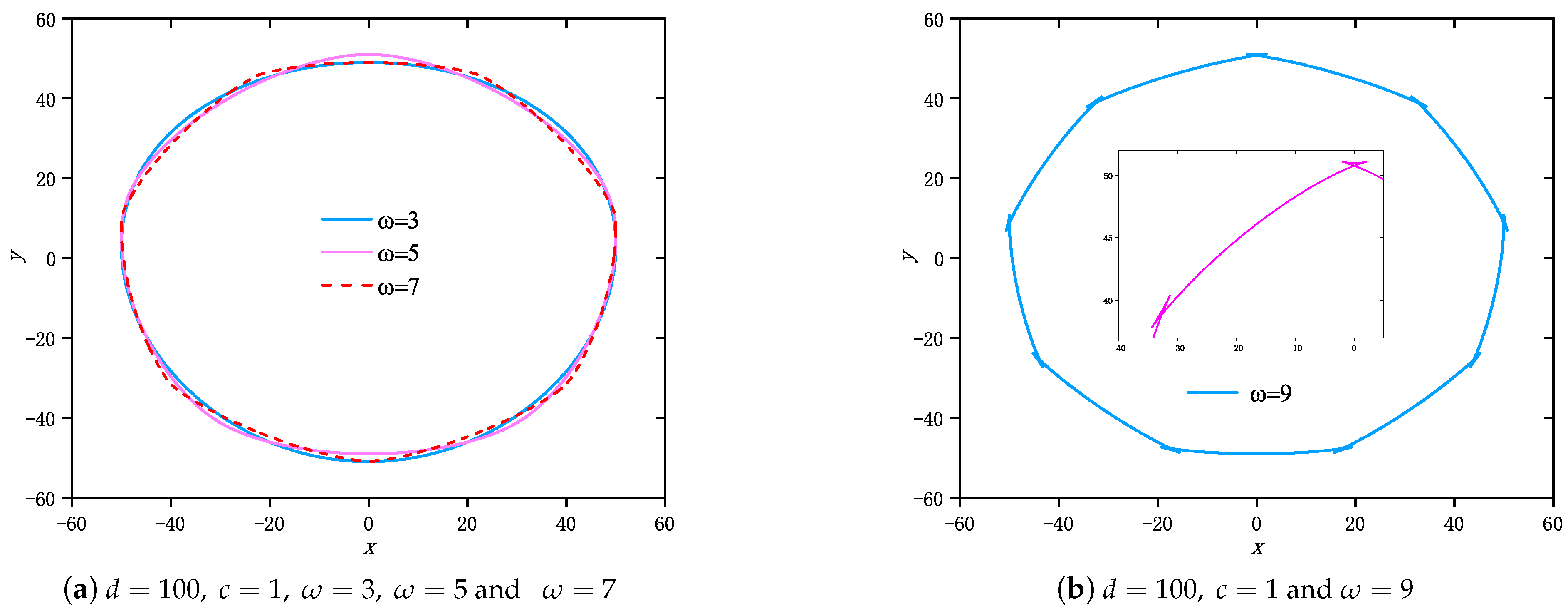
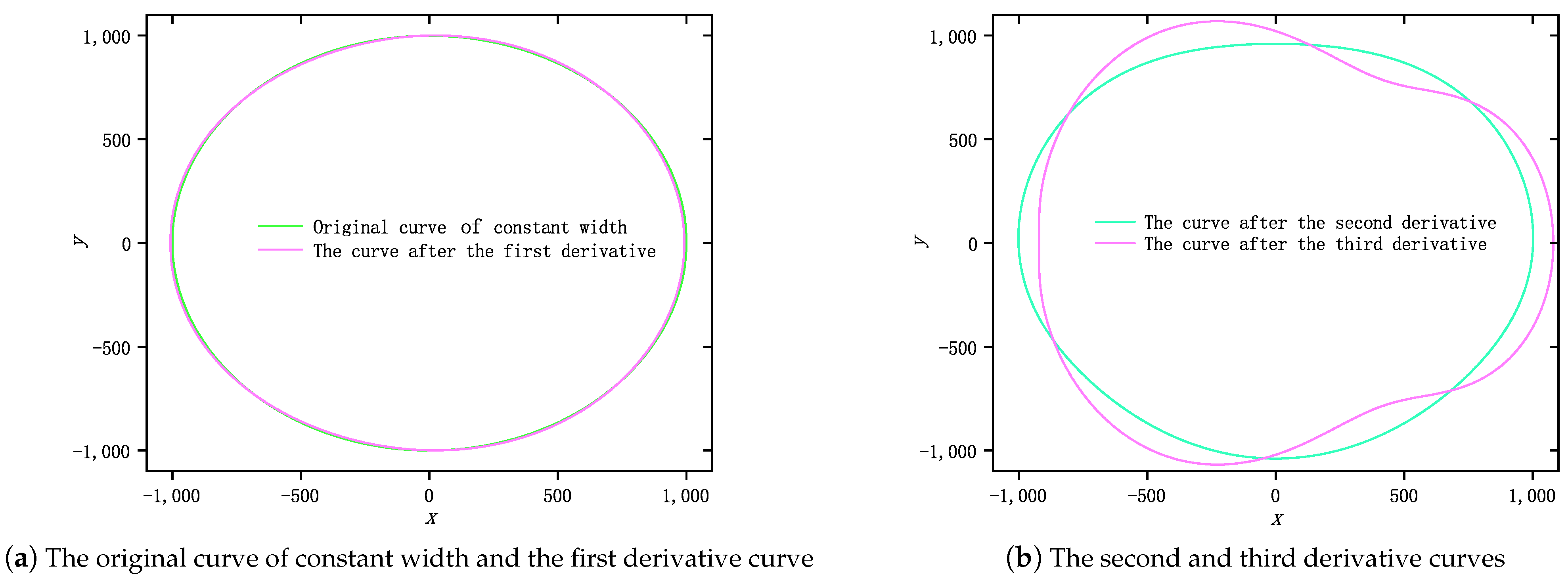
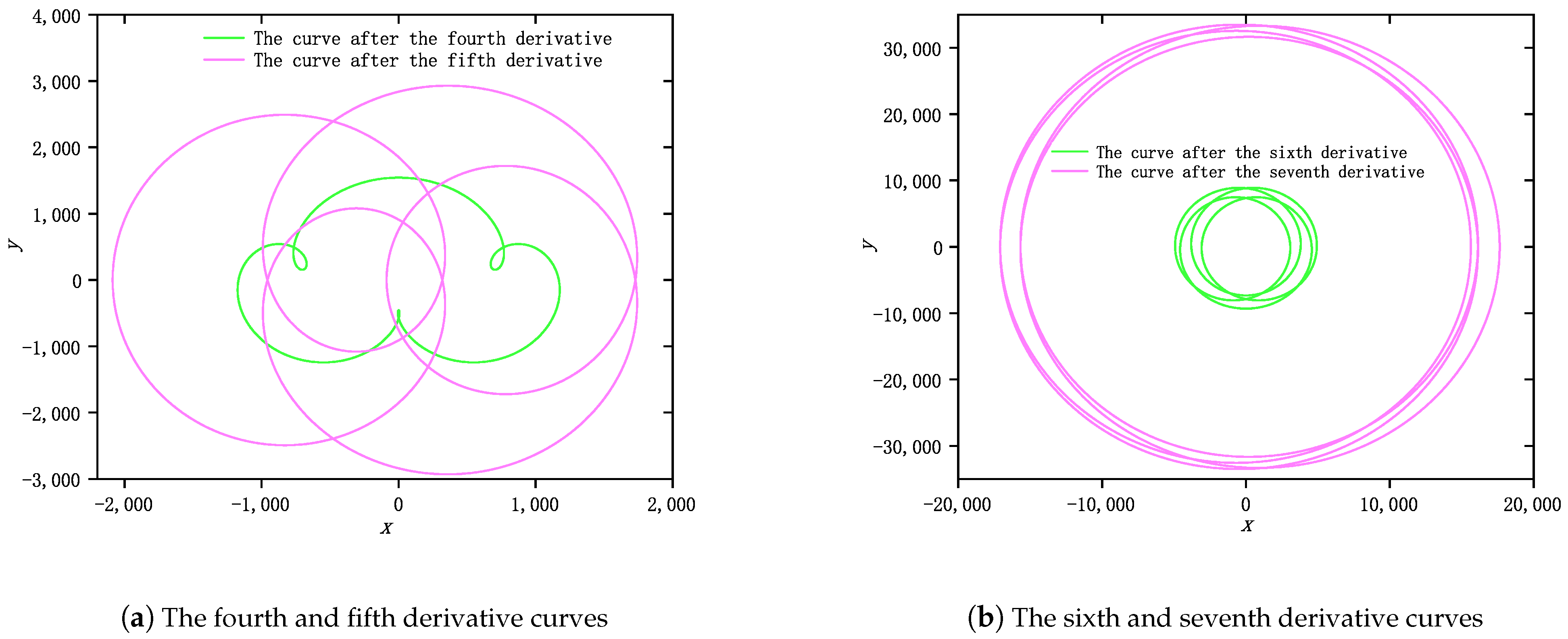
4. Simulation Results

In this section, we will present some simulation results to illustrate the main result of this paper.

First, for the support function (19), we set $C=1,d=100,\omega =3,5,7,9.$ When $\omega =3,5,7$, $\Gamma$ in (20) represents a smooth curve of constant width, respectively, as can be seen in Figure 1a. However, for $\omega =9$, since (18) is not satisfied, $\Gamma$ in (20) is not a simple closed convex curve according to Lemma 1, as depicted in Figure 1b.

To further illustrate the proposed result, we set $C=1,d=2000,\omega =3$ in (19) and take different derivative orders of (21). When the derivative order is less than 2, the curve after the corresponding derivative is still a curve of constant width, as shown in Figure 2a, as well as the blue line in Figure 2b. When the derivative order is equal to 3, the curve is no longer convex, as depicted in the purple line in Figure 2b. Moreover, if the derivative order is increasing, the obtained curve is able to intersect itself, and it is no longer a simple closed curve, as shown in Figure 3a. When the derivative order is continuously increased, the resulting curve is approximated to (24). Namely, the curve is a circle of radius $|\frac{C}{2}(1-\omega ){(\omega +1)}^n|$ that has turned four times, as shown in Figure 3b. In addition, when the derivative order is large enough, the four circles will overlap into one circle.

5. Conclusions

This paper innovatively introduces the characteristic equation of a time delay system to analyze the $C^{\infty }$ smooth curve of constant width. We can construct a $C^r$ smooth non-circular curve of constant width on the basis of the above analysis. We also prove that there is no $C^{\infty }$ smooth non-circular curve of constant width, which is still a curve of constant width after taking any number of derivatives.

References

1. Moon, Y.; Kota, S. Automated synthesis of mechanisms using dual-vector algebra. Mech. Mach. Theory 2002, 37, 143–166. [Google Scholar] [CrossRef]
2. Martini, H.; Mustafaev, Z. A new construction of curves of constant width. Comput. Aided Geom. Des. 2008, 25, 751–755. [Google Scholar] [CrossRef]
3. Borovikova, M.; Ibragimov, Z. Convex bodies of constant width and the Apollonian metric. Bull. Public Health Soc. 2008, 31, 117–128. [Google Scholar]
4. Groemer, H.; Wallen, L.J. A measure of asymmetry for domains of constant width. Beitr. Algebra Geom. 2001, 42, 517–521. [Google Scholar]
5. Rabinowitz, S. A polynomial curve of constant width. Mo. J. Math. Sci. 1997, 9, 3–27. [Google Scholar] [CrossRef]
6. Paciotti, L. Curves of constant width and their shadows. Whitman Sr. Proj. 2010, 2010, 20. [Google Scholar]
7. Xu, W.X.; Zhou, J.Z.; Chen, F.W. A kind of constant width “isosceles trapezoid”. Sci. China Math. 2011, 41, 855–860. [Google Scholar]
8. Yang, Y. A Convex Set of Constant Width with an Opposite Top Sector; Wuhan University of Science and Technology: Wuhan, China, 2015. [Google Scholar]
9. Mozgawa, W. Mellish theorem for generalized constant width curves. Aequ. Math. 2015, 89, 1095–1105. [Google Scholar] [CrossRef] [Green Version]
10. Mellish, A.P. Notes on differential geometry. Ann. Math. 1931, 32, 181–190. [Google Scholar] [CrossRef]
11. Resnikoff, H.L. On curves and surfaces of constant width. arXiv 2015, arXiv:1504.06733. [Google Scholar]
12. Kupitz, Y.; Martini, H.; Wegner, B. A linear-time construction of reuleaux polygons. Beitr. Algebra Geom. 1996, 37, 415–427. [Google Scholar]
13. Pan, S.L. An application of tangential polar coordinates. J. East China Norm. Univ. Nat. Sci. 2003, 1, 13–16. [Google Scholar]
14. Martini, H.; Montejano, L.; Oliveros, D. Sections of bodies of constant width. In Bodies of Constant Width; Birkhäuser: Cham, Switzerland, 2019. [Google Scholar]
Figure 1. Trajectory curves of (20) with different ω .
Mathematics 09 01131 g001
Figure 2. Trajectory curves with different number of derivatives ( d = 2000 , c = 1 , ω = 3 ).
Mathematics 09 01131 g002
Figure 3. Trajectory curves with different number of derivatives ( d = 2000 , c = 1 , ω = 3 ).
Mathematics 09 01131 g003
Publisher’s Note: MDPI stays neutral with regard to jurisdictional claims in published maps and institutional affiliations.