Level Sets of Weak-Morse Functions for Triangular Mesh Slicing

 , , and
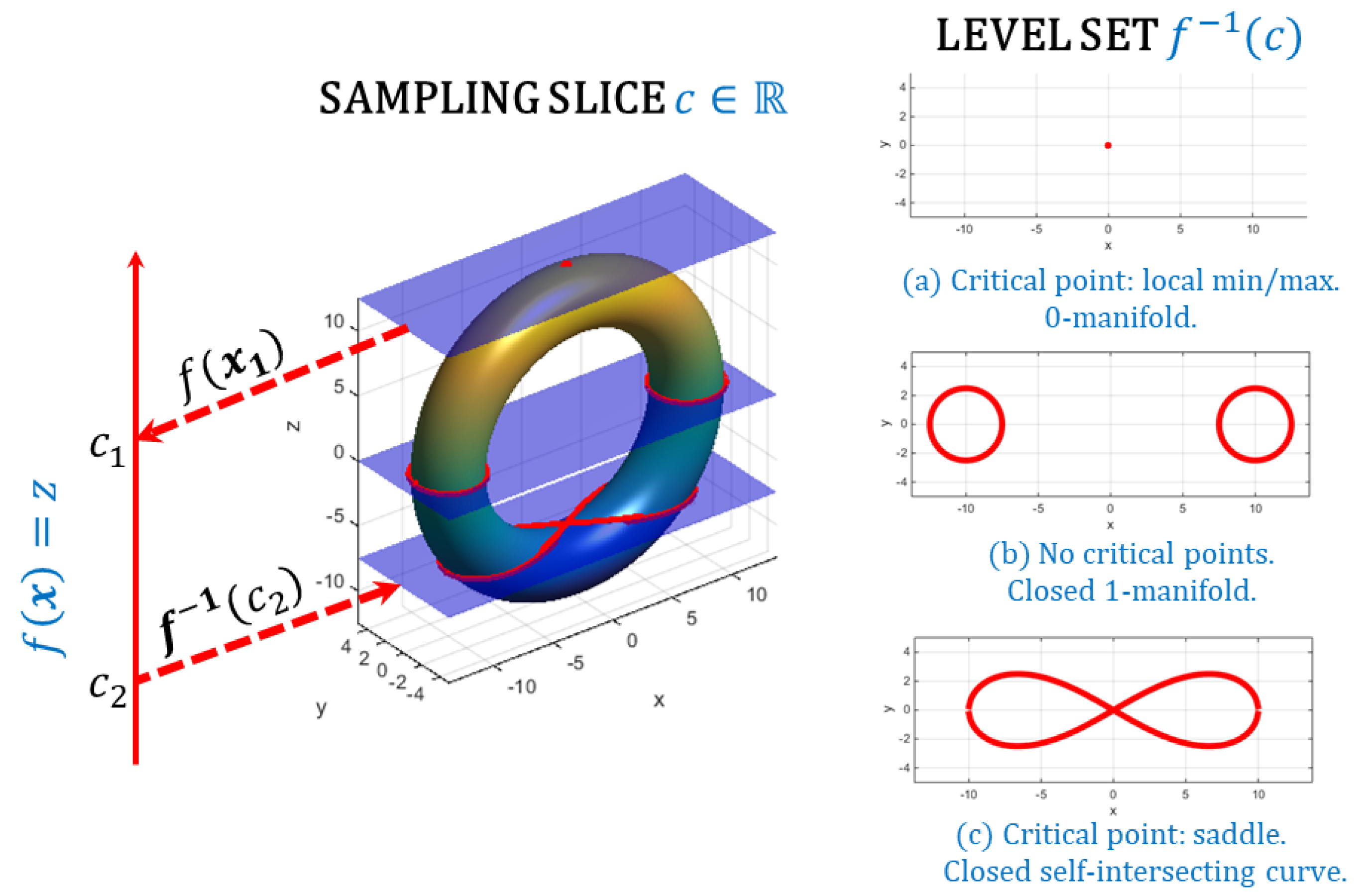
Abstract
:1. Introduction
2. Literature Review
2.1. Parallel-Planes Mesh Slicing
2.2. Non-Parallel-Planes Mesh Slicing
2.3. Conclusions of the Literature Review
3. Methodology
3.1. Mathematical Description of the Problem
3.1.1. Strong-Morse Function
3.1.2. Weak-Morse Function
3.1.3. Level Set Types
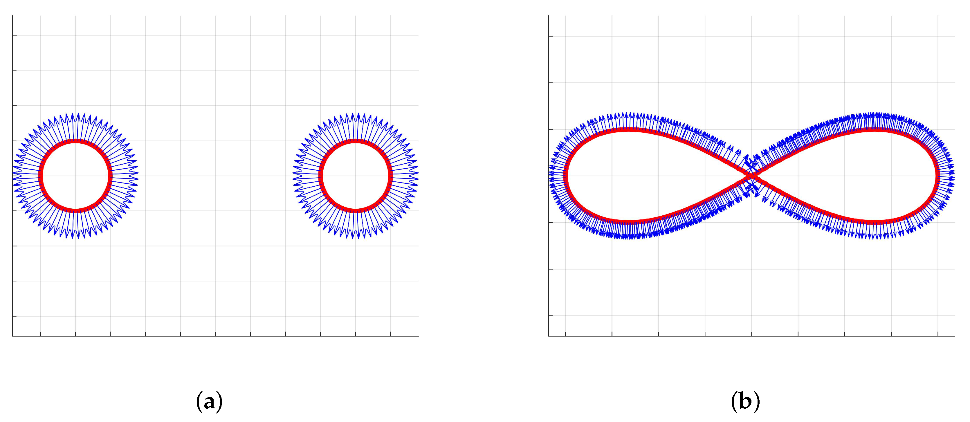
- Closed 1-manifold contour: contains no critical points:In this case defines a simple, oriented, closed curve (1-manifold homeomorphic to the unit circle).
- 0-manifold point: contains a strict local minimum (or maximum) :where, is a small neighborhood around the point x. Notice that for a local minimum (or maximum), . The level set corresponds to a 0-manifold isolated point .
- Non-degenerate saddle: contains a non-degenerate saddle point :in which, for a small neighborhood, :This contour locally produces a self intersecting (non-manifold), 1D curve with the shape of an “X” (see Figure 2).
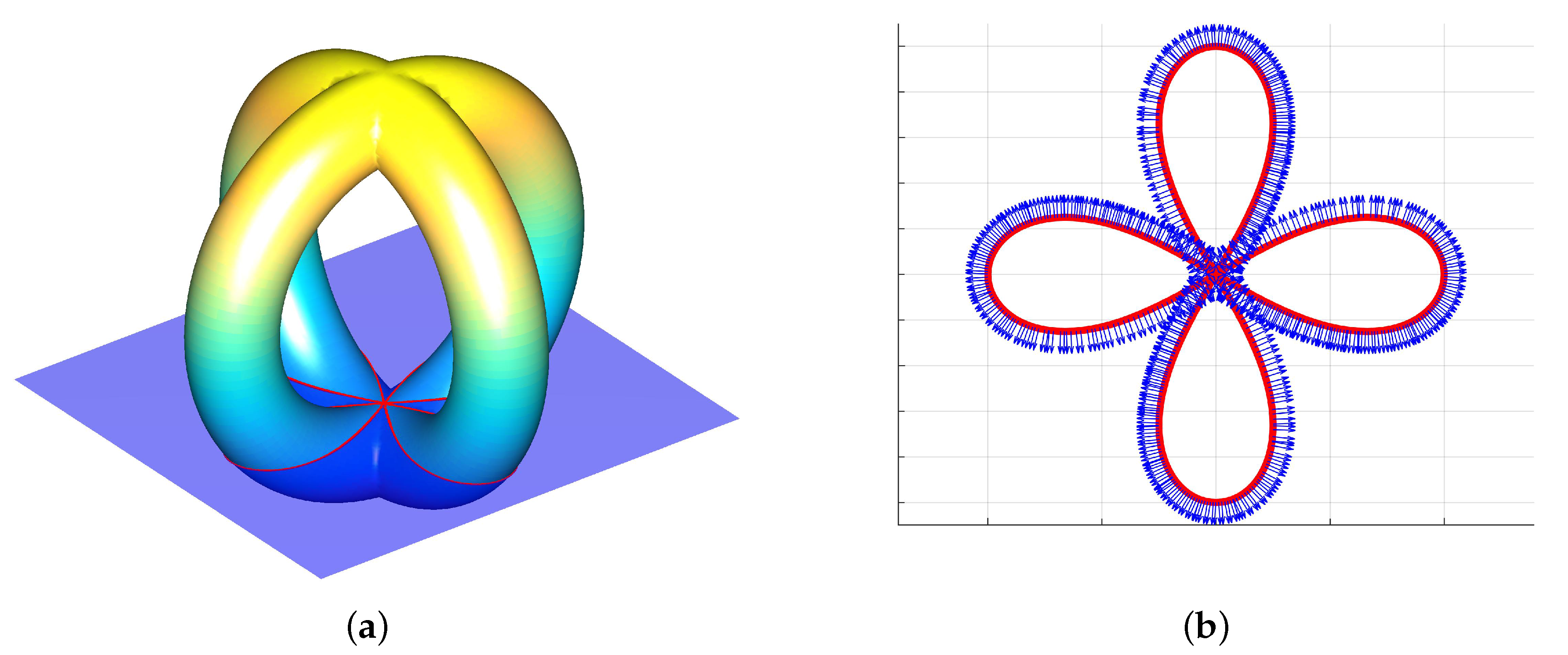
- Degenerate saddle: contains degenerate saddle point :then for a small neighborhood :Similar to the non-degenerate saddle, the degenerate saddle produces a self-intersecting curve with () 1-manifold branches (see Figure 2).
- Degenerate 1D region: contains a local minimum (or maximum) along a 1D path:andThis region defines a non-manifold 1D compact region, possibly with non-empty boundaries.
- Degenerate 2-Manifold region: contains a critical 2-manifold region:The region is locally homeomorphic to . The definition of locally homeomorphic permits the existence of holes in the region .
3.1.4. Contours Orientation
- Closed 1-manifold: The orientation of on the slicing plane is defined by the projection of the surface normal vector, that is:where is the vector normal to at x, and is the corresponding projection on the slicing plane.
- 0-manifold point: Not oriented.
- Non-degenerate saddle: The orientation of the non-degenerate saddle point is equally defined by the projection to the surface normal vector:for all .
- Degenerate saddle: Exactly the same as the non-degenerate saddle case.
- Degenerate 1D region: Not oriented.
- Degenerate 2-manifold region: Not oriented in the slicing plane. However, the boundary is an oriented, closed 1-manifold embedded in .
3.2. Slicing Algorithm
- is the set of all closed and oriented polylines on the slicing plane. The set includes closed 1-manifolds and saddle points with its adjacent neighborhoods
- is the 0-manifold set of all local minima/maxima vertices in M that lie on the slicing plane.
- is the set of all non-oriented (and possibly with border) contours on the slicing. includes all degenerate 1D regions of M.
- is the set of all 2-manifold regions (triangles) in M that lie on the slicing plane.
- Degenerate 2-manifold region: Let . if:
- Degenerate 1D region: Let , such that . is a degenerate 1D region if:where is the z-coordinate of the vertex that is opposite to the oriented edge .
- Degenerate and non-degenerate saddle: Let , . is a saddle point if:where maps each vertex to the set of all triangles that are incident to it. Therefore, is the set of all triangles that intersect the slicing plane and is the number of segments in the triangle/plane intersections in such a set.
- 0-manifold point: Let , . is a local minimum (or maximum) if:where maps each vertex to the set of all vertices that are adjacent to it.
- Closed 1-manifold: Let , . The edge if:with and being one of the triangle t edges that intersect the plane . It is worth noting that not necessarily belongs to the vertex set X.
| Algorithm 1 Slice triangular mesh. |
| Require:, |
| Ensure: |
| 1: for do |
| 2: |
| 3: if then |
| 4: push(F,t) |
| 5: end if |
| 6: end for |
| 7: for do |
| 8: if then |
| 9: |
| 10: |
| 11: if then |
| 12: push(, ) |
| 13: end if |
| 14: end if |
| 15: end for |
| 16: for do |
| 17: is_min ← TRUE |
| 18: is_max ← TRUE |
| 19: for do |
| 20: if then |
| 21: is_max ← FALSE |
| 22: end if |
| 23: if then |
| 24: is_min ← FALSE |
| 25: end if |
| 26: end for |
| 27: if is_min ∨ is_max then |
| 28: push(P,) |
| 29: end if |
| 30: end for |
| 31: for do |
| 32: |
| 33: if then |
| 34: |
| 35: if then |
| 36: swap(, ) |
| 37: end if |
| 38: push() |
| 39: end if |
| 40: end for |
| 41: return |
4. Results
4.1. Weak-Morse Slicing
4.2. Applications in Additive Manufacturing
5. Conclusions
Author Contributions
Funding
Conflicts of Interest
Abbreviations
| A closed 2-manifold embedded in . | |
| f | A scalar function . In this manuscript, is the height function, named also as the slicing function. |
| Level sets of the function f. . | |
| Scalar that defines the slicing plane. is the slicing plane at . | |
| For any , is the tangent plane of at x. | |
| Gradient operator defined on the surface (tangent planes) of . . | |
| Hessian matrix defined on the surface (tangent planes) of . . | |
| strong-Morse | A strong-Morse (or simply Morse) function f, is a function in which all of its critical points are non-degenerate. A critical point is degenerate if . |
| weak-Morse | Denomination used exclusively for the purpose of this manuscript. f is weak-Morse if there exists a finite set of values (each corresponding to a cross cut of ) where is degenerate (i.e., non-Morse). f satisfies Morse criteria elsewhere. |
| Vector normal to the tangent plane . . | |
| Projection of the vector onto the slicing plane. . | |
| Small neighborhood in around the point . | |
| M | 2-manifold triangular mesh , which is a piecewise linear discretization of . is the set of mesh vertices (geometry), and is the set of mesh triangles (topology). |
| E | Set of bidirectional edges that belong to the graph of the mesh M. if for any k, . |
| Set of all vertices that are adjacent to the vertex . . | |
| Set of all triangles that are incident to the vertex . . | |
| Slicing function defined on the triangular mesh M. . | |
| Set of all oriented and closed polylines in for a given slice c of M. . | |
| P | 0-manifold set of all local minima/maxima vertices of M that lie on the slicing plane. . |
| Set of all non-oriented compact (i.e., possibly with borders) polylines in for a given slice c of M. . | |
| F | Set of all 2-manifold regions (triangles) in M that lie on the slicing plane. . |
References
- Ding, D.; Pan, Z.; Cuiuri, D.; Li, H.; van Duin, S. Advanced Design for Additive Manufacturing: 3D Slicing and 2D Path Planning. In New Trends in 3D Printing; Shishkovsky, I.V., Ed.; IntechOpen: Rijeka, Croatia, 2016; Chapter 1. [Google Scholar] [CrossRef] [Green Version]
- Zhao, D.; Guo, W. Shape and Performance Controlled Advanced Design for Additive Manufacturing: A Review of Slicing and Path Planning. J. Manuf. Sci. Eng. 2019, 142, 010801. [Google Scholar] [CrossRef]
- Mejia-Parra, D.; Sánchez, J.R.; Ruiz-Salguero, O.; Alonso, M.; Izaguirre, A.; Gil, E.; Palomar, J.; Posada, J. In-Line Dimensional Inspection of Warm-Die Forged Revolution Workpieces Using 3D Mesh Reconstruction. Appl. Sci. 2019, 9, 1069. [Google Scholar] [CrossRef] [Green Version]
- Sánchez, J.R.; Segura, Á.; Barandiaran, I. Fast and accurate mesh registration applied to in-line dimensional inspection processes. Int. J. Interact. Des. Manuf. 2018, 12, 877–887. [Google Scholar] [CrossRef]
- Steuben, J.C.; Iliopoulos, A.P.; Michopoulos, J.G. Implicit slicing for functionally tailored additive manufacturing. Comput. Aided Des. 2016, 77, 107–119. [Google Scholar] [CrossRef]
- Jin, Y.; He, Y.; Fu, G.; Zhang, A.; Du, J. A non-retraction path planning approach for extrusion-based additive manufacturing. Robot. Comput. Integr. Manuf. 2017, 48, 132–144. [Google Scholar] [CrossRef]
- Jin, Y.; Du, J.; He, Y. Optimization of process planning for reducing material consumption in additive manufacturing. J. Manuf. Syst. 2017, 44, 65–78. [Google Scholar] [CrossRef]
- Nilsiam, Y.; Sanders, P.; Pearce, J.M. Slicer and process improvements for open-source GMAW-based metal 3-D printing. Addit. Manuf. 2017, 18, 110–120. [Google Scholar] [CrossRef] [Green Version]
- Budinoff, H.; McMains, S. Prediction and visualization of achievable orientation tolerances for additive manufacturing. In Proceedings of the 15th CIRP Conference on Computer Aided Tolerancing, CIRP CAT, Milan, Italy, 11–13 June 2018. [Google Scholar] [CrossRef]
- Campocasso, S.; Chalvin, M.; Reichler, A.K.; Gerbers, R.; Droder, K.; Hugel, V.; Dietrich, F. A framework for future CAM software dedicated to additive manufacturing by multi-axis deposition. In Proceedings of the 6th CIRP Global Web Conference—Envisaging the Future Manufacturing, Design, Technologies and Systems in Innovation Era (CIRPe2018), 23–25 October 2018; Available online: http://www.cirpe2018.org/ (accessed on 17 September 2020). [CrossRef]
- Michel, F.; Lockett, H.; Ding, J.; Martina, F.; Marinelli, G.; Williams, S. A modular path planning solution for Wire + Arc Additive Manufacturing. Robot. Comput. Integr. Manuf. 2019, 60, 1–11. [Google Scholar] [CrossRef]
- Roschli, A.; Gaul, K.T.; Boulger, A.M.; Post, B.K.; Chesser, P.C.; Love, L.J.; Blue, F.; Borish, M. Designing for Big Area Additive Manufacturing. Addit. Manuf. 2019, 25, 275–285. [Google Scholar] [CrossRef]
- Ma, W.; But, W.C.; He, P. NURBS-based adaptive slicing for efficient rapid prototyping. Comput. Aided Des. 2004, 36, 1309–1325. [Google Scholar] [CrossRef]
- Alexa, M.; Hildebrand, K.; Lefebvre, S. Optimal Discrete Slicing. ACM Trans. Graph. 2017, 36. [Google Scholar] [CrossRef] [Green Version]
- Mao, H.; Kwok, T.H.; Chen, Y.; Wang, C.C. Adaptive slicing based on efficient profile analysis. Comput. Aided Des. 2019, 107, 89–101. [Google Scholar] [CrossRef]
- Gregori, R.M.M.H.; Volpato, N.; Minetto, R.; Silva, M.V.G.D. Slicing Triangle Meshes: An Asymptotically Optimal Algorithm. In Proceedings of the 14th International Conference on Computational Science and Its Applications, Guimaraes, Portugal, 30 June–3 July 2014; pp. 252–255. [Google Scholar]
- Minetto, R.; Volpato, N.; Stolfi, J.; Gregori, R.M.; da Silva, M.V. An optimal algorithm for 3D triangle mesh slicing. Comput. Aided Des. 2017, 92, 1–10. [Google Scholar] [CrossRef]
- Xu, J.; Hou, W.; Sun, Y.; Lee, Y.S. PLSP based layered contour generation from point cloud for additive manufacturing. Robot. Comput. Integr. Manuf. 2018, 49, 1–12. [Google Scholar] [CrossRef]
- Gohari, H.; Barari, A.; Kishawy, H. Using Multistep Methods in Slicing 2 1/2 Dimensional Parametric Surfaces for Additive Manufacturing Applications. In Proceedings of the 2th IFAC Workshop on Intelligent Manufacturing Systems IMS 2016, Austin, TX, USA, 5–7 December 2016. [Google Scholar] [CrossRef]
- Song, Y.; Yang, Z.; Liu, Y.; Deng, J. Function representation based slicer for 3D printing. Comput. Aided Geom. Des. 2018, 62, 276–293. [Google Scholar] [CrossRef]
- Feng, J.; Fu, J.; Lin, Z.; Shang, C.; Niu, X. Layered infill area generation from triply periodic minimal surfaces for additive manufacturing. Comput. Aided Des. 2019, 107, 50–63. [Google Scholar] [CrossRef]
- Luu, T.H.; Altenhofen, C.; Ewald, T.; Stork, A.; Fellner, D. Efficient slicing of Catmull-Clark solids for 3D printed objects with functionally graded material. Comput. Graph. 2019, 82, 295–303. [Google Scholar] [CrossRef]
- Messner, M.C. A fast, efficient direct slicing method for slender member structures. Addit. Manuf. 2017, 18, 213–220. [Google Scholar] [CrossRef]
- Hu, J. Study on STL-Based Slicing Process for 3D Printing. In Proceedings of the 28th Annual International Solid Freeform Fabrication Symposium—An Additive Manufacturing Conference, Austin, TX, USA, 7–9 August 2017; pp. 885–895. [Google Scholar]
- Hildebrand, K.; Bickel, B.; Alexa, M. Orthogonal slicing for additive manufacturing. Comput. Graph. 2013, 37, 669–675. [Google Scholar] [CrossRef]
- Murtezaoglu, Y.; Plakhotnik, D.; Stautner, M.; Vaneker, T.; van Houten, F.J. Geometry-Based Process Planning for Multi-Axis Support-Free Additive Manufacturing. In Proceedings of the 6th CIRP Global Web Conference—Envisaging the Future Manufacturing, Design, Technologies and Systems in Innovation Era (CIRPe 2018), 23–25 October 2018; Available online: http://www.cirpe2018.org/ (accessed on 17 September 2020). [CrossRef]
- Ding, D.; Pan, Z.; Cuiuri, D.; Li, H.; Larkin, N.; van Duin, S. Automatic multi-direction slicing algorithms for wire based additive manufacturing. Robot. Comput. Integr. Manuf. 2016, 37, 139–150. [Google Scholar] [CrossRef]
- Ezair, B.; Fuhrmann, S.; Elber, G. Volumetric covering print-paths for additive manufacturing of 3D models. Comput. Aided Des. 2018, 100, 1–13. [Google Scholar] [CrossRef]
- Jin, Y.; Du, J.; He, Y.; Fu, G. Modeling and process planning for curved layer fused deposition. Int. J. Adv. Manuf. Technol. 2017, 91, 273–285. [Google Scholar] [CrossRef]
- Zhao, D.; Guo, W. Mixed-layer adaptive slicing for robotic Additive Manufacturing (AM) based on decomposing and regrouping. J. Intell. Manuf. 2019, 31, 985–1002. [Google Scholar] [CrossRef]
- Banchoff, T.F. Critical Points and Curvature for Embedded Polyhedral Surfaces. Am. Math. Mon. 1970, 77, 475–485. [Google Scholar] [CrossRef]
- Forman, R. Morse Theory for Cell Complexes. Adv. Math. 1998, 134, 90–145. [Google Scholar] [CrossRef] [Green Version]
- Fugacci, U.; Landi, C.; Varli, H. Critical sets of PL and discrete Morse theory: A correspondence. Comput. Graph. 2020, 90, 43–50. [Google Scholar] [CrossRef]
- Vatti, B.R. A Generic Solution to Polygon Clipping. Commun. ACM 1992, 35, 56–63. [Google Scholar] [CrossRef]
- Regli, W.C.; Foster, C.; Hayes, E.; Ip, C.Y.; McWherter, D.; Peabody, M.; Shapirsteyn, Y.; Zaychik, V. National Design Repository: A Status Report. In Proceedings of the International Joint Conferences on Artificial Intelligence (IJCAI) and AAAI/SIGMAN Workshop on AI in Manufacturing Systems, Seattle, WA, USA, 4–10 August 2001. [Google Scholar]


© 2020 by the authors. Licensee MDPI, Basel, Switzerland. This article is an open access article distributed under the terms and conditions of the Creative Commons Attribution (CC BY) license (http://creativecommons.org/licenses/by/4.0/).
Share and Cite
Mejia-Parra, D.; Ruiz-Salguero, O.; Cadavid, C.; Moreno, A.; Posada, J. Level Sets of Weak-Morse Functions for Triangular Mesh Slicing. Mathematics 2020, 8, 1624. https://doi.org/10.3390/math8091624
Mejia-Parra D, Ruiz-Salguero O, Cadavid C, Moreno A, Posada J. Level Sets of Weak-Morse Functions for Triangular Mesh Slicing. Mathematics. 2020; 8(9):1624. https://doi.org/10.3390/math8091624
Chicago/Turabian StyleMejia-Parra, Daniel, Oscar Ruiz-Salguero, Carlos Cadavid, Aitor Moreno, and Jorge Posada. 2020. "Level Sets of Weak-Morse Functions for Triangular Mesh Slicing" Mathematics 8, no. 9: 1624. https://doi.org/10.3390/math8091624