1. Introduction
Computer games are referred to as the “fruit flies” of the discipline of artificial intelligence (AI) [
1] with broad applications in areas such as robotics [
2], control theory [
3], social networks [
4], etc. Various game models have been developed for characterizing different strategic decision-making scenarios, e.g., the Cournot Model for quantity competition, Stackelberg game theory for asymmetric competition [
5], or the negotiation model with a certain degree of cooperation [
6]. With equilibrium concepts, game theory provides a way of predicting and analysing the optimal strategies in game-like scenarios [
7], and provides inspiring ideas for other fields where the solutions to the problems can be obtained via game-theoretic optimal strategies [
8]. For instance, the generative adversarial networks (GANs) [
9] used in AI are essentially holding a competitive game between two neural networks, in which they continuously optimize themselves and finally converge to the Nash equilibrium.
As an important avenue of computer game research, the study of zero-sum games [
10,
11] involves knowledge representations, game-tree search algorithms, state evaluation functions, etc. To determine what action a player should take to win a game, an appropriate game-tree search algorithm that can search and analyze the game tree for the game of interest is of great importance. In a game tree [
12] (such as shown in
Figure 1), the nodes and branches represent the possible situations and moves, respectively. Specifically, the root node represents the current board state, and its child nodes represent all future states that could be reached after the corresponding moves. Each leaf node represents a possible final board state of the game.
One commonly used adversarial search algorithm is the minimax algorithm [
13]. This has been widely applied in practical systems, such as the chess program Deep Blue, which defeated the world champion Kasparov in 1997 [
14,
15], and has inspired the design of many algorithms in search domains, such as iterative deepening (IDA*) [
16], real-time search (RTA*) [
17] and bidirectional search [
18], etc.
Theoretically, this algorithm can obtain the optimal solution to a zero-sum game with complete information on the premise that the whole game tree is available. However, due to the tremendous size of the state space and limitations on the computational capabilities, it is typically impossible to completely search the game tree. Therefore, in any practical application, the game tree will be extended only to a certain finite depth d. Statistic heuristic functions will be used to evaluate the state values of the nodes of depth d, while the values of other nodes of depths less than d are computed in accordance with the minimax rule.
Refinements to this algorithm have been developed to address various concerns, in particular to improve the efficiency. As the complexity of minimax mainly depends on the tree depth and the branching factor, the main direction is attempting to reduce these two parameters. There are two methods to reduce the tree depth: a function approximation, i.e., to estimate the goodness of a situation by constructing an evaluation function [
19], and a simulation-based roll-out [
20], i.e., using a relatively simple game strategy to quickly come to the end. The basic way to reduce the branching factor is pruning. The most famous ones are alpha-beta pruning [
21,
22] and Monte Carlo simulations [
23] (which first estimate a prior probability distribution
P, and then sample part of the path according to
P for estimation).
However, except for the efficiency of the search algorithm, another issue that should be considered is the accuracy. The incomplete exploration of the game tree and inaccuracy in the evaluation of game situations may hinder the decision accuracy of the minimax algorithm. All these studies are based on the assumption that deeper searches typically lead to better performance. In fact, this assumption has been questioned in the literature [
24]. The authors in [
25,
26] first showed that, for certain classes of game trees, the decision quality was degraded by searching deeper and backing up the heuristic values using the minimax propagation rule. They called this phenomenon game-tree pathology [
25,
27]. Sadikov [
28] similarly concluded from a King-Rook-King (KRK) chess endgame experiment that the evaluation accuracy might decrease with increasing search depth, thus, confirming the pathological phenomenon of the minimax algorithm.
To overcome the impact of such pathological nodes on the game-tree search process, appropriate refinements to the standard minimax algorithm need to be developed. In recent years, the error minimizing minimax (EMM) algorithm was proposed to reduce the impact of pathological nodes on the search quality [
29,
30] by estimating different node types and addressing them separately. However, in some game scenarios, it is not guaranteed that the estimation of the node type is correct. In addition, estimating the node types introduces extra complexity to the search process.
With the present work, we would like to move the stance further by presenting a novel refinement of the minimax algorithm, called the iterative optimal minimax (IOM) algorithm. The main idea is to improve the backup rule for the heuristic values of the states. In this algorithm, the state values of the nodes in each layer of the game tree are comprehensively considered. During the process of extending the game tree, a static heuristic function is used to evaluate the state value of each node, which is called its evaluation value, . Then, the initial values of the nodes are updated from the leaves to the root, following the backup rule -, where for any node A, denotes the backup value of A, denotes the evaluation value of A, and denotes the minimum among the backup values of A’s children .
In the process of updating the state values, the maximum backup value is selected as the final backup value for any MAX layer node, while the minimum backup value is selected for any MIN layer node. This approach not only reduces the influence of pathological nodes on the decision quality but also avoids the high complexity of the EMM algorithm. We also incorporate a pruning strategy to enhance the efficiency of the IOM algorithm in practice.
Experiments were conducted on the games of chess and gobang [
31], which are two classical competition games in which players’ final payoffs reflect their decision quality. The experimental results show that the proposed IOM algorithm outperformed the standard minimax and EMM algorithms with regard to the decision quality.
The remainder of this paper is organized as follows. In
Section 2, we present some preliminaries that are essential to the understanding of the proposed algorithm. In
Section 3, we introduce our IOM algorithm, including the underlying idea, the execution procedure, and the related complexity issues.
Section 4 is devoted to the experiments on chess and gobang. This work is concluded in
Section 5.
2. Preliminaries
The minimax algorithm is a classical game-tree search algorithm that can be used to solve many zero-sum game problems. A deeper search is generally considered to yield a more accurate evaluation of the goodness of the game states. However, we also recognize that in the presence of pathological nodes, both the evaluation quality and the decision quality may decline with a deeper search. This section recalls some preliminaries, including the details of the minimax algorithm, the occurrence of pathological nodes, and the EMM algorithm.
2.1. Minimax
For a zero-sum game with perfect information, one of the most popular game-solving methods is the minimax algorithm. We assumed that both sides of the game follow the principle of minimizing the maximum benefit of the other while maximizing their own benefit; this is why the algorithm is named minimax. For a sufficiently complex game, the game tree is extended only to a certain finite depth, and a heuristic evaluation function is used to evaluate the state value of each leaf node. Then, from the leaf nodes, the state values of the upper-level nodes are calculated in accordance with the minimax backup rule until the state value of the root node is obtained. Among all child nodes of the root node, the one with the highest state value is taken as the best option in the current state.
The negamax algorithm is a variant of the minimax algorithm that relies on the fact that in a zero-sum game to simplify the implementation of the algorithm. As most adversarial search engines use some form of negamax algorithm for coding, the algorithm implementation presented in this paper also adopts the negamax form. The target is to find the node value for the player who is playing at the root node. First, the evaluation values of the leaf nodes are calculated using the evaluation function. Then, the inverse of each of these evaluation values is taken and transmitted in the bottom-up direction through the tree, layer by layer, until the value of the root node is obtained. During this backward updating process, each upper-level node inherits the maximum value among the backup values of its children.
Figure 2 illustrates the search process of the negamax algorithm in a game tree with a depth of 3. In this example, node
A is the root node of the game tree, where it is player
A’s turn to move. Finally, the value of root node
A is found to be 9 through a minimax search, and the immediate child node with the best evaluation value, node
C, is selected as the best move at the root node.
2.2. Pathological Node Analysis
For nonterminal nodes, errors are inevitable when evaluating the values of nodes in a game tree using a heuristic evaluation function. When the negamax backup rule is used for value propagation, different types of nodes show distinct error probabilities. In general, there are three representative types of nodes. We consider the three simple game trees shown in
Figure 3, where each node represents a game state, and the number inside each leaf node is its evaluation value, while the number inside the root node is the backup value propagated from its child nodes. The root nodes correspond to the three different node types, and the values 1 and −1 indicate that the player would win or lose the game in that state, respectively.
A node of type I is evaluated as a guaranteed winning position. The evaluation of the parent node will be incorrect only if all child nodes are calculated incorrectly. From a node of type II, it is possible to win the game. The parent node will be evaluated incorrectly if the evaluations for the child nodes of value −1 are incorrect while the evaluations for the child nodes of value 1 are correct. At a node of type III, the player is thought to be guaranteed to lose the game. However, the evaluation of this node will be erroneous if any of its child nodes is not evaluated correctly. Let the error probability when evaluating the state value of a node via the static evaluation function be
e; then, the probability of returning an incorrect value for the predecessor node depends on its type:
In Equation (
1), since for any node with type I, an incorrect value is returned when the evaluations of both of its two successors are incorrect, the probability
of returning an incorrect value for the
I-node is
; Similarly, in Equation (
2), the probability
of returning an incorrect value for the
-node is obtained based on the probability
e of an incorrect evaluation of the successor of value −1 and the probability
of a correct evaluation of the successor of value 1. The case for type III can be derived in the same manner according to the features of this type.
Figure 4 shows curves characterizing the relationships between the error probability for the evaluation values of the leaves and for the backup value of the predecessor in the above three cases. To facilitate a comparison of the dynamic trends of these curves, a curve representing
is also presented in this figure. From this figure, it is only for a node of type III that the error probability at the predecessor is higher than the original error probability of the evaluation function.
2.3. Emm Algorithm
The EMM algorithm is a search algorithm proposed to handle the evaluation of pathological nodes (type III) in a game tree. By keeping track of the error probabilities of both the evaluation and backup values, this algorithm naturally distinguishes between pathological nodes (type III) and nonpathological nodes (types I or II). If the evaluation value allows a tighter error bound than the backup value, then the evaluation value will be taken as the final state value.
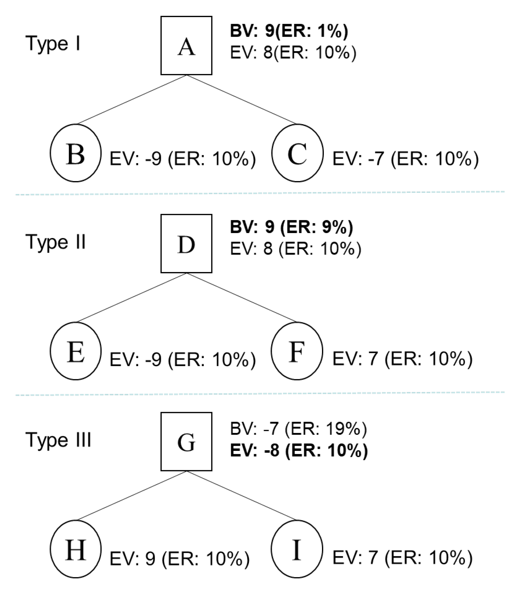
To illustrate this idea, we take the game tree shown in
Figure 5 as an example. For each leaf node, the evaluation value is given—the error probability of which is assumed to be 10%. For each root node, both the evaluation value and the backup value are calculated. In this figure, EV represents the evaluation value (
) of a node, and BV represents the backup value (
) of the node. ER denotes the error probability for each value.
Node A is of type I, and the error probability of its evaluation value is also 10%, while that of its backup value is 10% ∗ 10% = 1%. Therefore, the backup value is taken as the final state value of A. Node D is of type II. We concluded that the error probability of its backup value was 9% (node F will be correctly evaluated with a probability of 90%, while node E will be evaluated incorrectly with a probability of 10%). Therefore, the backup value is also selected for node B. However, for node G, which is of type III, the error probability of its backup value is 1 − (1 − 10%) = 19%. Hence, the evaluation value will be selected for this node.
3. Iterative Optimal Minimax (Iom)
A deeper minimax search can yield a higher decision quality. However, due to the existence of pathological nodes, updating the node values via backward induction from the leaf nodes in the minimax algorithm appears to not always be reliable, and thus, the decision quality of the search algorithm is affected. Although the EMM proposes a solution to the pathological phenomenon, that search algorithm still has many defects. In this section, we propose the IOM algorithm by improving the backup rule of the minimax algorithm. To increase the efficiency, we also present a pruning method for the basic IOM algorithm.
3.1. Main Idea
For the EMM algorithm, since the node type can be judged only after searching all child nodes of the target node during the search process, the time complexity of the algorithm is high and difficult to reduce. At the same time, the imprecision of the evaluation function can lead to incorrectness in determining the node type, giving rise to further errors during the propagation process.
In a game tree where the state values of the nodes are determined using a static evaluation function, there are errors in the state values of both the leaf and intermediate nodes. As we have seen, for a non-pathological node, the value resulting from the backward search of its children is more accurate, while for a pathological node, the value according to the static evaluation function is better. Note that the proportion of pathological nodes varies among different game trees. Typically, there are far fewer pathological nodes in a game tree than non-pathological nodes, and thus, the decision quality of a minimax search improves with increasing depth. However, if the pathological problem can be solved, a higher decision quality can be achieved.
To solve the local pathological problems that exist in a game tree and to avoid the shortcomings of the EMM algorithm, we propose the IOM algorithm by refining the backup rule of the minimax algorithm. The main idea is that calculating the state values of the intermediate nodes should involve not only the static evaluation function but also a search into the future, where these two aspects are given different weights. During the process of updating the state value of a node, the adopted backup rule can be expressed as , where for any node A, denotes the backup value of A, denotes the evaluation value of A, and denotes the minimum value among the backup values of A’s children.
This backup rule not only maintains the idea of the minimax algorithm by using the state values calculated using the static evaluation function but also reduces the influence of pathological nodes and yields a more accurate state value for the current node based on a search of the child nodes. Compared with the EMM algorithm, the proposed algorithm avoids potential errors in the evaluation on the node types and allows a tree pruning method to be incorporated into the process of searching the game tree to reduce the algorithm complexity.
3.2. Algorithm Description and Theoretical Effectiveness
The IOM algorithm first computes the static evaluation function for any given node. Then, the final value of each node is updated via a backpropagation manner in accordance with the backup rule, i.e., the final backup value of each node is equal to its evaluation value minus double the minimum backup value among its children.
Before presenting the full description of the IOM algorithm, we first illustrate the backup process via a short example, as shown in
Figure 6. This game tree is the same as shown in
Figure 2, except that the evaluation values of the non-leaf nodes are increased. The state value of a node, represented by the evaluation value
, is calculated via a static heuristic evaluation function from the perspective of the player-to-move. When the child nodes
D and
E have both been searched, the algorithm can obtain the minimum backup value
among
B’s children, i.e., 7 in this example.
According to the IOM backup rule, the backup value of B is then = −23. In the same way, we can obtain the backup value of node C as -22. These two values will then be propagated to node A in accordance with the backup rule . Thus, the backup value of is 53, and the optimal choice for the player at A is branch B. In this example, the IOM algorithm and the minimax algorithm yield different search results because the evaluation values of nodes B and C are quite different from the backup values they obtain from their children.
Via an iterative computation, we can find the following:
The above observation suggests that the final state value of the root depends on the evaluation values of all nodes on the optimal path following it, where the deeper the node is, the greater the weight of its evaluation value. By contrast, in the classical minimax algorithm, the backup value of each node depends only on the evaluation values of the leaf nodes.
More generally, we have the following theorem.
Theorem 1. Let G be a game tree rooted at R, where each node s has a set of moves, ms, for the player-to-move . Each node s is assigned an evaluation value . Let , with , be a sequence of nodes representing an optimal path computed using the IOM algorithm. Then, the following relationship holds.
= .
Proof. By induction on the length l of .
Base case: when , R is also a terminal node. It can be trivially seen that = . When , = . According to the IOM backup rule that = , it has that = since is the only child of . Induction assumption: for , the theorem holds. Induction: , = . Then, the path is a path of length m. Hence, = by the induction assumption. Since is an optimal path returned by IOM, it follows that = . Therefore, it holds that = = = . □
The above schema explains why our algorithm is more robust than the minimax and EMM algorithms. In IOM, the inaccuracy of the evaluation function on the leaf nodes is dispersed to a certain extent, since the state value of any node involves the evaluation on its non-leaf successors. Moreover, the closer to the leaf node, the higher the accuracy of the estimation. Thus, the weight on the node’s evaluation value also increases with the depth. This guarantees that our algorithm IOM has a higher accuracy than the basic minimax algorithm. As for EMM, the final state value of any node is selected from the evaluation value and the backup value. Despite that the better one between these two values can be chosen, it fails to eliminate the influence of the deviation in the evaluation function. Therefore, IOM is likely superior to EMM in respect to the accuracy.
The IOM procedure is described in Algorithm 1. The evaluation function
returns an evaluation of the board from the perspective of the player-to-move.
denotes the state transition function that returns the new state after move
m is made in state
s. First, the static evaluation function is used to calculate the evaluation value
for the current node from the perspective of the player-to-move, and the backup value
is initialized as infinity (lines 3–4). Then, the algorithm determines whether the current search node is a leaf node. If so, the value of this leaf node is returned (lines 5–6). As there may be a situation in which the game ends without reaching the maximum search depth, we set the returned value for the leaf node to
, where
d is the difference between the depth of the current node in the game tree and the maximum search depth. That is, there is a virtual single-branch path following each leaf node whose depth is not the maximum, and each virtual node on the path has an evaluation value
. Otherwise, the algorithm continues to search the child nodes of the current node (lines 8–13) and finally returns the backup value
of the root state. Line 10 recursively calls the IOM algorithm to obtain the backup value
of a child node of the current state
s, based on which a temporary backup value
of state s can be obtained (line 11). Finally, the highest temporary backup value,
, is selected as the final backup value
of state
s and returned (lines 12–13).
| Algorithm 1: Iterative optimal minimax search. |
![Mathematics 08 01623 i001]() |
3.3. Iom with Alpha-Beta Pruning
In the search process of the IOM algorithm, the entire game tree is traversed, which makes the time complexity of the algorithm very high. To reduce the number of searched nodes and improve the search efficiency, we proposed a pruning method for the basic IOM algorithm (PIOM).
Similar to the alpha-beta algorithm, when the PIOM algorithm is called for a node in the game tree, two additional parameters, and , are passed in comparison to the IOM algorithm. The value of represents a lower bound on the node’s state value, while the value of represents an upper bound on the node’s state value. As the IOM algorithm uses the backup rule , the method of passing the and values of each node must be adjusted accordingly. When a certain node is searched, its own evaluation value remains unchanged. Therefore, the backup value of the node is affected only by the backup values of its child nodes. Moreover, since , the incoming value is and the incoming value is , where , , and are the value, value, and evaluation value, respectively, of the current node.
As shown in
Figure 7, we illustrate this pruning process by conducting a PIOM search on the game tree considered above. Initially, we set the
value of root node
A to negative infinity and the
value to infinity. A depth-first search was conducted for the game tree with node
A as the root node. When node
C was searched, the
value of node
C was negative infinity, and the
value was −23. After the child node
F of node
C was searched, the temporary backup value
of node
C was updated to −22, which is larger than the
value for node
C. Therefore, the subsequent child nodes of node
C can be beta pruned. This pruning strategy reduces the number of searched nodes without affecting the decision quality of the algorithm.
Algorithm 2 details the alpha-beta pruning for iterative optimal minimax search (PIOM) algorithm. The time complexity of the IOM algorithm is reduced by eliminating unnecessary nodes from the search. Moreover, the efficiency of alpha-beta pruning can be improved by changing the order of the nodes.
| Algorithm 2: Alpha-beta pruning for iterative optimal minimax searches. |
![Mathematics 08 01623 i002]() |
3.4. Algorithm Complexity and Efficiency
It can be seen from the principle of the IOM algorithm that the proposed algorithm and the minimax both use a backtracking search strategy and have the same algorithm complexity. If the average branching factor of the game tree is denoted by b and the search depth is denoted by
d, then the total number of nodes searched by the IOM algorithm can be calculated as shown in Equation (
4):
In 1975, Knuth [
32] proved that when the alpha-beta pruning algorithm is used in combination with the minimax algorithm and the node arrangement is optimized, the total number
n of nodes that are searched is given by Equations (5) and (6). This is approximately twice the square root of the number of nodes searched by the minimax algorithm; thus, the efficiency of the minimax algorithm can be greatly improved. Similarly, alpha-beta pruning can reduce the time complexity of the IOM algorithm to the level of
:
For the EMM algorithm, the backup value and the error rate of the backup value must both be calculated for each node; therefore, the time complexity of the EMM algorithm is twice that of the minimax algorithm. Again, let b denote the average branching factor of the game tree, and let d denote the search depth; then, the number of node calculations to be performed in the EMM algorithm is 2. To determine the type of each node, the algorithm must consider all child nodes of the current node. This requirement prevents the adoption of a backtracking search strategy in the EMM algorithm and makes it difficult to apply any pruning algorithm without significantly affecting the performance; consequently, the complexity is a challenging issue for the EMM algorithm.
It can be summarized from the above theoretical analysis that the proposed algorithm IOM has its advantages in over EMM and minimax regarding the accuracy and/or efficiency.
4. Experiments and Analysis
In the previous section, we present a theoretical discussion on the decision accuracy of IOM compared with the minimax and EMM algorithms. Now we would explore further their performance in the actual games. We observe the decision quality of the algorithms during the process of playing a game, by investigating the performance of computer programs using the minimax, EMM, and IOM algorithms, respectively. These algorithms can be directly applied in two-player zero-sum games. In the following, we discuss our experiments with two representative competition games, viz., gobang and chess, in which the players’ final payoffs reflect their decision quality.
We conducted comparative experiments between the IOM and minimax algorithms and between the IOM and EMM algorithms for game-tree depths of 1–5 layers. Each set of experiments involved simulating 500 games, where the first mover was randomly generated. We count the winning times of the two players in each set of 500 games under different search depths. The result of each game resulting in a draw is recorded as a negative result for the first player.
Figure 8 shows the comparative experimental results between the IOM and minimax algorithms for the game of gobang. In the experiments with game-tree depths of 2–5 layers, the win rate of the agent using the IOM algorithm reached more than 60%.
Figure 9 shows the comparative experimental results for the IOM and EMM algorithms in gobang. Compared with the results for the IOM algorithm competing with the original minimax algorithm, the win rates of these two algorithms were closer; however, the IOM algorithm still showed a higher decision quality.
Figure 10 shows the comparative experimental results between the IOM and minimax algorithms for the game of chess. In the experiments with game-tree depths of 2–5 layers, the agent using the IOM algorithm achieved higher win rates.
Figure 11 similarly compares the experimental results for the IOM and EMM algorithms in chess. Surprisingly, here, the IOM algorithm defeated the EMM algorithm in more than 80% of the games, indicating worse performance of the EMM algorithm compared with the minimax algorithm in terms of the win rate. We believe that this situation may be due to a large deviation between the set percentage of evaluation errors and the real percentage in the experiments, causing the EMM algorithm to make many incorrect classification decisions when judging the node type.
In summary, the IOM algorithm showed a higher decision quality than the original minimax algorithm in shallow game-tree searches, effectively reducing the deviation level. In comparative experiments with the EMM algorithm, the experimental results in the two considered game environments demonstrated great differences. However, overall, the IOM algorithm showed the best decision quality among the three search algorithms.
To check the efficiency of the proposed method, we also make a record of the time spent on each move when playing Chess and calculate the average decision-making time for a move by each algorithm. The results are shown in
Figure 12. Overall, the decision-making time taken by IOM and minimax is almost the same (the time difference is no more than 2 s), while the decision-making time of IOM is much shorter than that of EMM. These results coincide with the theoretical analysis of the algorithm complexity.
5. Conclusions and Future Work
We proposed a new algorithm by refining the classical minimax algorithm to consider both the static evaluation value and the online backup value during the search of the child nodes. The proposed algorithm uses the backup rule that assigns different decision weights to nodes at different depths, where deeper nodes have higher weights. Under this backup rule, the evaluation values of deeper nodes are still the main basis for making the final decision. At the same time, involving shallower nodes in the calculation reduces the impact of pathological nodes on the search quality.
Through experiments conducted on the game of gobang, the performance of the IOM algorithm was demonstrated. This algorithm achieved better decision quality than both the original minimax algorithm and the EMM algorithm. This higher decision quality suggests that the IOM algorithm provides a suitable solution to the problem of pathological nodes in a game tree. In particular, this approach can provide a higher decision quality when the players’ computational power is limited. Moreover, a pruning method, such as alpha-beta pruning, can be easily incorporated into the IOM algorithm, whereas this is a challenge for the EMM algorithm because its performance relies on a full search of the future states.
As this work is only a preliminary investigation, there are still several possibilities for improvement. The basic minimax is primarily used for two-player games; however, its extended version Max-n [
33] can be used for multi-player games. The corresponding pruning algorithms have also been proposed for this multi-player counterpart [
34]. Although our algorithm is aimed at two-player games, we believe that this algorithm IOM could also be extended to multiagent scenarios in the future.
To ensure the efficiency of the algorithm, we proposed an improved version called PIOM, in which tree pruning is applied. For the pruning method, the Monte Carlo methodis a competitive candidate. However, given the possibility of ignoring the branches that are really optimal, the Monte Carlo method can not guarantee efficiency and accuracy at the same time. In addition, our algorithm is complex as it relies on many super-parameters. In contrast, alpha-beta pruning is very simple and efficient, and has a better guarantee of decision accuracy. Therefore, PIOM was developed based on alpha-beta pruning. Numerous enhancements to the basic alpha-beta algorithm were studied, including iterative deepening [
16], transposition tables [
35], the history heuristics [
36], and parallel alpha-beta [
37], etc. We leave the investigation of a more efficient pruning method to future work.
A more appropriate scheme for weight distribution in different games could be explored by analyzing the possibility of the occurrence of pathological nodes in the game tree. Finally, we are also interested in combining IOM with learning algorithms [
38] and artificial neural networks [
39].


