A Study on Thermoelastic Interaction in a Poroelastic Medium with and without Energy Dissipation


Nonlinear Analysis and Applied Mathematics Research Group (NAAM), Department of Mathematics, King Abdulaziz University, Jeddah 21589, Saudi Arabia
Mathematics 2020, 8(8), 1286; https://doi.org/10.3390/math8081286
Submission received: 22 July 2020
/
Revised: 30 July 2020
/
Accepted: 1 August 2020
/
Published: 4 August 2020
(This article belongs to the Special Issue Applied Mathematics and Solid Mechanics)
Abstract
:In the current work, a new generalized model of heat conduction has been constructed taking into account the influence of porosity on a poro-thermoelastic medium using the finite element method (FEM). The governing equations are presented in the context of the Green and Naghdi (G-N) type III theory with and without energy dissipations. The finite element scheme has been adopted to present the solutions due to the complex formulations of this problem. The effects of porosity on poro-thermoelastic material are investigated. The numerical results for stresses, temperatures, and displacements for the solid and the fluid are graphically presented. This work provides future investigators with insight regarding details of non-simple poro-thermoelasticity with different phases.
1. Introduction
Recently, many researchers have addressed the problems of heat transfer in porous mediums, particularly at small timescales and short heating periods. For the volumes of material that includes hundreds of pores, thermal conduction can be described as effective thermal conductivity due to the existence of low conduction pores. Because several applications concern this subject and the geophysical field, growing attention is being paid to the interaction between thermoelastic solids and fluids such as water, i.e., the field of poro-thermoelasticity. The poro-thermoelastic field has several applications, essential in the studies of the effect of using waste on the disintegration of asphalt concrete mixes.
The poroelastic theory was improved by Biot [1]. The heat equation including, in this case, the dilatation term, rests upon the thermodynamics of the non-inverse process. Classical heat conduction theory in thermoelastic solids is based on the assumption that the heat flow is proportional to the temperature gradient. Because of this assumption, the heat equation is governed by a parabolic system of a partial differential equation, which predicts that the thermal disturbance in the material affects all points of the body immediately. The elastic materials with voids are essentially poroelastic mediums whose skeletons (matrices) are elastic solids and the interstices are voids (small pores) that do not contain anything of physical or energetic significances. The model of poroelastic was expanded by Biot [1,2,3] for all cases of low and high frequency ranges. Lord and Shulman (L-S) [4] established the first generalized thermoelasticity model in which one thermal relaxation time was introduced into the energy equation. Green and Naghdi (G-N) [5,6] presented new generalized thermoelastic models by including the thermal displacement gradient between the independent constitutive variables. An important feature of this theory, which is not present in other thermoelasticity theories, is that it does not adapt to the dissipation of thermal energy. These models have been subsequently labeled as G-N I, G-N II, and G-N III. G-N III includes the two previous theories as special cases and supports energy dissipation in general.
Cheng and Schanz [7] studied the transient wave propagation in a one-dimensional (1D) poroelastic column. Abbas [8] demonstrated the naturalistic frequencies of a poroelastic hollow cylinder material. The Youssef model [9] established a new model in poro-thermoelastic media with thermal relaxation times. McTigue [10] studied the thermoelastic responses of fluid-saturated porous rocks. Singh [11] investigated the plane wave propagations under generalized poro-thermoelasticity theory. Singh [12] studied the Rayleigh surface waves in poro-thermoelastic solid half-spaces. Hussein [13] studied the effects of the porosity on a porous plate saturated with a liquid. El-Naggar et al. [14] investigated the influences of magnetic field, rotation, initial stress, and voids on plane wave in the context of a generalized thermoelasticity model. Abbas et al. [15] studied the effects of thermal dispersions on free convections in fluid saturated porous mediums. Marin and Öchsner [16] studied the effects of a dipolar structure on the Green and Naghdi thermoelastic theory. Several authors [17,18,19,20,21,22] used generalized thermoelasticity models to present the analytical and numerical solutions for anisotropic materials. Riaz et al. [23] investigated the heat and mass transfers in the Eyring–Powell models of fluid propagating peristaltic during rectangular channels. Sur and Kanoria [24] presented the impacts of memory time derivatives on thermal waves propagation in an elastic solid containing voids. Alternatively, several researchers [25,26,27,28,29,30,31] have presented the solutions of many problems under generalized thermoelasticity models and [32,33,34,35,36] have solved different problems for porous mediums with different boundary conditions. Marin and et al. [37,38,39,40,41] studied some problems on dipolar bodies with voids.
The exact solution for the time-dependent problems for coupled as well as linear and nonlinear systems exists only for simple and special initial and boundary conditions. Most of the deformation problems can be solved analytically with the help of Laplace and Fourier transform technique but finding the inversion of these methods is quite complicated. To avoid these complications, the finite element method is preferable over time-domain problems. The procedures for solving deformation-related problems using the finite element method have been given. They are powerful techniques, developed for the numerical solutions of complex problems in structural mechanics.
In this paper, we proposed to study the effects of porosity on the components of displacement, the fluid and solid temperatures, and the variations of stress components. The numerical outcomes are obtained and graphically presented, showing the effect of the porosity on poroelastic media for all considered variables.
2. Mathematical Model
Following the Youssef model [9] in the context of the Green-Naghdi theory [5], the governing equations in the dynamic theory of the isotropic, homogeneous, and poroelastic medium in the absence of body force and thermal source are given as the following:
The motion equations
Heat equations
The constitutive equations
where are the components of strain of the solid phase; is the characteristic constant of the fluid material of the theory; is the characteristic constant of the solid material of the theory; is the porosity of the material; are the coefficients of poroelastic material; are the stress apply to the solid surfaces; are the thermal and mixed coefficients; , are the displacements of the fluid and solid phases; is the increment of fluid temperature; is the variation of solid temperature; is the reference temperature; is the solid thermal conductivity; is the specific thermal couplings between the solid phase and the fluid phase; is thermal conductivity of the fluid; are the fluid and the solid thermal conductivities; is the density of solid phase per unit volume of bulk; is the density of the solid phase per unit volume of bulk; are the components of strain of the fluid phase; are the solid and the liquid densities; is the solid phase mass coefficient; is the mass coefficient of fluid phase; is the dynamics coupling coefficient; are the thermoporoelastic couplings parameters; is the normal stress applies to the fluid surface; are the specific heat of the fluid and the solid phases; are the thermal expansions of the phases coefficient; is the solid thermal viscosity; is the couplings heating viscosity between the phases; is the thermal viscosity of the fluid with , , , , , , , , and as in [42]. The problem is studied one-dimensional (1D), therefore, our computations are taken in direction. In this case, any function only depends on and for a one-dimension problem. The displacement components of fluid or solid are written as:
Therefore, the governing equations can be written as
3. Application
The initial conditions can be given by:
while the boundary conditions can be presented by:
where is a Heaviside or unit step function, and is constant. For appropriateness, the dimensionless variables can be given as
where and . In these forms of dimensionless parameters in (20), the equations can be given by (the dash has been neglected for convenience)
where , , , , , ,, , , ,, , , , , .
4. Finite Element Scheme
For numerical validations, we assumed the finite element method (FEM). This method consists of two techniques such as the first technique which is the discretization in space coordinate using the weak formulation standard procedure as in [43,44]. The non-dimensional weak formulation of the governing relations is presented. The sets of independent weighting function consist of the fluid temperature , the solid temperature , the fluid displacement , and the solid displacement are fixed. The basic equations are multiplied by independent weighting functions, and then the integrating over the locative domain using the problem boundary conditions. Therefore, the corresponding nodal values for the temperature of solid, the temperature of fluid, the displacement of fluid, and the solid displacement are defined as follow:
where refer to the node numbers per element, whereas refers the shape function where the test functions and the shape functions are the same as the parts of Galerkin’s standard procedure. Thus,
While the second technique is the time derivative of unknown variable which must be calculated at the next step using the implicit scheme. Now, the weak formulations for FEM corresponding to (Equations (21)–(24)) can be expressed as follow:
5. Numerical Results and Discussions
To investigate the numerical method of the results obtained, we take the following values of relevant thermal and elastic constants for the poroelastic material as in Singh [11,45]:
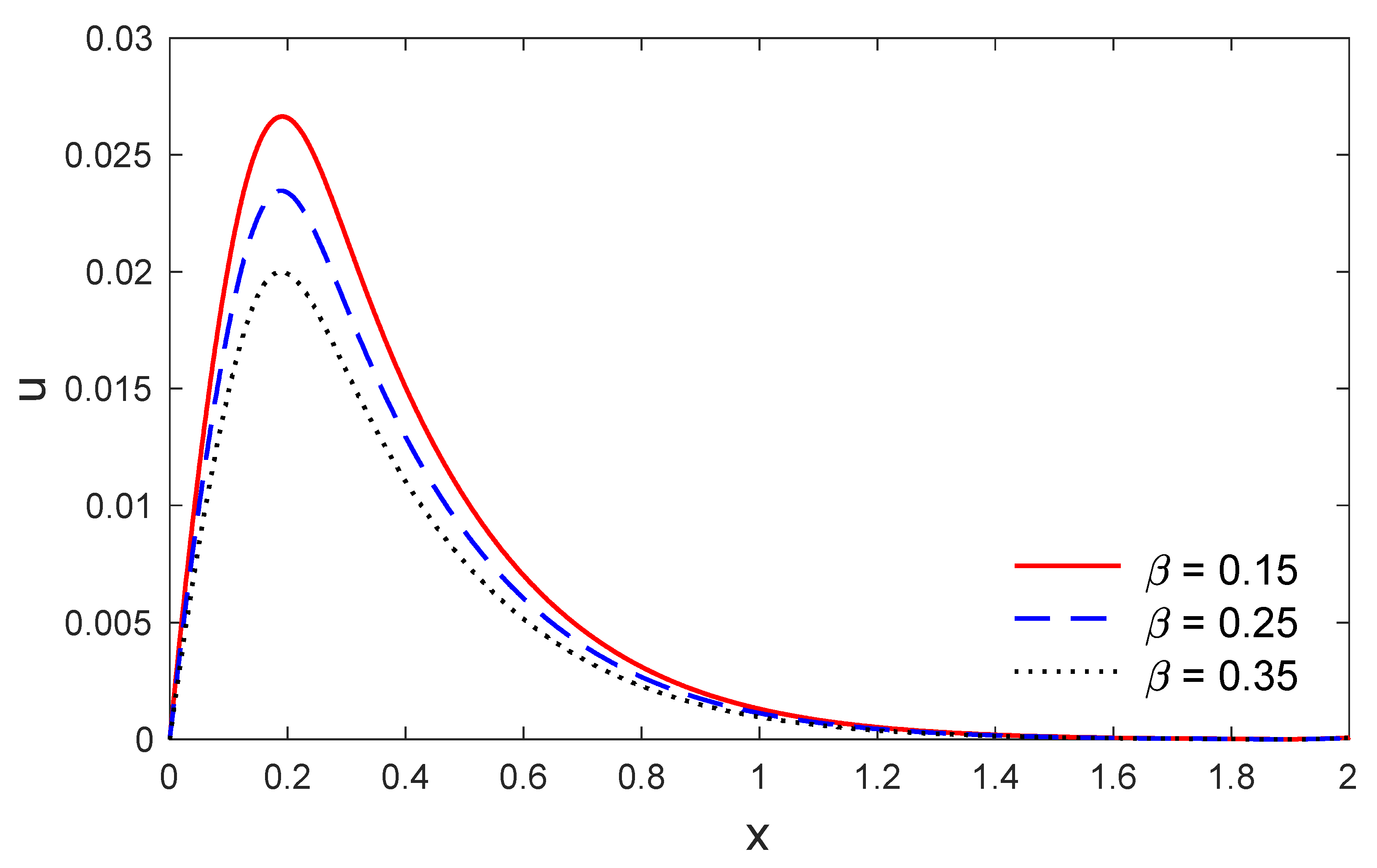
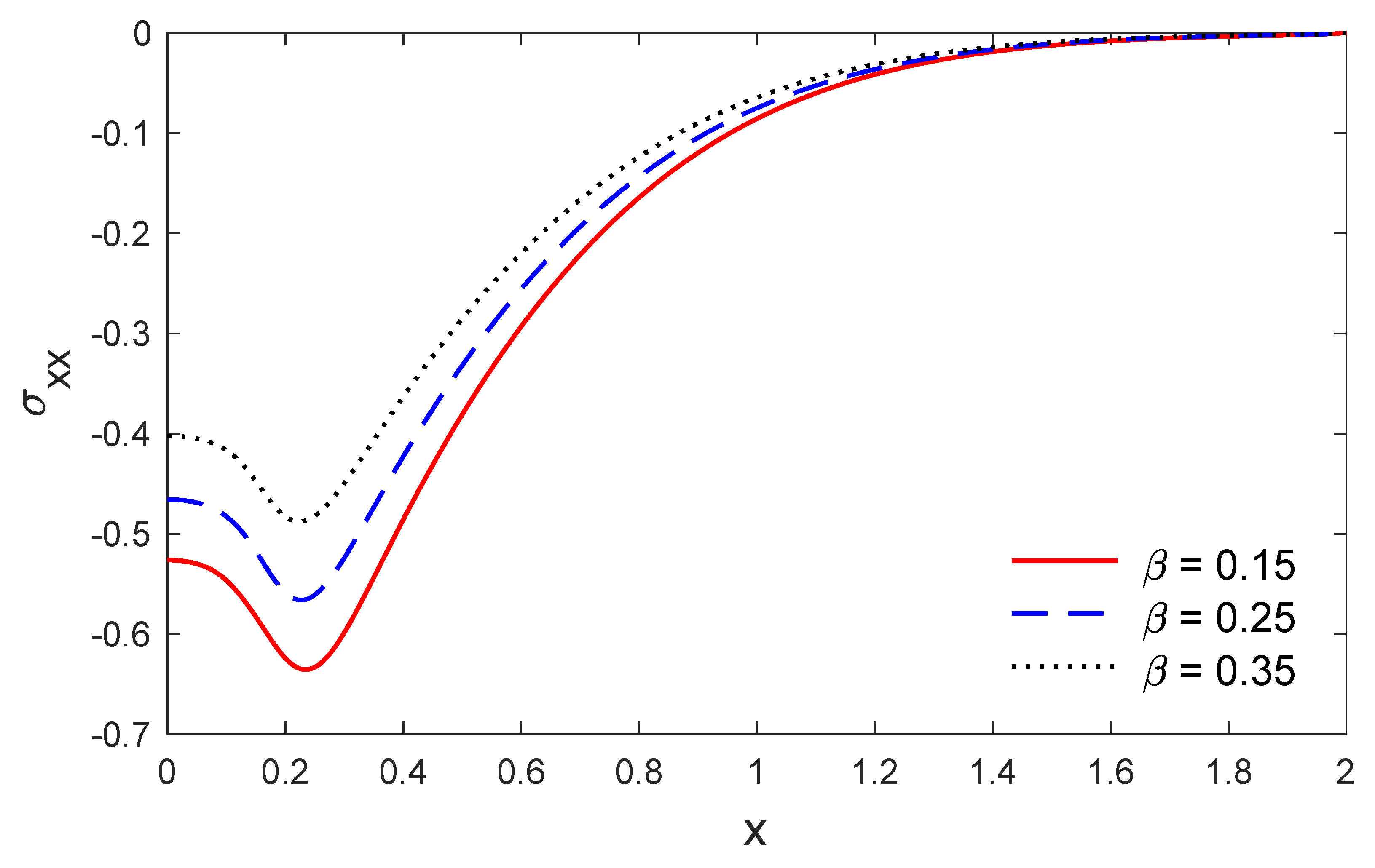
On the basis of the above dataset, Figure 1, Figure 2, Figure 3, Figure 4, Figure 5 and Figure 6 explain the physical quantities calculated numerically versus the distance for several values of porosity. Numerical calculations are carried out for the fluid and solid displacements, solid and fluid temperatures, and the stresses variations of fluid and solid phases versus in the contexts of poro-thermoelastic model with and without energy dispassion. The grid size has been refined until the values of considered fields stabilize. Further refinement of mesh size over 15,000 elements does not change the values considerably. Thus, the grid size 15,000 has been used for this study. Figure 1, Figure 2, Figure 3, Figure 4, Figure 5 and Figure 6 represent the three curves demonstrated by different values of porosity considering . Figure 1 shows the variation of the fluid temperature as a function of . It is observed that the fluid temperature, , has a maximum value for and reduces with an increasing distance to come to zeros at which is according to the value of porosity. Figure 2 demonstrates the variation of the solid temperature along the distance . It is noticed that the solid temperature begins with its maximum value at and gradually reduces with the increasing of until zero beyond the waves front for the porothermoelastic model, which satisfies the boundary conditions of the problem. Figure 3 shows the variations of fluid displacement versus the distance . It is clear that the displacement of fluid started from zero which satisfied the boundary conditions of the problem, and then increases until a maximum value at a particular location near the surface. The variations of solid displacement through the distance are shown in Figure 4. It is clear that the solid displacement begins from zero which satisfied the boundary conditions of the problem, and then it rises up to a maximum value at a specific location within easy reach the surface. Figure 5 and Figure 6 show the effect of the porosity in the fluid and solid stresses versus the distance. As expected, it clear that porosity has a significant effect on the values of all physical quantities.
6. Conclusions
In the present work, the wave propagations in poroelastic material have been studied under generalized poro-thermoelastic theory with and without energy dissipation. The numerical solutions have been obtained using the finite element method and applied to a certain poroelastic material which is thermally shocked on the surface. The effects of porosity are discussed for all physical quantities. The theoretical outcomes can be used as confirmation parts to investigate the practical procedures such as implementation in soil media and rock saturated by groundwaters.
Funding
This project was funded by the Deanship of Scientific Research (DSR) at King Abdulaziz University, Jeddah, Saudi Arabia, under grant no. (KEP-67-130-38). The authors, therefore, acknowledge with thanks DSR technical and financial support.
Conflicts of Interest
The authors declare no conflicts of interest.
References
- Biot, M.A. General solutions of the equations of elasticity and consolidation for a porous material. J. Appl. Mech. 1956, 23, 91–96. [Google Scholar]
- Biot, M.A. Theory of propagation of elastic waves in a fluid-saturated porous solid. II. Higher frequency range. J. Acoust. Soc. Am. 1956, 28, 179–191. [Google Scholar] [CrossRef]
- Biot, M.A. Thermoelasticity and irreversible thermodynamics. J. Appl. Phys. 1956, 27, 240–253. [Google Scholar] [CrossRef]
- Lord, H.W.; Shulman, Y. A generalized dynamical theory of thermoelasticity. J. Mech. Phy. Solids 1967, 15, 299–309. [Google Scholar] [CrossRef]
- Green, A.E.; Naghdi, P.M. Thermoelasticity without energy dissipation. J. Elast. 1993, 31, 189–208. [Google Scholar] [CrossRef]
- Green, A.; Naghdi, P. A re-examination of the basic postulates of thermomechanics. Proc. R. Soc. Lond. Ser. A Math. Phys. Sci. 1991, 432, 171–194. [Google Scholar]
- Schanz, M.; Cheng, A.-D. Transient wave propagation in a one-dimensional poroelastic column. Acta Mech. 2000, 145, 1–18. [Google Scholar] [CrossRef]
- Abbas, I. Natural frequencies of a poroelastic hollow cylinder. Acta Mech. 2006, 186, 229–237. [Google Scholar] [CrossRef]
- Youssef, H. Theory of generalized porothermoelasticity. Int. J. Rock Mech. Min. Sci. 2007, 44, 222–227. [Google Scholar] [CrossRef]
- McTigue, D. Thermoelastic response of fluid-saturated porous rock. J. Geophys. Res. Solid Earth 1986, 91, 9533–9542. [Google Scholar] [CrossRef]
- Singh, B. On propagation of plane waves in generalized porothermoelasticity. Bull. Seismol. Soc. Am. 2011, 101, 756–762. [Google Scholar] [CrossRef]
- Singh, B. Rayleigh surface wave in a porothermoelastic solid half-space. In Proceedings of the Poromechanics VI, Paris, France, 9–13 July 2017; pp. 1706–1713. [Google Scholar]
- Hussein, E.M. Effect of the porosity on a porous plate saturated with a liquid and subjected to a sudden change in temperature. Acta Mech. 2018, 229, 2431–2444. [Google Scholar] [CrossRef]
- El-Naggar, A.; Kishka, Z.; Abd-Alla, A.; Abbas, I.; Abo-Dahab, S.; Elsagheer, M. On the initial stress, magnetic field, voids and rotation effects on plane waves in generalized thermoelasticity. J. Comput. Theor. Nanosci. 2013, 10, 1408–1417. [Google Scholar] [CrossRef]
- Abbas, I.A.; El-Amin, M.; Salama, A. Effect of thermal dispersion on free convection in a fluid saturated porous medium. Int. J. Heat Fluid Flow 2009, 30, 229–236. [Google Scholar] [CrossRef]
- Marin, M.; Öchsner, A. The effect of a dipolar structure on the Hölder stability in Green-Naghdi thermoelasticity. Contin. Mech. Thermodyn. 2017, 29, 1365–1374. [Google Scholar] [CrossRef]
- Abbas, I.A. Nonlinear transient thermal stress analysis of thick-walled FGM cylinder with temperature-dependent material properties. Meccanica 2014, 49, 1697–1708. [Google Scholar] [CrossRef]
- Abbas, I.A.; Abo-Dahab, S. On the numerical solution of thermal shock problem for generalized magneto-thermoelasticity for an infinitely long annular cylinder with variable thermal conductivity. J. Comput. Theor. Nanosci. 2014, 11, 607–618. [Google Scholar] [CrossRef]
- Kumar, R.; Abbas, I.A. Deformation due to thermal source in micropolar thermoelastic media with thermal and conductive temperatures. J. Comput. Theor. Nanosci. 2013, 10, 2241–2247. [Google Scholar] [CrossRef]
- Abbas, I.A.; Zenkour, A.M. LS model on electro-magneto-thermoelastic response of an infinite functionally graded cylinder. Compos. Struct. 2013, 96, 89–96. [Google Scholar] [CrossRef]
- Abbas, I.A.; Youssef, H.M. A nonlinear generalized thermoelasticity model of temperature-dependent materials using finite element method. Int. J. Thermophys. 2012, 33, 1302–1313. [Google Scholar] [CrossRef]
- Abbas, I.A.; Othman, M.I. Generalized thermoelastic interaction in a fiber-reinforced anisotropic half-space under hydrostatic initial stress. J. Vib. Control 2012, 18, 175–182. [Google Scholar] [CrossRef]
- Riaz, A.; Ellahi, R.; Bhatti, M.M.; Marin, M. Study of heat and mass transfer in the Eyring-Powell model of fluid propagating peristaltically through a rectangular compliant channel. Heat Transfer Res. 2019, 50, 1539–1560. [Google Scholar] [CrossRef]
- Sur, A.; Kanoria, M. Memory response on thermal wave propagation in an elastic solid with voids. Mech. Based Des. Struct. Mach. 2020, 48, 326–347. [Google Scholar] [CrossRef]
- Abbas, I.A. Three-phase lag model on thermoelastic interaction in an unbounded fiber-reinforced anisotropic medium with a cylindrical cavity. J. Comput. Theor. Nanosci. 2014, 11, 987–992. [Google Scholar] [CrossRef]
- Sarkar, N.; Mondal, S. Transient responses in a two-temperature thermoelastic infinite medium having cylindrical cavity due to moving heat source with memory-dependent derivative. ZAMM-J. Appl. Math. Mech./Zeitschrift für Angewandte Mathematik und Mechanik 2019, 99, e201800343. [Google Scholar] [CrossRef]
- Othman, M.I.; Mondal, S. Memory-dependent derivative effect on wave propagation of micropolar thermoelastic medium under pulsed laser heating with three theories. Int. J. Numer. Methods Heat Fluid Flow 2019, 30, 1025–1046. [Google Scholar] [CrossRef]
- Abbas, I.A.; Youssef, H.M. Finite element analysis of two-temperature generalized magneto-thermoelasticity. Arch. Appl. Mech. 2009, 79, 917–925. [Google Scholar] [CrossRef]
- Othman, M.I.; Abbas, I.A. Effect of rotation on plane waves at the free surface of a fibre-reinforced thermoelastic half-space using the finite element method. Meccanica 2011, 46, 413–421. [Google Scholar] [CrossRef]
- Sharma, N.; Kumar, R.; Lata, P. Disturbance due to inclined load in transversely isotropic thermoelastic medium with two temperatures and without energy dissipation. Mater. Phys. Mech. 2015, 22, 107–117. [Google Scholar]
- Sur, A.; Kanoria, M. Thermoelastic interaction in a viscoelastic functionally graded half-space under three-phase-lag model. Eur. J. Comput. Mech. 2014, 23, 179–198. [Google Scholar] [CrossRef]
- Zeeshan, A.; Ellahi, R.; Mabood, F.; Hussain, F. Numerical study on bi-phase coupled stress fluid in the presence of Hafnium and metallic nanoparticles over an inclined plane. Int. J. Numer. Methods Heat Fluid Flow 2019, 29, 2854–2869. [Google Scholar] [CrossRef]
- Sheikholeslami, M.; Ellahi, R.; Shafee, A.; Li, Z. Numerical investigation for second law analysis of ferrofluid inside a porous semi annulus: An application of entropy generation and exergy loss. Int. J. Numer. Methods Heat Fluid Flow 2019, 29, 1079–1102. [Google Scholar] [CrossRef]
- Ellahi, R.; Sait, S.M.; Shehzad, N.; Ayaz, Z. A hybrid investigation on numerical and analytical solutions of electro-magnetohydrodynamics flow of nanofluid through porous media with entropy generation. Int. J. Numer. Methods Heat Fluid Flow 2019, 30, 834–854. [Google Scholar] [CrossRef]
- Milani Shirvan, K.; Mamourian, M.; Mirzakhanlari, S.; Rahimi, A.; Ellahi, R. Numerical study of surface radiation and combined natural convection heat transfer in a solar cavity receiver. Int. J. Numer. Methods Heat Fluid Flow 2017, 27, 2385–2399. [Google Scholar] [CrossRef]
- Milani Shirvan, K.; Mamourian, M.; Ellahi, R. Numerical investigation and optimization of mixed convection in ventilated square cavity filled with nanofluid of different inlet and outlet port. Int. J. Numer. Methods Heat Fluid Flow 2017, 27, 2053–2069. [Google Scholar] [CrossRef]
- Marin, M.; Vlase, S.; Ellahi, R.; Bhatti, M. On the partition of energies for the backward in time problem of thermoelastic materials with a dipolar structure. Symmetry 2019, 11, 863. [Google Scholar] [CrossRef] [Green Version]
- Marin, M.; Ellahi, R.; Chirilă, A. On solutions of Saint-Venant’s problem for elastic dipolar bodies with voids. Carpathian J. Math. 2017, 33, 219–232. [Google Scholar]
- Abbas, I.A.; Marin, M. Analytical solution of thermoelastic interaction in a half-space by pulsed laser heating. Phys. E Low-Dimens. Syst. Nanostruct. 2017, 87, 254–260. [Google Scholar] [CrossRef]
- Marin, M.; Nicaise, S. Existence and stability results for thermoelastic dipolar bodies with double porosity. Contin. Mech. Thermodyn. 2016, 28, 1645–1657. [Google Scholar] [CrossRef]
- Marin, M.; Craciun, E.-M.; Pop, N. Considerations on mixed initial-boundary value problems for micropolar porous bodies. Dyn. Syst. Appl. 2016, 25, 175–196. [Google Scholar]
- Ezzat, M.; Ezzat, S. Fractional thermoelasticity applications for porous asphaltic materials. Pet. Sci. 2016, 13, 550–560. [Google Scholar] [CrossRef] [Green Version]
- Abbas, I.A.; Kumar, R. Deformation due to thermal source in micropolar generalized thermoelastic half-space by finite element method. J. Comput. Theor. Nanosci. 2014, 11, 185–190. [Google Scholar] [CrossRef]
- Mohamed, R.; Abbas, I.A.; Abo-Dahab, S. Finite element analysis of hydromagnetic flow and heat transfer of a heat generation fluid over a surface embedded in a non-Darcian porous medium in the presence of chemical reaction. Commun. Nonlinear Sci. Numer. Simul. 2009, 14, 1385–1395. [Google Scholar] [CrossRef]
- Singh, B. Reflection of plane waves from a free surface of a porothermoelastic solid half-space. J. Porous Media 2013, 16, 945–957. [Google Scholar] [CrossRef]
Figure 1.
The variations of fluid temperature with respect to for several values of porosity.

Figure 2.
The variation of solid temperature versus for several values of porosity.

Figure 3.
The variations of fluid displacement versus for several values of porosity.

Figure 4.
The variations of solid displacement with respect to the distance for several values of porosity.
Figure 4.
The variations of solid displacement with respect to the distance for several values of porosity.

Figure 5.
The variations of solid stress versus for several values of porosity.

Figure 6.
The variation of fluid stress versus for several values of porosity.

© 2020 by the author. Licensee MDPI, Basel, Switzerland. This article is an open access article distributed under the terms and conditions of the Creative Commons Attribution (CC BY) license (http://creativecommons.org/licenses/by/4.0/).
Share and Cite
MDPI and ACS Style
Saeed, T. A Study on Thermoelastic Interaction in a Poroelastic Medium with and without Energy Dissipation. Mathematics 2020, 8, 1286. https://doi.org/10.3390/math8081286
AMA Style
Saeed T. A Study on Thermoelastic Interaction in a Poroelastic Medium with and without Energy Dissipation. Mathematics. 2020; 8(8):1286. https://doi.org/10.3390/math8081286
Chicago/Turabian StyleSaeed, Tareq. 2020. "A Study on Thermoelastic Interaction in a Poroelastic Medium with and without Energy Dissipation" Mathematics 8, no. 8: 1286. https://doi.org/10.3390/math8081286
Note that from the first issue of 2016, this journal uses article numbers instead of page numbers. See further details here.