1. Introduction
Image segmentation is a process of partitioning an image into some non-intersecting regions [
1,
2]. Image segmentation is important in many computer vision and image processing applications [
3]. For example, we need to segment MR brain images to get a 3D brain image. Using segmentation technique, we also can detect the head and abdomen of a fetus from an ultrasound image to provide necessary diagnoses and get quantitative estimates of organ sizes [
4]. One of the most widely used methods for binary image segmentation is Chan and Vese model [
5], which is based on the level set method [
6]. In [
7], the authors proposed a completely convex formulation of the algorithm of Chan and Vese when the constant values of each phase are not known a priori. Shi and Pan proposed a local and global binary fitting model using the variational level set approach [
8]. Çataloluk and Çelebi implemented an image segmentation algorithm based Chan–Vese algorithm [
9]. Boykov and Funka-Lea proposed graph cuts based image segmentation [
10]. It uses region-based characteristics using an energy minimization [
11]. Chen et al. [
12] proposed a new diffusion equation model for noisy image segmentation using classical diffusion equation and the segmental process.
The primary purpose of this paper is to present a practical solution algorithm for the previously developed method by the authors in [
13]. In that paper, a multigrid method [
14] was used to solve the equation, which has a limitation in choosing a domain size, i.e., it should be close to square and the grid size should be a power of two for best performance. The essential contribution of this article is to present a computationally simple and efficient explicit hybrid scheme for image segmentation on arbitrary domains.
The contents of this paper are: In
Section 2, the phase-field method for image segmentation is described. In
Section 3, we present the computationally efficient and accurate explicit hybrid scheme. We perform computational tests for image segmentation using the proposed algorithm in
Section 4. The conclusion is made in
Section 5.
2. Phase-Field Model for Image Segmentation
2.1. Mumford–Shah Model
Let
be a bounded image domain. Let
represent a given grayscale image. For the given image
, Mumford and Shah [
15] showed that the image segmentation can be done by the minimization of the functional:
where
u is an approximation to
. Its segmenting curve
C is the edges in
. Parameters
and
are positive constant.
2.2. Chan–Vese Model
Chan and Vese [
5] presented a level set method for the numerical realization of the minimization of the functional (
1). In this approach, the unknown curve
C is the zero level set of continuous function
. Here,
is the signed distance from the interface
C and it satisfies
. Using
, the energy functional is expressed by
here,
is the regularized Heaviside function and
. For example, in the Chan and Vese paper [
5], the regularized Heaviside function is defined as
By applying the gradient descent method, the associated Euler–Lagrange equation is given as
Note that
was used in the original Chan–Vese model.
2.3. Modified Allen–Cahn Model
In the phase-field method, phase function (or order parameter)
is defined by
if
and
if
while it is distributed continuously on thin interfacial layers. A phase-field approximation for minimizing the Chan–Vese functional is given as
here,
and
is a positive parameter. In addition,
and
are the averages of
in the regions which
and
, respectively:
By a variational derivative of energy functional (
2) with respect to
and assuming
and
are constant, we have the following modified Allen–Cahn equation:
For more details about the phase-field model for image segmentation, one may refer to [
13].
3. Numerical Solution Algorithm
In this section, we describe a computationally efficient and accurate explicit hybrid numerical method for the modified AC Equation (
3). For the AC equation part, we use the recently developed explicit hybrid FDM for the AC equation [
16,
17]. By applying the operator splitting scheme, we can split Equation (
3) as a sequence of simpler subproblems:
Let and we discretize the two-dimensional space as the set of cell centers , where and are total number of grid size in x- and y-directions, respectively. Here, is the spatial step size. Let be approximations of , where is the time step size. In the numerical algorithm, we compute the next time step solution with given by going through the following three steps:
- Step (1)
Given a solution
at time
, we solve Equation (
4) analytically and the solution after
is
where
and
are
- Step (2)
Next, we solve Equation (
5) by using the explicit Euler’s method with homogeneous Neumann boundary condition:
- Step (3)
Finally, by using the method of separation of variables [
18,
19], the solution of Equation (
6) is
Here, we note that Equations (
7) and (
9) are unconditionally stable [
13] since the analytic solutions exist for all time steps. However, Equation (
8) has a constraint for stability as
because of the explicit Euler scheme for the heat equation. Therefore, the proposed hybrid scheme is stable if and only if the condition,
, is satisfied. Although the scheme has the restriction for stability, it has the merits of simplicity and versatility for arbitrary computational domains. We define the discrete energy functional as
where
and
.
To help readers understand better, we consider a South Korea license plate image as an example. The numerical algorithm of image segmentation method is described as follows:
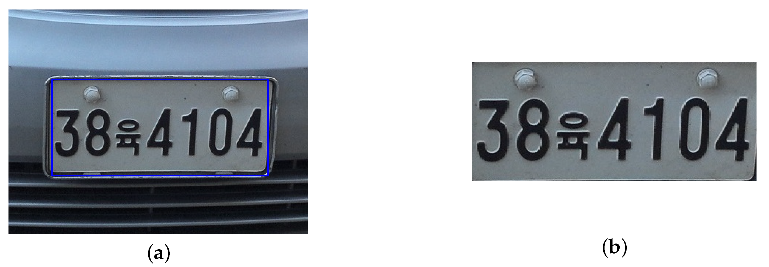
- (i)
Select the real image
f for image segmentation (see
Figure 1a) and change it into a grayscale image as shown in
Figure 1b.
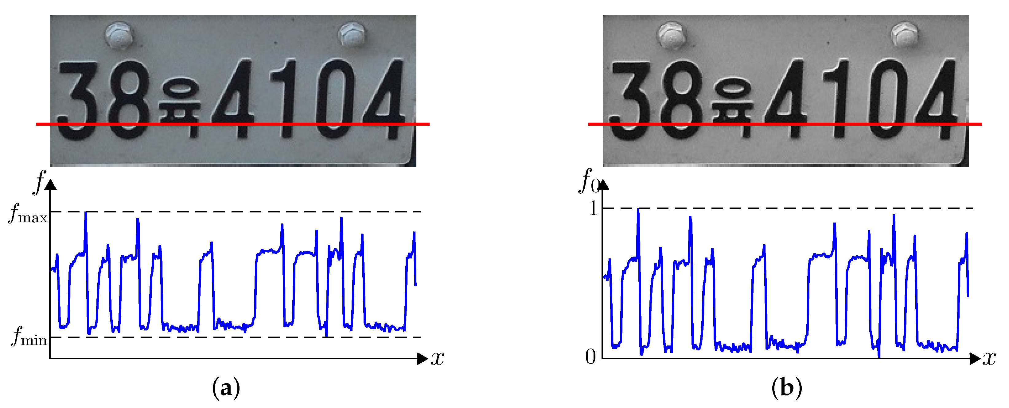
- (ii)
Normalize the given image
f as
where
and
are the maximum and the minimum values of the given image
f, respectively, (see
Figure 2).
- (iii)
Obtain numerical approximation to the given image
by the explicit hybrid scheme, that is described from
Steps (1)–(3). Since solutions with the proposed numerical algorithm are almost insensitive to the initial condition of
, we simply initialize
. We can use the other initial condition. We stop the computation if
. Here, the discrete total energy
is defined by Equation (
2). Refer to Algorithm 1 for the procedure.
| Algorithm 1 Image segmentation. |
Set the initial condition as , N, a tolerance , and .
while do
Compute from by solving Equations (4)–(6).
if then
Stop the calculation.
end if
Set
end while |
4. Numerical Experiments
We perform numerical tests using the proposed method on synthetic and real images. In the AC equation without a fidelity term, across the interfacial regions, varies from to over a distance of approximately . Let , which implies we have approximately m grid points if we use .
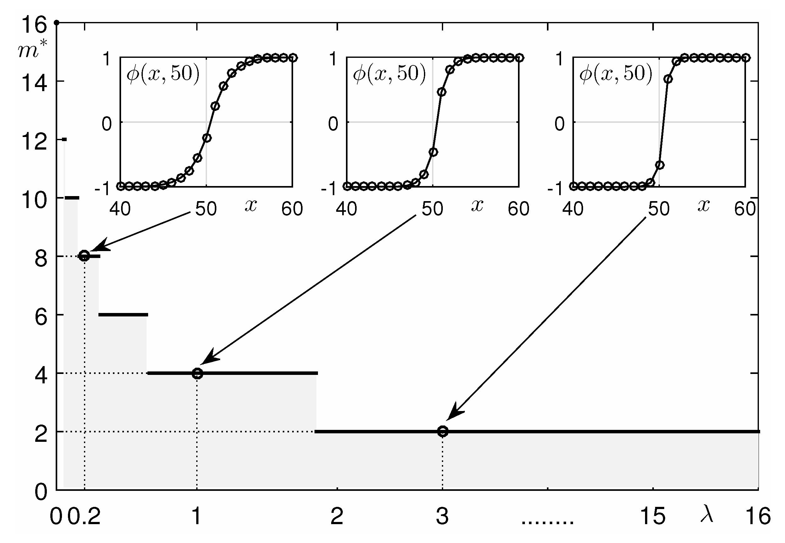
4.1. Effect of
We first consider a given image data:
if
; otherwise
on
To study the effect of
, we perform numerical tests with several
values with
,
,
, and
.
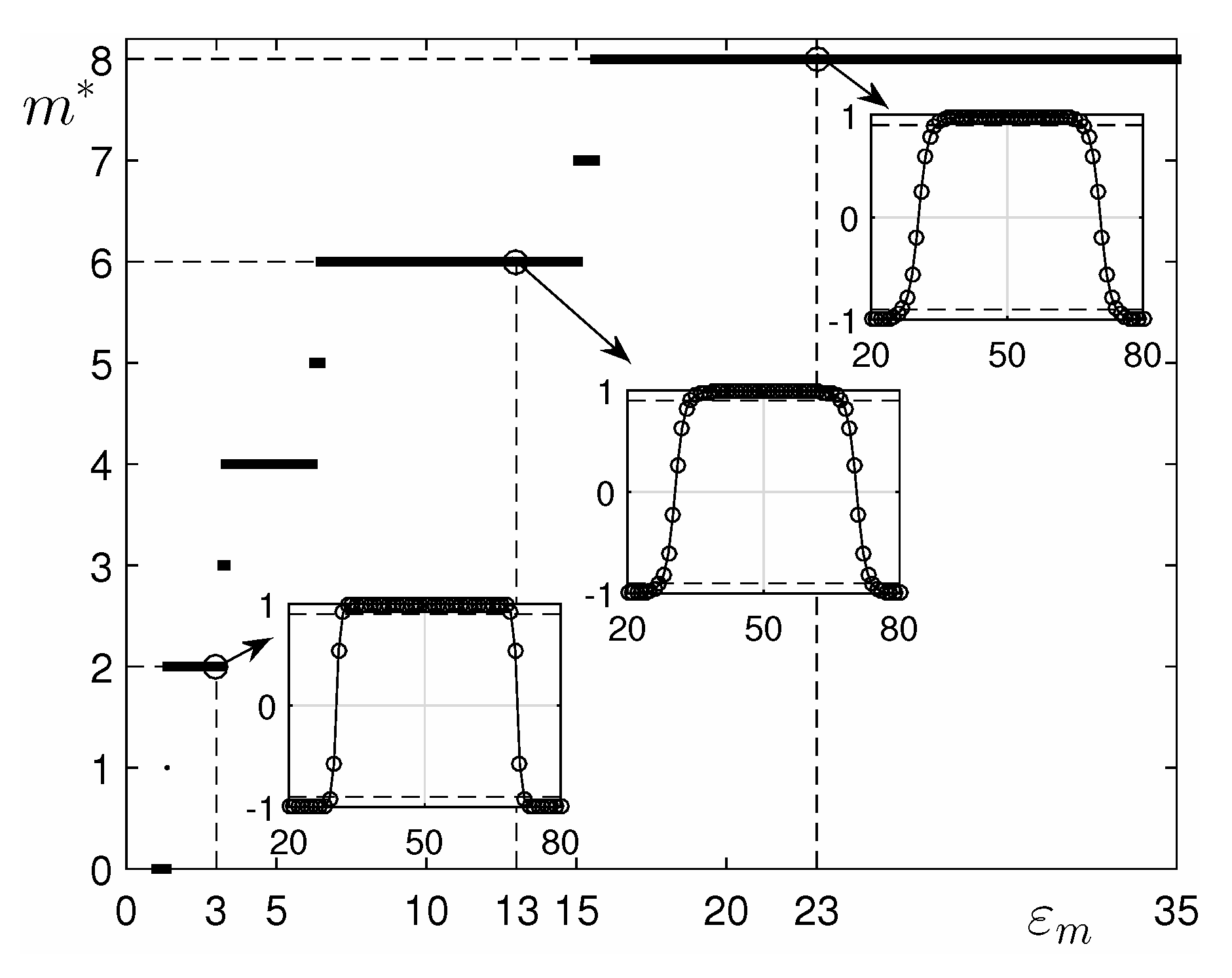
Figure 3 shows the relation between
and interface thickness of numerical results at steady state. Here, the notation
means the number of points between the transition layer
and
. The inserted small figures represent the steady profiles
when
, 1, and 3. As shown in
Figure 3, we see that
decreases as
increases, which is also shown in the inserted small figures.
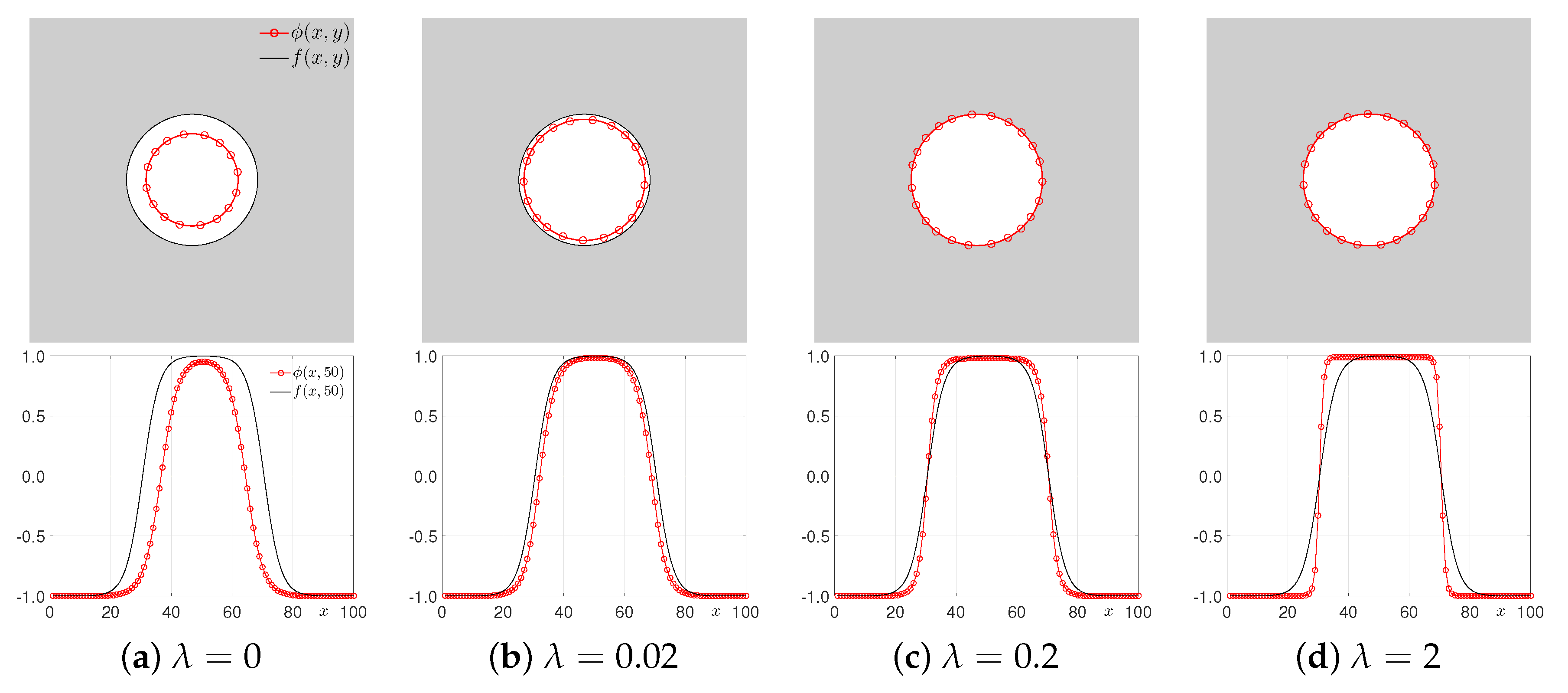
As a second test, we consider the following given image:
We use the initial condition for
as
on the computational domain
and use the following parameters:
,
,
,
, and
.
Figure 4 represents the numerical results at steady state with respect to
. To see the difference, we show the contour image and cross view of the given image
and the numerical solution
. Here, the solid and circle-marked lines are the given image and the numerical solution at steady state, respectively. In this test, we see the standard AC effect when
, i.e., motion by mean curvature. In addition, the numerical solution failed to capture the given image closely when
. From this numerical test, we know that it is important to choose a proper value for
.
4.2. Effect of
Next, we study the effect of
, which means the interface thickness of numerical solution. For this test, the given image and initial condition are Equations (
10) and (
11), respectively. The parameters used are space step size
, time step size
,
,
, and
.
Figure 5 shows that the interfacial transition layer is larger as the value of
is larger.
4.3. Character Image Segmentation
Now, we apply our proposed method to several character image segmentations. As an example, we consider the car license plate image which is given in
Section 3. We use
,
,
, and
.
4.3.1. Car License Plate
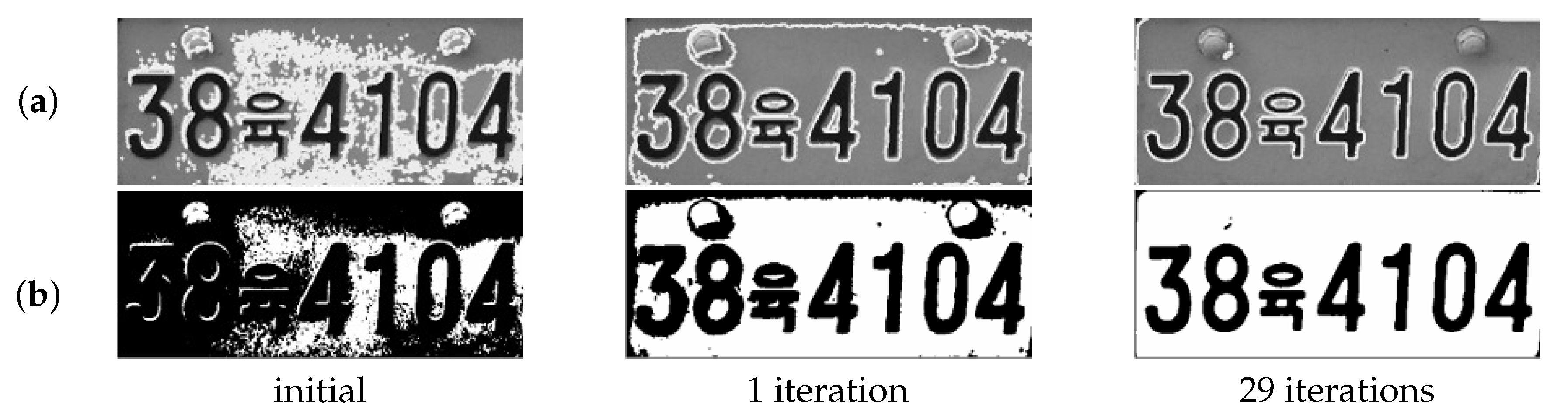
On
, we implement the numerical algorithm with the given image (see
Figure 1b) and
.
Figure 6 shows the temporal evolution of numerical solution. By using our numerical scheme, we obtain the almost segmented image of car license plate in only one iteration and then have final results satisfying the given stop criterion after 29 iterations.
4.3.2. ‘Allen–Cahn Equation’ Text Image
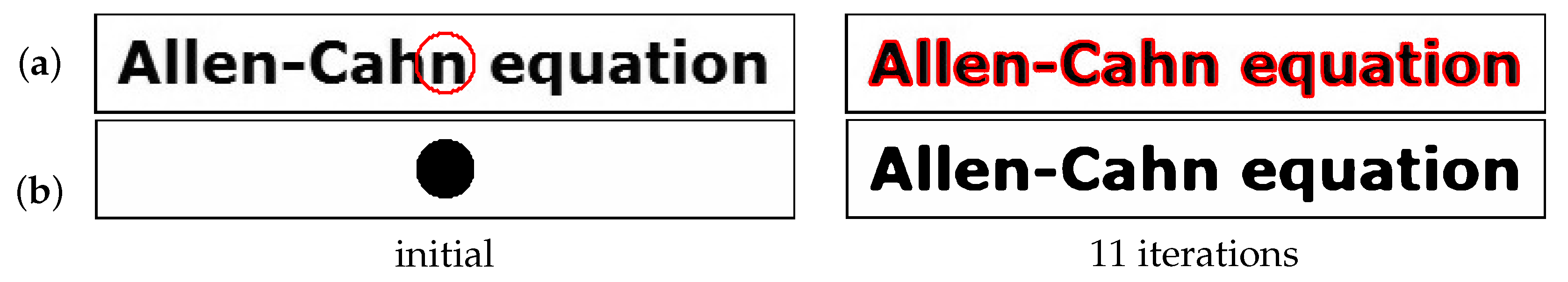
As second test, a character image segmentation is performed for a text image ‘Allen–Cahn equation’ with ‘Vernada’ font on a
mesh with
.
Figure 7 represents Allen–Cahn equation text image and its segmented image. The first and second column is the original images and the segmented image, respectively. We can obtain the good segmented image after 11 iterations. In this test, we set the initial condition with a small circle as
if
; otherwise
.
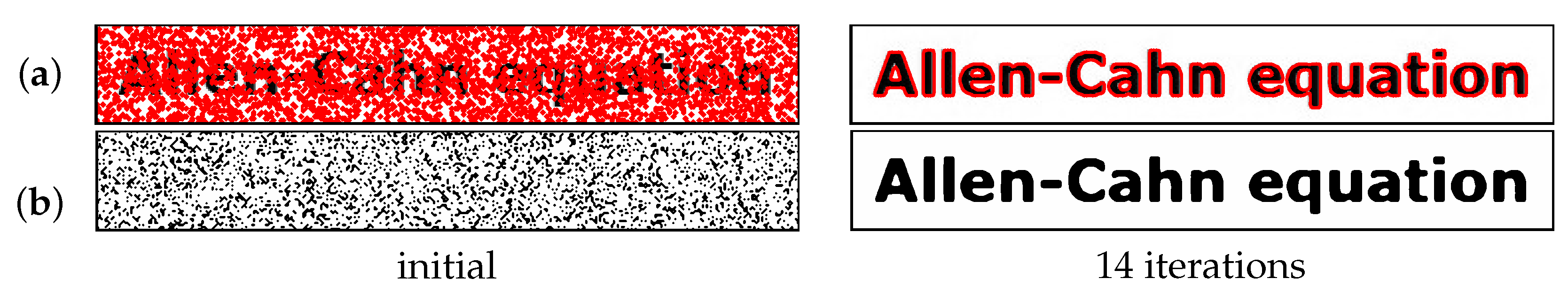
Next, we perform Allen–Cahn equation text image segmentation with random initial condition, that is set with
salt-and-pepper noise.
Figure 8a shows the overlapped original image and zero contour line of
at initial state and after 14 iterations. Additionally, we can see the numerical solution
at each time level in
Figure 8b. From these results, we can see that the proposed method presents a good quality segmented image regardless of an initial state.
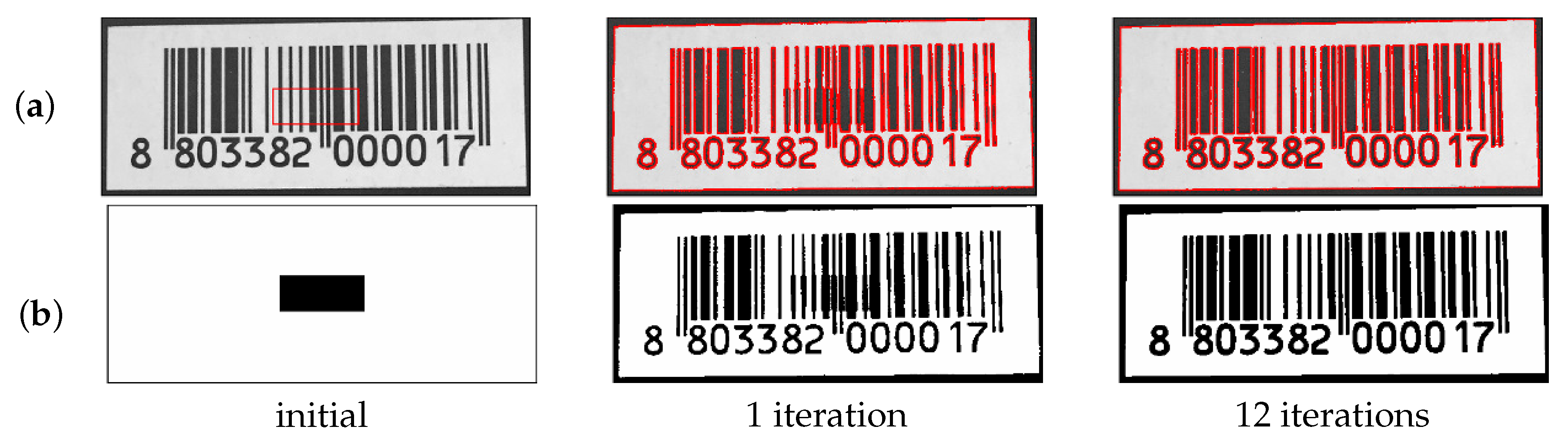
4.3.3. Barcode Image
Now, we consider the barcode image. For this test, we use
on the
mesh. Especially, as shown in first column in
Figure 9, we set the initial condition with a rectangle, that is,
if
and
; otherwise
. In
Figure 9, we can obtain the visually clear results in only one iteration. In addition, we have the final results by the stop criterion after 12 iterations.
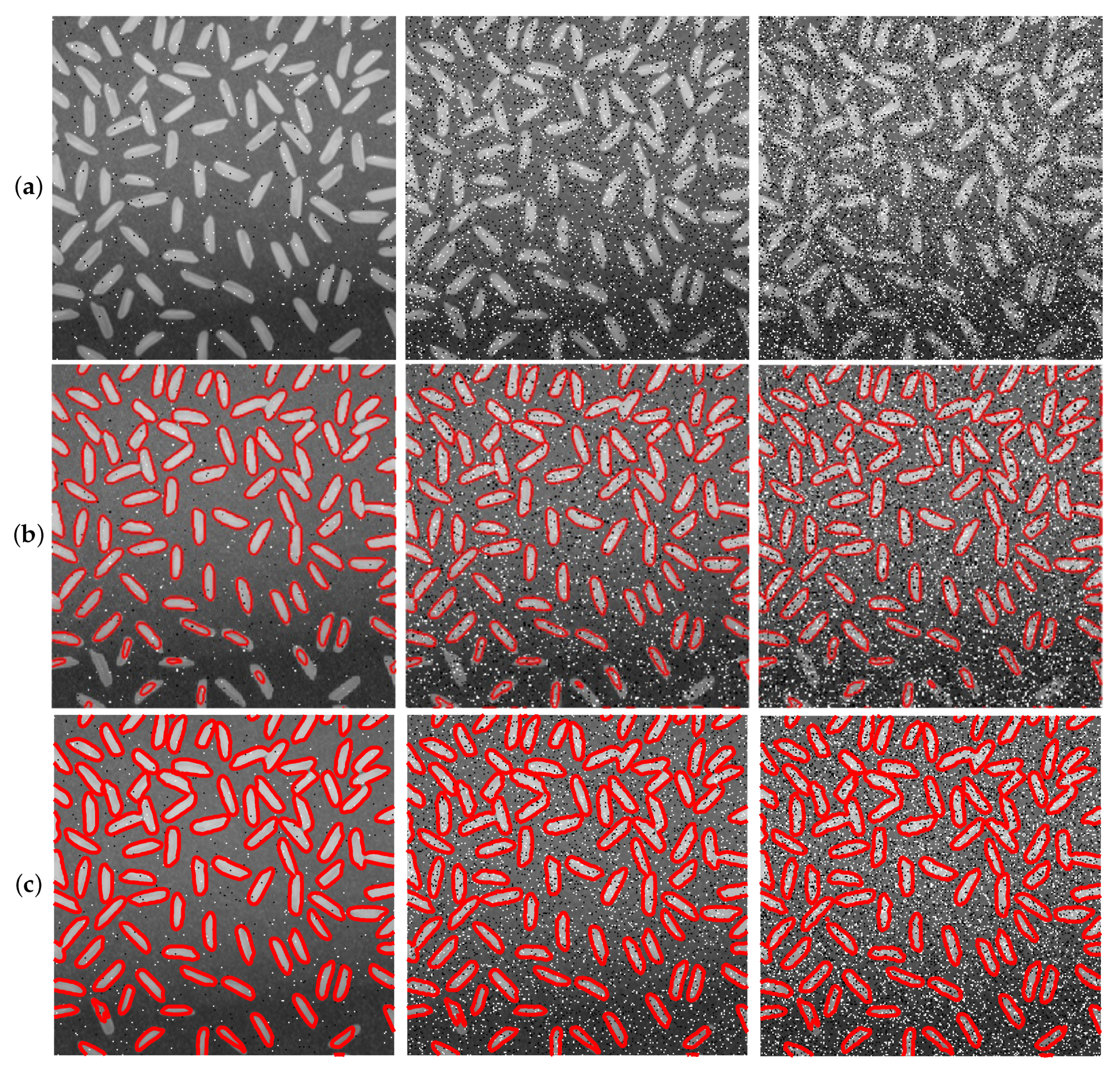
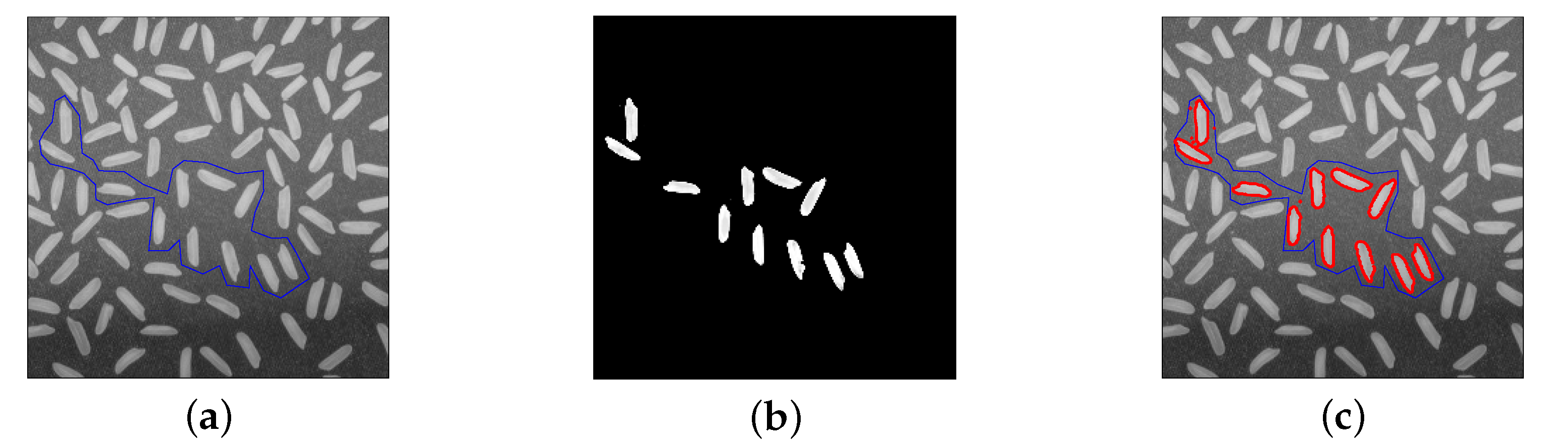
4.3.4. Accuracy of the Proposed Method
In this section, we demonstrate the robustness and accuracy of the proposed method through the given image with salt-and-papers noise. In [
20], a model for image segmentation was proposed by the binary level-set function using
gradient regularizer as regularizing term. For verification, we perform the same experiments which were presented in [
20]. For this test, we use
, and
on a
mesh grid.
Figure 10a shows that the original rice image is degraded by different noise density levels. Here, we use three different levels:
, and
from left to right columns in
Figure 10a.
Figure 10b shows the numerical result by the previous method [
20]. We can observe that the rice grains in bottom region are not well segmented using the previous method. However, the proposed model can segment almost all rice grains as shown in
Figure 10c. In the noisy image, the proposed model has a relatively high accuracy compared to the other model [
20].
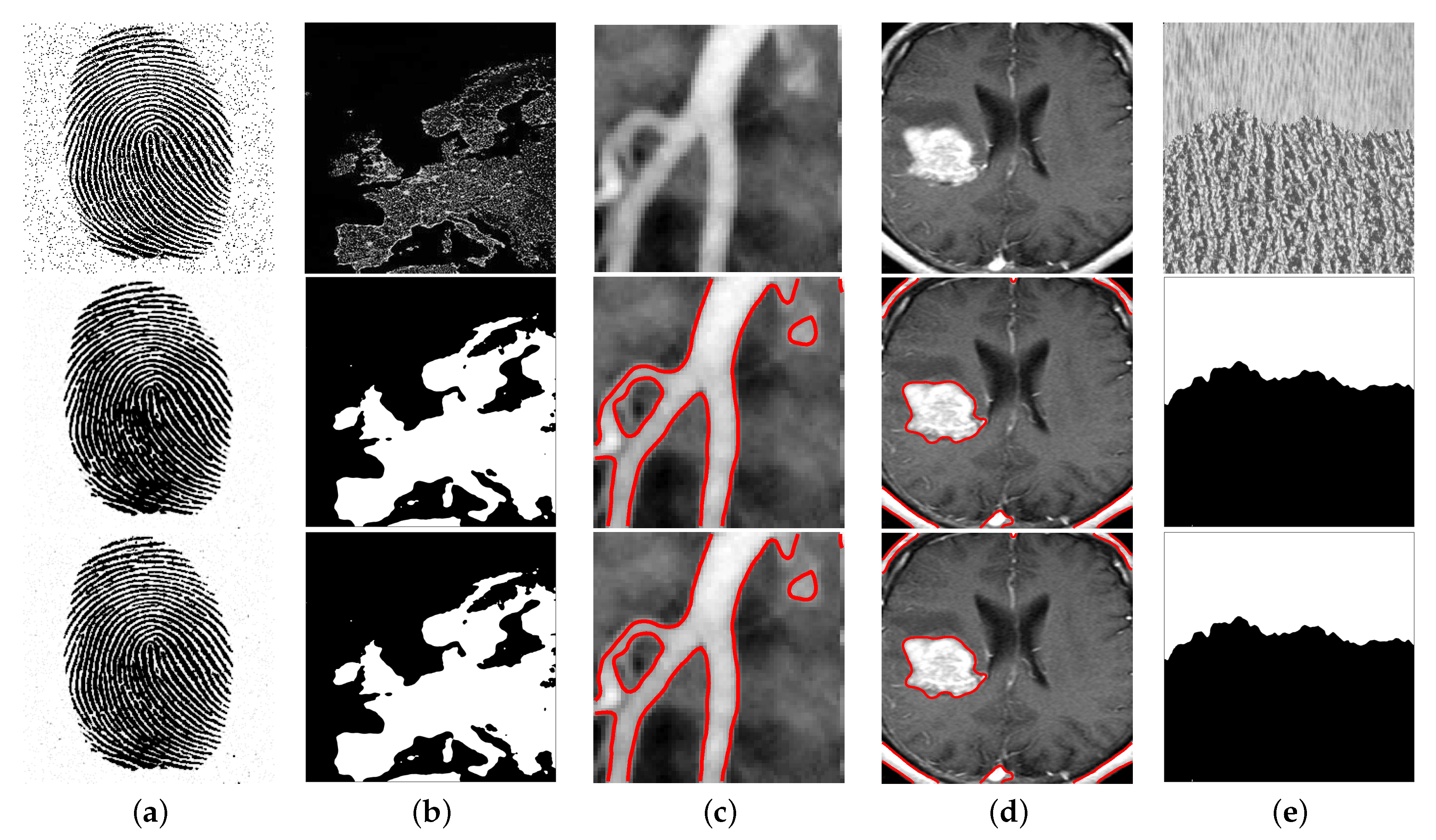
4.4. Comparison with the Previous Method
We demonstrate the performance of the five test problems that are fingerprint, Europe night-lights, blood vessel, brain MRI, and texture images used in [
13] and compare the results between the two methods.
Figure 11 shows the initial image and segmented results of the previous method [
13], and the proposed method. Tests were performed on a 2.70 GHz Intel Core i5-6400 CPU with 4.00 GB of RAM. We used
and
. Other parameters are in
Table 1.
In recent researches, a multigrid method is known as one of the fastest technique in solving the common discretized equation [
14]. Therefore, it is frequently used for image segmentation [
13,
21,
22] since the method can overcome convergence rate degradation and speed up the computation. However, the multigrid method has a restriction in choosing the number of pixels of input image because of its methodology. In this section, we show the advantage of our proposed method by comparing with the previous method [
13].
Figure 12a–c represent the original image, the initial condition, and segmented result with
pixels, respectively. Note that 89 and 97 are the prime numbers which have difficulties in using the multigrid method.
Figure 12d represents the image segmentation using the previous method in [
13], which uses a multigrid method with
pixels. Other parameters are the same as the simulation in the previous section.
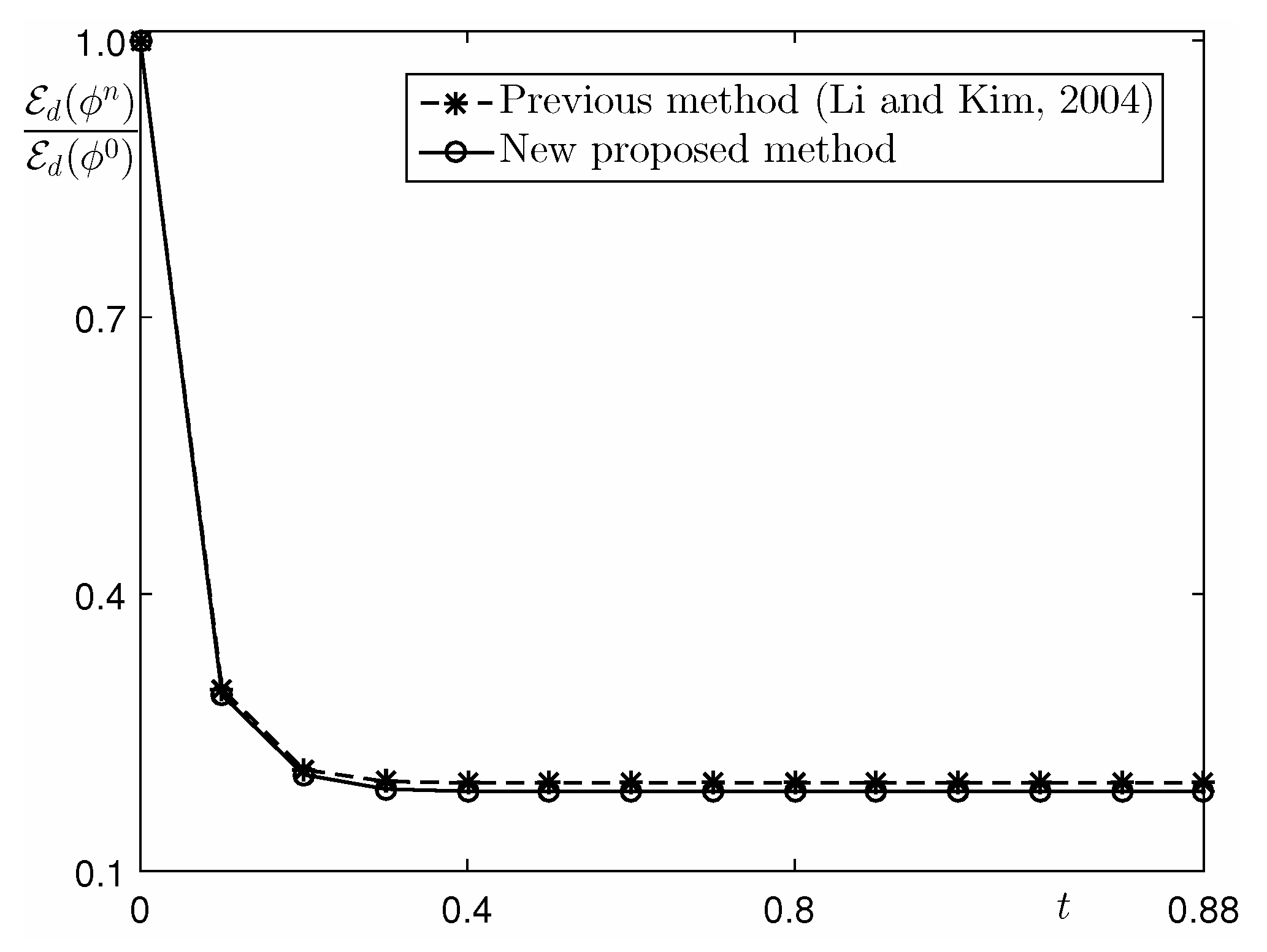
Figure 13 shows the evolutions of normalized total discrete energy
for numerical solution by the previous method [
13] and new proposed method. As we expected, both energies are shown the non-increasing behavior. Especially, the proposed method is slightly lower than the previous method.
Moreover, we can show the time step size
, the number of iterations, and CPU time (s) in
Table 2. Since the previous method in [
13] applies an implicit scheme in solving Equation (
5), a larger time step can be used than the proposed one and it may reduce the number of iterations for image segmentation. Nevertheless, the CPU time is less when our proposed algorithm is applied in spite of same number of iterations. It results from the cheap computational cost of an explicit scheme.
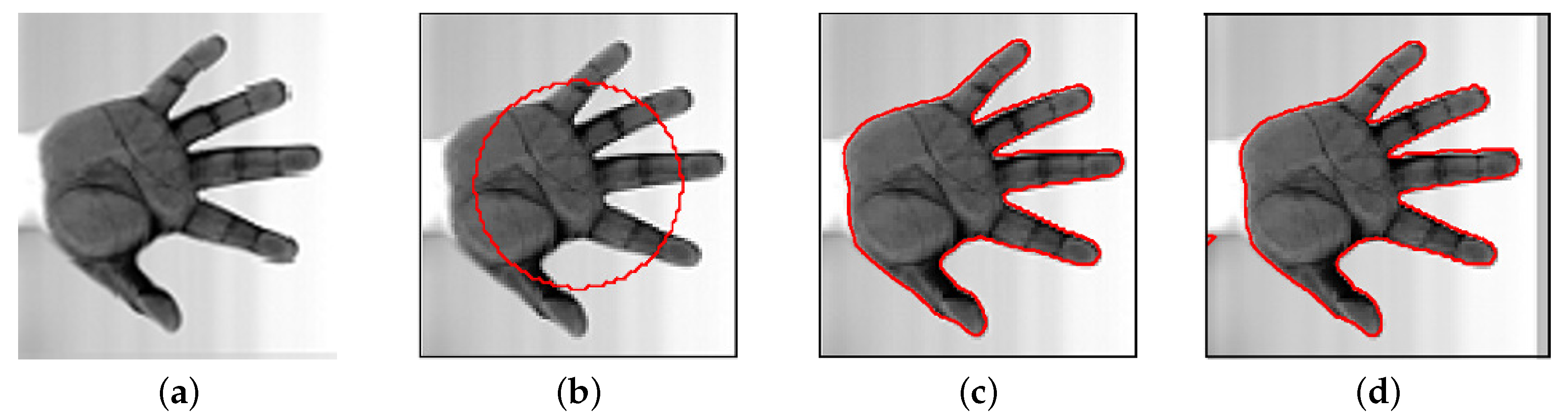
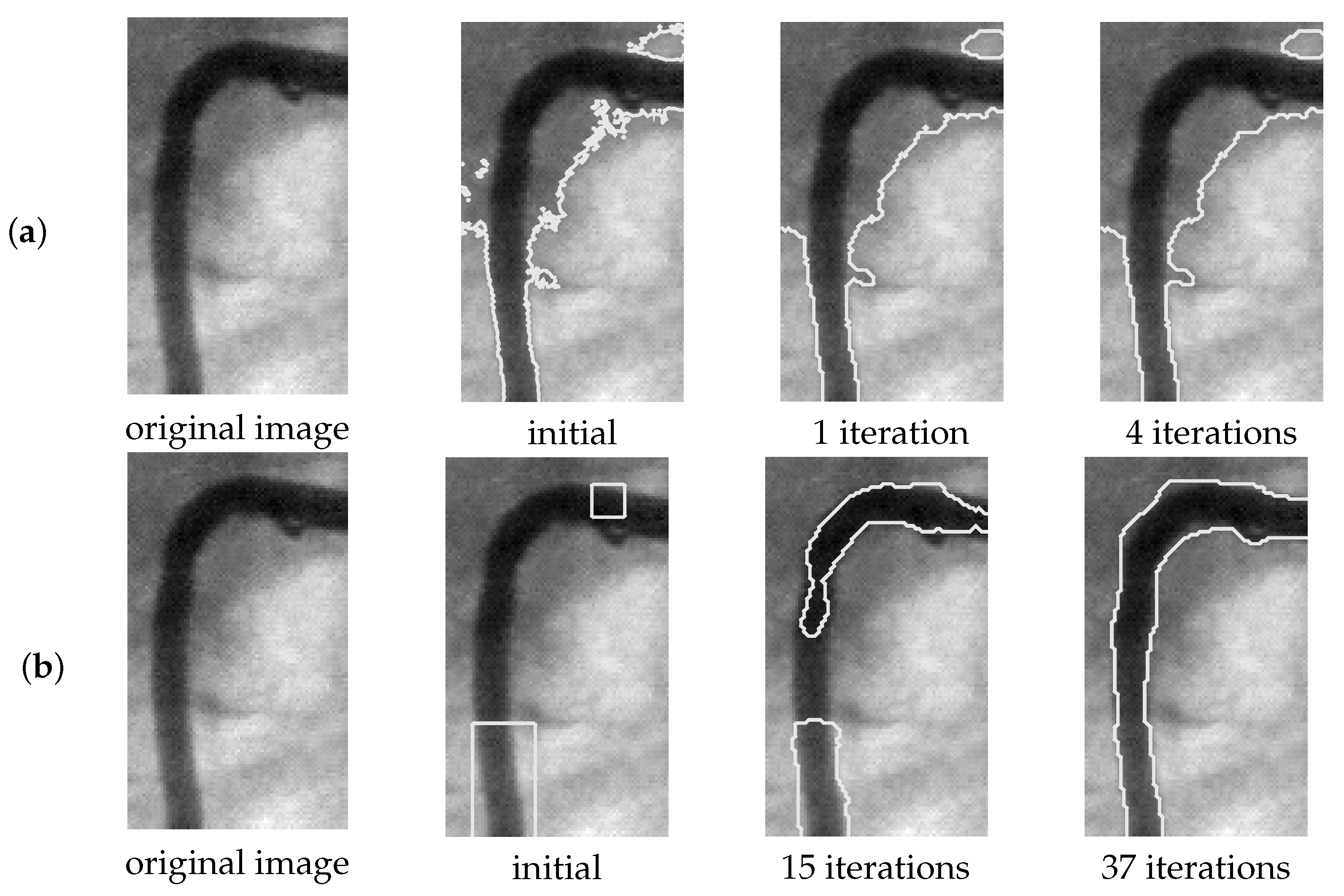
4.5. Application in Medical Image: Coronary Artery
The coronary artery is a vessel that delivers oxygen-rich blood to the myocardium. The effective technique in imaging coronary arteries is important to avoid complicated clinical procedures and risks to the patient [
24]. An image of an artery may have large unnecessary area in square-shaped one because of the artery’s structure and it is inefficient to perform image processing like segmentation.
Figure 14 represents the original coronary artery image from [
25], the initial condition, and segmented results with
pixels. Here, the parameters are used as
and
. As shown in
Figure 14, the original image has inhomogeneous intensity. By this property, segmentation of the original image is sensitive to the initial condition. In this case, the active contour scheme [
5,
26] is more suitable for image segmentation because we can capture the target object with intensity inhomogenity using the active contours and they can handle intensity variations across the regions in the domain. Therefore, it is important to determine the appropriate initial condition for good results. To show this, we implement tests with two different initial conditions;
and two specific rectangles. See second column in
Figure 14. As numerical results, we can see that the test with two specific rectangles has a good segmented image.
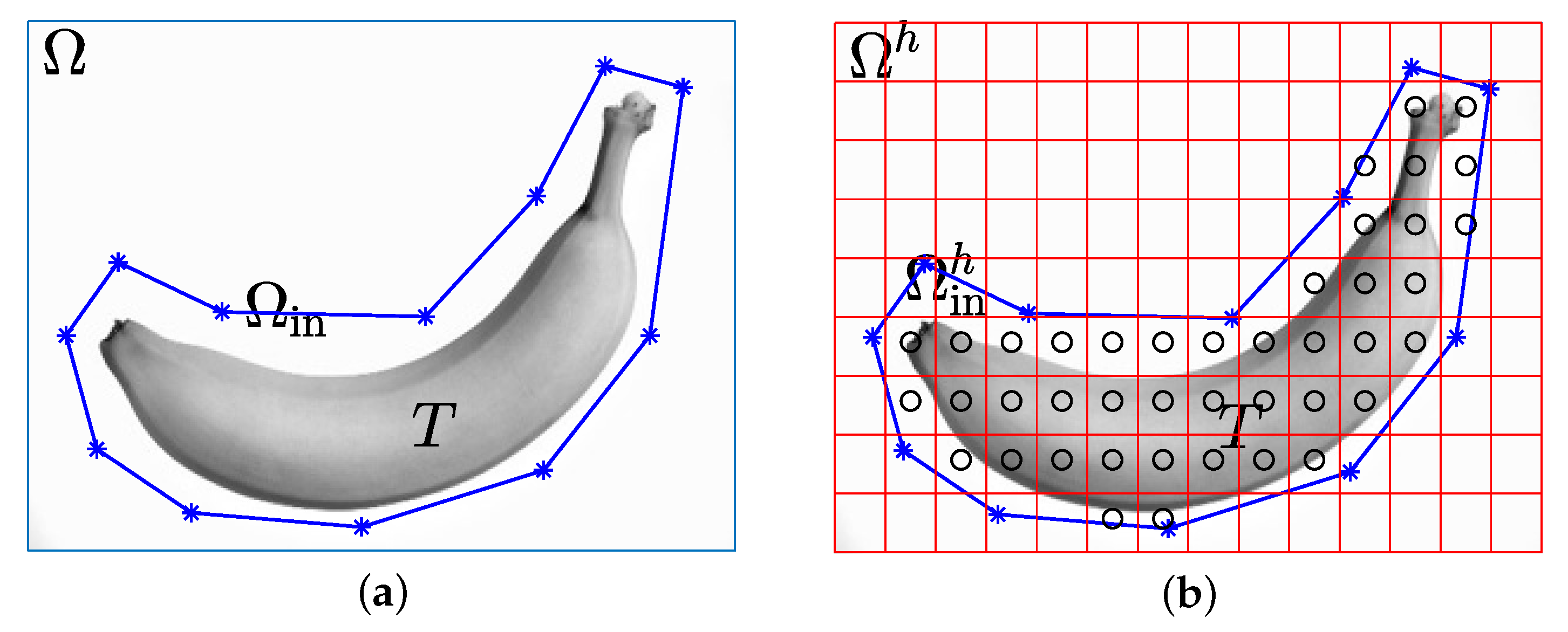
4.6. Image Segmentation on Arbitrary Domain
Our numerical scheme is based on analytic formulae and explicit scheme. Therefore, it has an advantage to obtain the numerical solution which is defined on complex domain. However, the other solver such as multigrid or FFT is not efficient to solve the discrete equation on complex domain. In this section, we introduce a simple algorithm for image segmentation on arbitrary domain.
Let
T be a target image which we want to extract. Let
be an user-selected arbitrary domain which contains the target image
T and is embedded in the whole domain
.
Figure 15a illustrates the target image
T and its user-selected arbitrary domain
. In this figure, we construct the closed domain
with 13 points. Furthermore, let
be a discrete domain,
be its discrete boundary as shown in
Figure 15b with spatial step size
h. Here, the computational domain
is approximated by
as
.
Now, we only proceed the three steps for image segmentation on an arbitrary domain . Note that for efficient calculation, we convert in into a vector form , where .
- Step (1)
Given a solution
at time
, we solve Equation (
4) analytically as follows: For
,
here,
and
.
- Step (2)
Next, we solve Equation (
5) by using the explicit Euler’s method with homogeneous Neumann boundary condition:
- Step (3)
Finally, by using the method of separation of variables, the solution of Equation (
6) is
for
.
As the example, we segment original rice image into a part which we want. For numerical test, we use
and
.
Figure 16a–c show rice image and target domain, segmented image, and segmented contour line with original image, respectively. We can observe the flexibility of the proposed method.
5. Conclusions
In this paper, we presented a computationally fast and accurate explicit hybrid method for image segmentation. By using a gradient flow, the governing equation is derived from a phase-field model to minimize the Chan–Vese functional for image segmentation. The resulting governing equation is the Allen–Cahn equation with a nonlinear fidelity term. The numerical solution algorithm consists of the two closed-form solutions and one explicit Euler’s method. Even though the scheme is explicit, the proposed scheme has the merits of simplicity and versatility for arbitrary computational domains. We presented computational experiments to demonstrate the efficiency of the proposed image segmentation algorithm on real and synthetic images.
Author Contributions
Conceptualization, D.J. and J.K.; Investigation, S.K. and C.L.; Methodology, J.K.; Project administration, D.J. and J.K.; Software, D.J.; Supervision, J.K.; Validation, S.K. and C.L.; Visualization, S.K. and C.L.; Writing original draft, D.J. and J.K.; Writing review and editing, C.L. All authors contributed equally. All authors have read and agreed to the published version of the manuscript.
Funding
The first author (D. Jeong) was supported by the National Research Foundation of Korea (NRF) grant funded by the Korea government (MSIP) (NRF-2017R1E1A1A03070953).
Acknowledgments
The authors greatly appreciate the reviewers for their constructive comments and suggestions, which have improved the quality of this paper.
Conflicts of Interest
The authors declare no conflict of interest.
References
- Pal, N.R.; Pal, S.K. A review on image segmentation techniques. Pattern Recognit. 1993, 26, 1277–1294. [Google Scholar] [CrossRef]
- Zhang, Y.J. Evaluation and comparison of different segmentation algorithms. Pattern Recognit. Lett. 1997, 18, 963–974. [Google Scholar] [CrossRef]
- Umbaugh, S.E.; Moss, R.H.; Stoecker, W.V.; Hance, G.A. Automatic color segmentation algorithms-with application to skin tumor feature identification. IEEE Eng. Med. Biol. Mag. 1993, 12, 75–82. [Google Scholar] [CrossRef]
- Wasilewski, M. Active contours using level sets for medical image segmentation. In Medical Imaging: Segmentation; University of Waterloo: Waterloo, ON, Canada, 2014. [Google Scholar]
- Chan, T.; Vese, L. Active contours without edges. IEEE Trans. Image Process. 2001, 10, 266–277. [Google Scholar] [CrossRef] [PubMed] [Green Version]
- Osher, S.; Sethian, J.A. Fronts propagating with curvature-dependent speed: Algorithms based on Hamilton–Jacobi formulations. J. Comput. Phys. 1988, 79, 12–49. [Google Scholar] [CrossRef] [Green Version]
- Brown, E.S.; Chan, T.F.; Bresson, X. Completely convex formulation of the Chan–Vese image segmentation model. Int. J. Comput. Vis. 20012, 98, 103–121. [Google Scholar] [CrossRef]
- Shi, N.; Pan, J. An improved active contours model for image segmentation by level set method. Optik 2016, 127, 1037–1042. [Google Scholar] [CrossRef]
- Çataloluk, H.; Çelebi, F.V. A novel hybrid model for two-phase image segmentation: GSA based Chan–Vese algorithm. Eng. Appl. Artif. Intell. 2018, 73, 22–30. [Google Scholar] [CrossRef]
- Boykov, Y.; Funka-Lea, G. Graph cuts and efficient N-D image segmentation. Int. J. Comput. Vis. 2006, 70, 109–131. [Google Scholar] [CrossRef] [Green Version]
- Bauer, S.; Wiest, R.; Nolte, L.P.; Reyes, M. A survey of MRI-based medical image analysis for brain tumor studies. Phys. Med. Biol. 2013, 58, R97–R129. [Google Scholar] [CrossRef]
- Chen, B.; Zhou, X.H.; Zhang, L.W.; Wang, J.; Zhang, W.Q.; Zhang, C. A new nonlinear diffusion equation model for noisy image segmentation. Adv. Math. Phys. 2016, 2016, 8745706. [Google Scholar] [CrossRef] [Green Version]
- Li, Y.; Kim, J. An unconditionally stable hybrid method for image segmentation. Appl. Numer. Math. 2014, 82, 32–43. [Google Scholar] [CrossRef]
- Trottenberg, U.; Oosterlee, C.W.; Schüller, A. Multigrid; Academic Press: London, UK, 2001. [Google Scholar]
- Mumford, D.; Shah, J. Optimal approximation by piecewise smooth functions and associated variational problems. Commun. Pure Appl. Math. 1989, 42, 577–685. [Google Scholar] [CrossRef] [Green Version]
- Oyjinda, P.; Pochai, N. Numerical simulation to air pollution emission control near an industrial zone. Adv. Math. Phys. 2017, 2017, 5287132. [Google Scholar] [CrossRef] [Green Version]
- Jeong, D.; Kim, J. An explicit hybrid finite difference scheme for the Allen–Cahn equation. J. Comput. Appl. Math. 2018, 340, 247–255. [Google Scholar] [CrossRef]
- Stuart, A.; Humphries, A.R. Dynamical System and Numerical Analysis; Cambridge University Press: Cambridge, UK, 1998. [Google Scholar]
- Li, Y.; Lee, H.G.; Jeong, D.; Kim, J. An unconditionally stable hybrid numerical method for solving the Allen–Cahn equation. Comput. Math. Appl. 2010, 60, 1591–1606. [Google Scholar] [CrossRef] [Green Version]
- Biswas, S.; Hazra, R. A new binary level set model using L0 regularizer for image segmentation. Signal. Process. 2020, 174, 107603. [Google Scholar] [CrossRef]
- Yang, X.; Gao, X.; Tao, D.; Li, X.; Li, J. An efficient MRF embedded level set method for image segmentation. IEEE Trans. Image Process. 2015, 24, 9–21. [Google Scholar] [CrossRef]
- D’Ambra, P.; Tartaglione, G. Solution of Ambrosio—Tortorelli model for image segmentation by generalized relaxation method. Commun. Nonlinear Sci. Numer. Simul. 2015, 20, 819–831. [Google Scholar] [CrossRef]
- Ramirez-Cortes, J.M.; Gomez-Gil, P.; Sanchez-Perez, G.; Prieto-Castro, C. Shape-based hand recognition approach using the morphological pattern spectrum. J. Electron. Imaging 2009, 18, 013012. [Google Scholar]
- Yang, Y.; Tannenbaum, A.; Giddens, D. Knowledge-based 3D segmentation and reconstruction of coronary arteries using CT images. In Proceedings of the 26th Annual International Conference of the IEEE Engineering in Medicine and Biology Society, San Francisco, CA, USA, 1–5 September 2004; pp. 1664–1666. [Google Scholar]
- Berenguer, A.; Mainar, V.; Bordes, P.; Valencia, J.; Arrarte, V. Spontaneous coronary artery dissection. An infrequent cause of acute coronary syndromes. Rev. Esp. Cardiol. 2003, 56, 1017–1021. [Google Scholar] [CrossRef]
- Dai, L.; Ding, J.; Yang, J. Inhomogeneity-embedded active contour for natural image segmentation. Pattern Recognit. 2015, 48, 2513–2529. [Google Scholar] [CrossRef]
© 2020 by the authors. Licensee MDPI, Basel, Switzerland. This article is an open access article distributed under the terms and conditions of the Creative Commons Attribution (CC BY) license (http://creativecommons.org/licenses/by/4.0/).


