Article

Simulation of Natural Convection in a Concentric Hexagonal Annulus Using the Lattice Boltzmann Method Combined with the Smoothed Profile Method

School of Mechanical & Mechatronics Engineering, Kyungsung University, 309, Suyeong-ro (Daeyeon-dong), Nam-gu, Busan 48434, Korea
Mathematics 2020, 8(6), 1043; https://doi.org/10.3390/math8061043
Submission received: 3 June 2020 / Revised: 22 June 2020 / Accepted: 23 June 2020 / Published: 26 June 2020
(This article belongs to the Special Issue Computational Fluid Dynamics 2020)

Abstract

:
This research work presents results obtained from the simulation of natural convection inside a concentric hexagonal annulus by using the lattice Boltzmann method (LBM). The fluid flow (pressure and velocity fields) inside the annulus is evaluated by LBM and a finite difference method (FDM) is used to get the temperature filed. The isothermal and no-slip boundary conditions (BC) on the hexagonal edges are treated with a smooth profile method (SPM). At first, for validating the present simulation technique, a standard benchmarking problem of natural convection inside a cold square cavity with a hot circular cylinder is simulated. Later, natural convection simulations inside the hexagonal annulus are carried out for different values of the aspect ratio, AR (ratio of the inner and outer hexagon sizes), and the Rayleigh number, Ra. The simulation results are presented in terms of isotherms (temperature contours), streamlines, temperature, and velocity distributions inside the annulus. The results show that the fluid flow intensity and the size and number of vortex pairs formed inside the annulus strongly depend on AR and Ra values. Based on the concentric isotherms and weak fluid flow intensity at the low Ra, it is observed that the heat transfer inside the annulus is dominated by the conduction mode. However, multiple circulation zones and distorted isotherms are observed at the high Ra due to the strong convective flow. To further access the accuracy and robustness of the present scheme, the present simulation results are compared with the results given by the commercial software, ANSYS-Fluent®. For all combinations of AR and Ra values, the simulation results of streamlines and isotherms patterns, and temperature and velocity distributions inside the annulus are in very good agreement with those of the Fluent software.

1. Introduction

Natural convection heat transfer in an annular space between two concentric cylinders (also known as concentric annuli) is one of the most studied problems in the field of heat transfer. This fundamental problem has attracted many researchers because of its significance in many engineering applications such as the design of heat exchanger devices, solar energy collectors, cooling of electric power cables, nuclear and chemical reactors, food processing devices, aircraft cabin insulation, etc. [1,2]. For early research works of theoretical and/or experimental investigations on natural convection in an annular space between cold outer and hot inner cylinders, one can find the literature [1,2,3,4,5,6,7,8]. Studying the behavior of natural convection flow in an annulus with irregular geometries (other than the square or rectangular such as circular, elliptical, triangular, and hexagonal) by using the numerical simulations is highly challenging due to complex irregular boundaries. The irregular boundary problems are generally treated with unstructured (body-fitted) grid methods, also known as conforming-mesh methods, which are very complicated and are computationally intensive. In the past two decades, many researchers have paid attention to develop non-conforming-mesh methods, which use a fixed Cartesian grid to simulate the fluid flow in complex geometries. Some of those numerical methods are immersed boundary method (IBM) [9], distributed Lagrange multiplier method or fictitious domain method [10], and smoothed profile method (SPM) [11,12,13].
In the past three decades, the lattice Boltzmann method (LBM) has evolved as a powerful computational technique for solving fluid flow and heat transfer problems. In LBM, one gets the solution for the particle density distribution functions (PDF) (by solving Boltzmann kinetic equation on a discrete lattice mesh) instead of directly solving the pressure and velocity fields. The macroscopic variables (such as pressure, velocity, and temperature) are obtained by calculating the hydrodynamic moments of PDF [14]. Because of its many advantages [15] compared to the classical Navier–Stokes equations solvers, LBM has been successfully used to simulate various Multiphysics problems such as multiphase flows [15,16,17], magnetohydrodynamic (MHD) flows [18,19], micro- and nano-flows [20,21,22] and fluid-solid interactions [13,23,24,25,26]. LBM has also been successfully implemented to predict the behavior of the fluid flow due to natural convection in complex geometries [27,28,29,30,31,32,33,34,35,36,37]. In the above-mentioned research works on natural convection, the following techniques have been used to handle the no-slip and constant temperature BC on complex irregular surfaces: the bounce back (BB) scheme [27,28,29,30,31,32], IBM [33,34,35], and SPM [36,37].
BB rule was first proposed by the Ladd [38,39] to impose the no-slip BC at curved surfaces of solid particles. In this scheme, the irregular surface of a solid body is imagined as a flat edge that lies in-between two neighboring solid and fluid grid points. The no-slip BC can then be achieved with the help of the standard mid-plane BB scheme which bounces back the missing distribution functions coming from the solid nodes to the fluid nodes. Later, Bouzidi et al. [40] and Yu et al. [41] developed an improved version of the Ladd scheme, known as the interpolated bounce back (IBB) scheme to achieve the second-order accuracy for the fluid velocity and temperature. Sheikholeslami et al. [27,28] investigated MHD flow and heat transfer in an annular space between a heated inner circular and a cold outer square cylinder and they reported the fluid flow and heat transfer results at various Ra and AR values. Lin et al. [29] performed simulation of natural convection flow in an annulus between a heated inner circular cylinder, which is located eccentrically, and a cold square enclosure. Bararnia et al. [30] simulated the natural convection between a heated inner elliptical cylinder and a square outer cylinder. They reported the fluid flow and heat transfer characteristics for various combinations of the vertical positions of the inner cylinder and Ra. Sheikholeslami et al. [31] studied the effect of a magnetic field on the fluid flow and heat transfer characteristics of a nanofluid inside a circular cylinder with an inner triangular cylinder. Moutaouakil et al. [32] conducted lattice Boltzmann simulations of natural convection in an annulus between an inner hexagonal cylinder and an outer square cavity. In all the above-mentioned articles [27,28,29,30,31,32], IBB scheme was used to treat the complex boundaries of circular, triangular, elliptical, and hexagonal geometries. Even though IBB scheme can effectively be used for treating the complex curved boundary problems, the main drawback is that there may be fluctuations in the velocity and temperature fields at fluid-solid interfaces especially when the solid boundary is moving with a certain velocity.
In IBM, the complex irregular boundaries of solid bodies are represented with a set of Lagrangian nodes while the evaluation of the fluid flow is considered on a fixed Eulerian grid. To enforce the no-slip and constant temperature BC on the solid nodes, artificial body force and heat source terms are added to fluid momentum and energy equations, respectively. On can refer to the review article by Mittal and Iaccarino [42] for a clear discussion on different approaches for calculating the body force terms. Hu et al. [33] simulated natural convection in a concentric annulus of circular cylinders using LBM and they used IBM to treat the no-slip and isothermal BC on the curved boundaries. Hu et al. [34] developed an immersed boundary lattice Boltzmann method (IBLBM) for simulating fluid flow due to natural convection in a cold square cavity with a heated inner circular cylinder covered by a porous layer. They investigated the effects of thermal conductivity ratio, Ra, and Darcy number on the behavior of fluid flow and heat transfer. Khazaeli et al. [35] used IBLBM to simulate the natural convection due to a hot circular cylinder inside a square and circular enclosures (cold) for different Ra values. IBM could resolve the problem of fluctuations in the velocity field of IBB scheme. However, the main disadvantage of IBM is that it requires complex interpolation functions, and needs a lot of data exchange between the fluid (Eulerian) and solid (Lagrangian) nodes. Therefore, the parallel computational performance of the scheme based on the LBM and IBM becomes lower as the global data communication between the neighboring grid points increases [13].
In SPM, a smoothed profile function is used to recognize the complex surfaces of a solid body, and the same grid system is used for fluid and solid. The no-slip and isothermal BC at the complex surfaces are implemented by adding a hydrodynamic force and heat source terms to the fluid momentum and energy equations, respectively. The main advantage of SPM over the other non-conforming-mesh methods is that all operations are completely local to a grid point as both fluid and solid are represented with the same grid system; so, the implementation of this scheme to parallel computing applications is easier [13]. Also, SPM does not need any complex interpolation function as needed by IBM. Although SPM is computationally more efficient and easier to apply than IBB and IBM schemes, till now, only a few researchers have used the method based on LBM and SPM to study the fluid flow and heat transfer behavior in complex boundaries. Hu et al. [36] used the LBM combined with SPM for simulating natural convection in complex irregular geometries. They reported the simulation results for the velocity and temperature inside a square enclosure with a hot circular cylinder for different values of Ra and AR. All the above-mentioned research works [27,28,29,30,31,32,33,34,35,36] considered the double populations model (DPM) (where two sets of PDF are used: one set for solving the velocity field and another one for the temperature field). Recently, Alapati et al. [37] developed a numerical technique based on the combination of LBM and SPM to simulate particulate flows with heat transfer. They used a hybrid method (HM), which solves the fluid flow by LBM with a set of PDF and the temperature field by FDM and concluded that LBM-SPM method based on HM is computationally more efficient than the method based on DPM.
Fluid flow and heat transfer thorough or over hexagonal-shaped geometries is a ubiquitous problem in many engineering applications such as solar energy collectors [43,44], nuclear power plants [45], microfluidic heat sinks [46], lamella type compact heat exchangers [47], air-conditioning applications [48], etc. In solar energy collectors, to minimize the radiation and convection losses to the surrounding atmosphere, an array of transparent tubes, arranged in a hexagonal honeycomb pattern, is used in-between the absorbing surface and cover plate. Marshall et al. [43] and Buchberg et al. [44] found that the thermal efficiencies of honeycomb solar collectors were higher compared to the collectors without the honeycomb layer. The fuel rods of a nuclear reactor core are stacked in the form of a hexagonal lattice and are located inside a circular or hexagonal channel to pass a coolant longitudinally over them [45]. In a ministered heat sink used for electronic systems cooling, an array of pin-fins of various cross-sectional shapes are attached to a microchannel wall. Aliabadia et al. [44] found that hydrothermal (hydraulic and thermal) performance was best for the pin-fins with the circular and hexagonal cross-sections. Hexagonal duct shape is a commonly used shape in lamella type compact heat exchangers, which is used in many industries such as pulp and paper, alcohol, petrochemical, and other chemical industries [47]. A desiccant disk used in air-conditioning applications consists of an array of several ducts packed in the form of honeycomb pattern. Zhang [48] found that the heat and mass transfer efficiencies of ducts with hexagonal cross-section were higher compared to circular and rectangular ducts as the hexagonal duct walls are more uniformly placed in the desiccant wheel.
Even though it has great significance and applications only a few researchers have investigated the behavior of natural convection flow in an annulus with a heated hexagonal cylinder. Boyd [3] experimentally investigated natural convection in an annulus with a heated hexagonal inner cylinder and cold outer circular cylinder. Raithby et al. [6] simulated the natural convection in an annulus bounded by a circular cylinder outside and horizontal hexagonal cylinder inside by using an orthogonal curvilinear coordinates system (a body-fitted grid system). Galkape and Asfaw [7] employed a non-orthogonal coordinate system to study the same problem of Raithby et al. [6]. More recently, Moutaouakil et al. [32] studied the natural convection due to a hot hexagonal cylinder inside a square enclosure (cold) with LBM. They presented the fluid flow and heat transfer characteristics for different combinations of AR and Ra by considering two orientations for the hexagonal cylinder. As mentioned earlier, they used DPM with IBB scheme to treat BC on hexagonal surfaces.
The literature review showed that the problem of natural convection in an annulus space between two hexagonal cylinders (concentric with each other) has not been studied. The main objective of this work is to solve the problem of two-dimensional natural convection flow caused by a hot hexagonal cylinder placed concentrically inside a cold hexagonal cylinder. The numerical technique that combines LBM, SPM, and FDM methods is employed because it offers many advantages over the other methods. In the present work, an equation for smoothed profile function that identifies the hexagonal boundaries is proposed. Assessing the accuracy and robustness of the present simulation technique by comparing results given by the present method with ANSYS-Fluent® results is also another purpose of this work. The remainder of this paper is arranged as follows. A brief description of the simulation technique is given in Section 2. A discussion on numerical results is presented in Section 3. At first, the validation results, by applying the present simulation scheme to a standard benchmarking test, are provided. Later, the simulation results of streamlines, isotherms, and temperature and velocity distributions inside the concentric hexagonal annulus are presented. The concluding remarks of the present study are provided in Section 4.

2. Numerical Method

Figure 1 shows the simulation set-up, which consists of an annulus region formed by two concentric horizontal hexagonal cylinders of different sizes, considered in the present work. Simulations are performed inside a square enclosure and 251 × 251 lattice grid points are used to divide the computational domain. The center positions of the two hexagonal cylinders are fixed at the center of the enclosure. L o u t in the figure represents the distance between two opposite sides of the outer hexagonal cylinder (the size of the outer cylinder). Throughout the simulations, L o u t is kept constant at L o u t = 212 and the size for the inner hexagonal cylinder, L i n in Figure 1, is varied based on the aspect ratio, which is defined as: AR = L i n / L o u t . g in the figure denotes the gravitational acceleration constant.
The initial values for the fluid velocity and temperature inside the domain are set to zero. The no-slip and constant temperature BC ( T o = T c 0 ) are applied at the enclosure walls for the flow field and temperature field, respectively, and the standard mid-plane BB scheme is used to treat the no-slip boundary condition. The temperature value for all edges/sides of the outer hexagonal cylinder is kept constant at, T o u t T c = 0 (cold surface), and that for the inner one is fixed at T i n T h = 1 (hot surface). The constant temperature and no-slip BC on all sides of the inner and outer cylinder are treated with SPM. In below, the formulations for LBM for solving the fluid flow field, FDM for solving the temperature field, and SPM for treating BC on hexagonal edges are provided.

2.1. Solving Fluid Flow Using LBM

In this work, as mentioned earlier, LBM is used to obtain the flow field due to natural convection. In LBM, the macroscopic variables such as fluid pressure and the velocity, are computed from the fluid-PDF, f n ( x , t ) , which are evaluated by solving the Boltzmann kinetic equation on a discrete lattice mesh. Here, f n ( x , t ) is the probability of finding a fluid particle at a lattice position, x , and at a time, t , moving with a discrete velocity, c n (the subscript n indicates the PDF number), which is selected in such a way that after time step Δ t , the particle arrives at the n t h neighboring grid point [21]. The single-relaxation-time lattice Boltzmann equation (LBE) with external body force term is given by [37]
f n ( x + c n Δ t , t + Δ t ) = f n ( x , t ) 1 λ ( f n ( x , t ) f n e q ( x , t ) ) + w n Δ t c s 2 ( ( f th ( x , t ) + f fl ( x , t ) ) c n )
where λ is the relaxation time, f n e q ( x , t ) is the equilibrium distribution functions, w n is the weighing function, and c s is the sound speed. f th ( x , t ) and f fl ( x , t ) in Equation (1) represent the buoyancy force and the hydrodynamic force (due to the no-slip BC on the hexagonal surfaces) source terms, respectively. Through the Chapman–Enskog analysis, the above equation recovers the Navier–Stokes equations in the low Mach number limit, | u | / c s 1 [14]. The relation between the fluid kinematic viscosity, ν , and relaxation time, λ , is given by
ν = c s 2 Δ t ( λ 1 2 ) .
To model the buoyancy force, f th ( x , t ) , the Boussinesq approximation is used as follows
f th = ρ 0 β ( T T 0 ) g   j ^ ,
where ρ 0 is the initial value for fluid density, T 0 is the initial fluid temperature, β is the fluid thermal expansion coefficient at T 0 , T is the fluid temperature field, and j ^ is the unit vector in the vertical direction ( y   direction). The hydrodynamic force term, f fl ( x , t ) of Equation (1) is obtained with SPM. After solving for f n ( x , t ) , the fluid density and the velocity fields, ρ ( x , t ) and u ( x , t ) , are obtained from
ρ ( x , t ) = n = 0 b f n , u ( x , t ) = 1 ρ n = 0 b f n c n .

2.2. Solving Temperature Distribution with FDM

The temperature distribution inside the computational domain is obtained by discretizing the energy equation with FDM by using the standard central difference scheme in space and the forward difference scheme in time [37]. After discretization, the equation for finding the temperature value at a grid point in new time level is ( q in the below expression represents the heat source term due to the constant temperature BC on the hexagonal edges)
T i , j new = T i , j old + ( RHS old + q i , j old ) Δ t ,
with
RHS old = 4 α T i , j old + ( α 1 2 u i + 1 , j old ) T i + 1 , j old + ( α + 1 2 u i 1 , j old ) T i 1 , j old + ( α 1 2 v i , j + 1 old ) T i , j + 1 old + ( α + 1 2 v i , j 1 old ) T i , j 1 old
In the above equation, α is the thermal diffusivity, and the subscripts i   &   j represent lattice grid indices in x &   y directions, respectively.

2.3. Evaluation of f fl ( x , t ) and q ( x , t ) with SPM

In SPM, a smoothed profile function (also termed as concentration function or indicator function), ϕ k ( x , t ) , is used to identify the solid regions [13] (here, k is the index value for the hexagonal cylinders; k = 1 for the inner hexagon and k = 2 outer one). The equation for ϕ k ( x , t ) is defined in such a way that ϕ k = 0 in the fluid region, ϕ k = 1 in the solid region, and ϕ k smoothly varies from 0 to 1 at the fluid-solid interface. Here, the following equation is used to evaluate ϕ k ( x , t ) of each hexagon
ϕ k ( x , t ) = f ( d k ( x , t ) ) ,
f ( d k ( x , t ) ) = { 0 r < ξ k / 2 1 2 ( sin ( π d k ( x , t ) ξ k ) + 1 ) | r | < ξ k / 2 1 r > ξ k / 2 ,
where d k ( x , t ) and ξ k are the signed normal distance function to the solid surface (here, edges of two hexagons) and the interface thickness of each hexagon, respectively. Unless otherwise mentioned, throughout this work, the values for the interface thickness for the two hexagons are chosen as, ξ 1 = ξ 2 0.5 . The following equation is used for finding d k ( x , t ) of each hexagon
d k ( x , t ) = max { L x , k 2 , max [ ( | x X c , k | sin ( 30 ° ) + | y Y c , k | cos ( 30 ° ) ) , ( | y Y c , k | L y , k 2 ) ] }
L x , k and L y , k in the above equation are the distance between two corners and two opposite sides of each hexagon, respectively ( L y , 1 = L i n and L y , 2 = L o u t are the sizes of the two hexagons), and X c , k and Y c , k are the center positions of hexagons, in x and y directions, respectively. The smoothly distributed concentration field of two hexagons, ϕ ( x , t ) , is obtained by adding the ϕ k ( x , t ) values of two hexagons
ϕ ( x , t ) = k = 1 2 ϕ k ( x , t ) .
The body force term for enforcing no-slip BC on hexagonal edges, f fl ( x , t ) in Equation (1), is evaluated by using
f fl ( x , t ) = [ u p ( x , t ) u ( x , t ) ] ϕ ( x , t ) / Δ t ,
u p ( x , t ) in the above equation is the velocity field for the solid regions, which is zero as the two hexagonal cylinders are stationary. Similarly, the heat source term for treating the constant temperature BC, q ( x , t ) of Equation (5), can be obtained by
q ( x , t ) = [ T p ( x , t ) T ( x , t ) ] ϕ ( x , t ) / Δ t ,
where T p ( x , t ) is the hexagonal cylinders temperature field, which is evaluated by using
ϕ ( x , t ) T p ( x , t ) = k = 1 2 ϕ k ( x , t ) T k ( t ) ,
where T k ( t ) is the temperature of each hexagon; T 1 ( t ) = T i n 1 for hot inner cylinder and T 2 ( t ) = T o u t 0 the cold outer cylinder.

3. Simulation Results
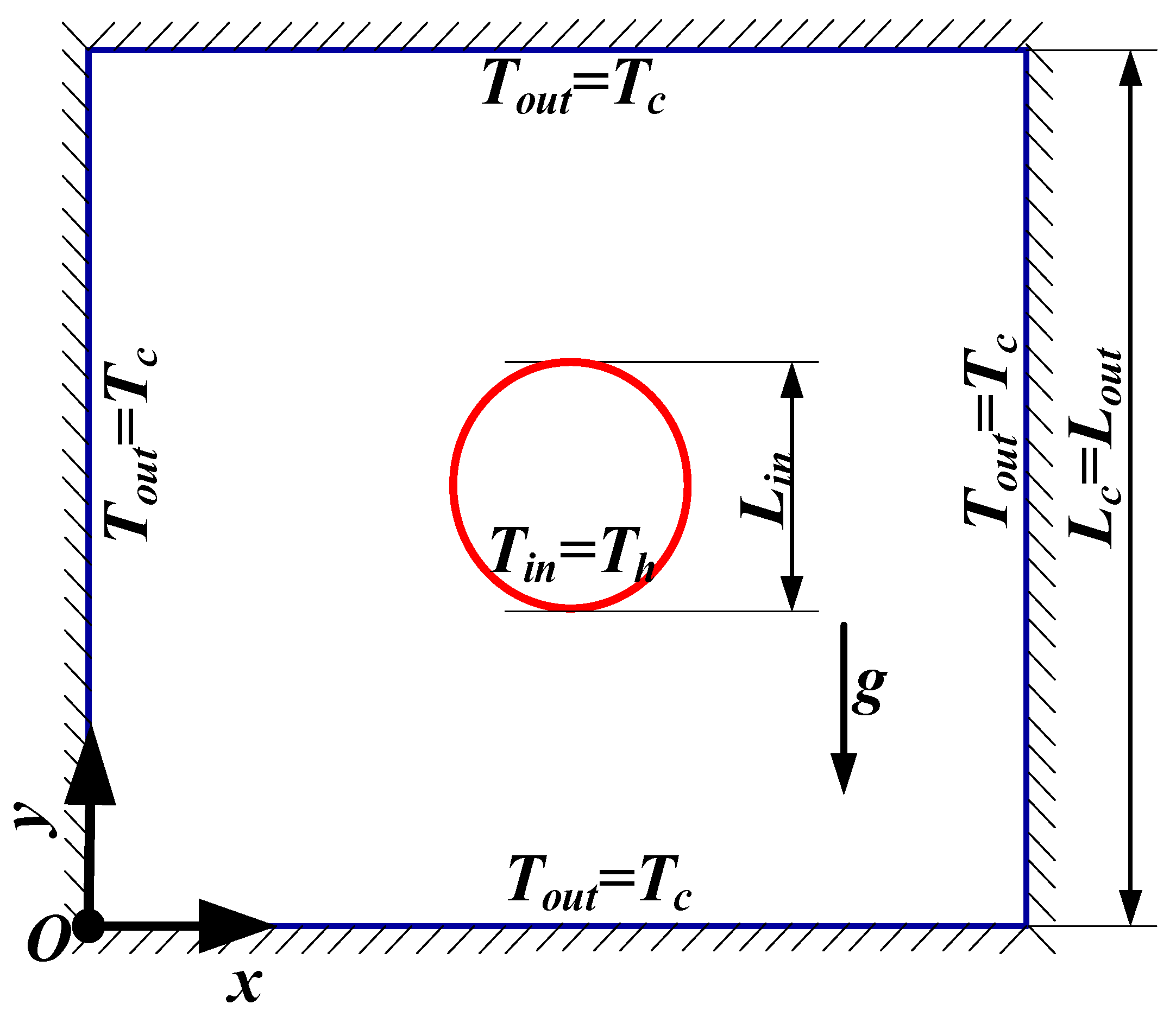
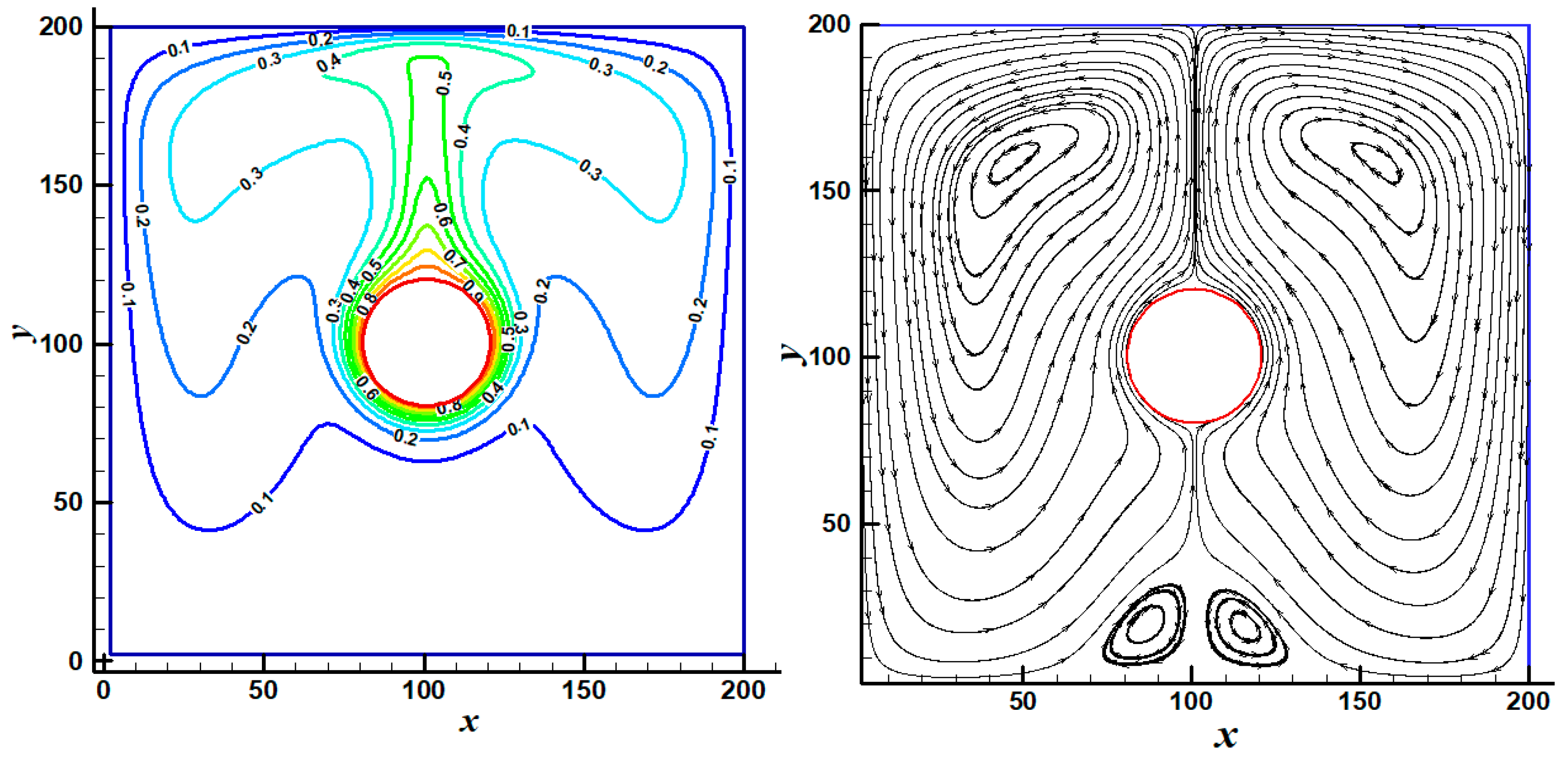
3.1. Validation

The standard benchmarking problem of natural convection due to the hot circular cylinder inside a square enclosure [36,49] is chosen to validate the numerical code developed based on the present simulation technique (see Figure 2 for simulation set-up). The following equation is considered to fix the kinematic viscosity, ν [37]
ν = Pr Ra U c L c ,
where Pr , U c , and L c are the Prandtl number, the characteristic velocity, and the characteristic length, respectively, and the definitions for Ra , Pr , and U c are given by
Ra = g β Δ T L c 3 ν α , Pr = ν α , and U c = g β Δ T L c ,
Δ T in the above equation is the temperature difference between the inner circular cylinder (hot, T i n = T h 1 ) and outer square cavity (cold, T o u t = T h 1 ). The computational domain is divided into 201 × 201 lattice grid points. The simulations are performed for, Pr = 0.71 (i.e., heat transferring medium is air), U c = 0.1 , and L c = L o u t (size of the outer square cavity). Three different combinations for Rayleigh number, Ra = 10 4 ,   10 5 ,   and   10 6 , and the aspect ratio, A R = L i n / L o u t 0.2 ,   0.4 , and 0.6 are considered. Figure 3 shows the isotherms (left side) and streamlines (right side) inside the enclosure when Ra = 10 6 and AR = 0.2. Two symmetrical vortices appear in the upper region of the enclosure, as the natural convection flow intensity is predominant in the upper region of the cavity due to Ra value is very high. The details of the surface-averaged Nusselt number, N ¯ u , on the inner cylinder at all combinations of Ra and AR considered in the present work are provided in Table 1. The corresponding results obtained by the previous works [36,49] are also given in Table 1. N ¯ u increases with Ra for all values of AR. The streamlines and the isotherms patterns, and N ¯ u values of all Ra and AR combinations are in excellent agreement with the previous results [33,35]. After this validation, simulation of fluid flow and heat transfer due to natural convection inside the hexagonal annulus is performed and the corresponding results are discussed in the following section.

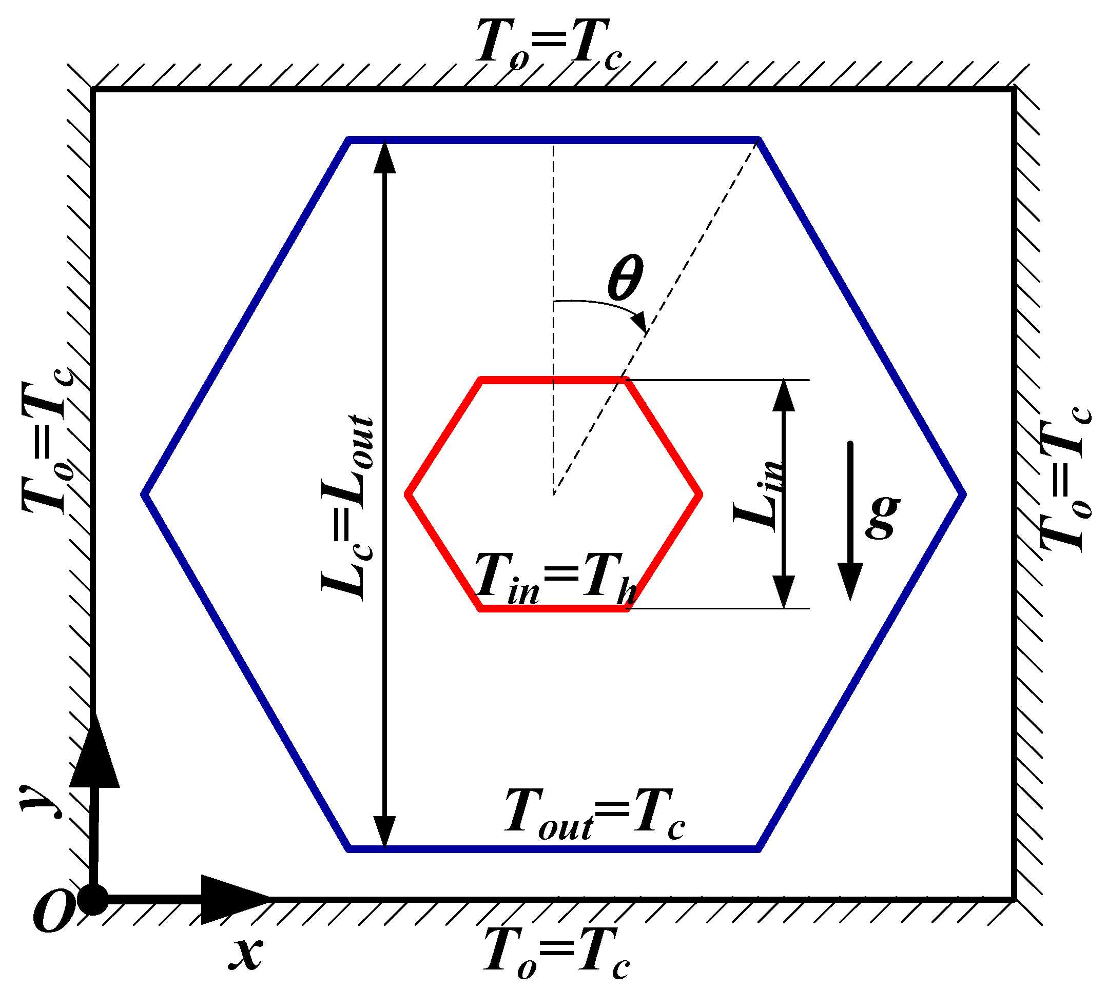
3.2. Natural Convection in the Concentric Hexagonal Annulus

In this session, the results obtained by the simulation of the fluid flow and heat transfer in the annulus bounded by two horizontal concentric hexagonal cylinders are presented (set-up is shown in Figure 1). Simulations are performed for different values of AR and Ra, by varying AR in the range, AR = 0.2~0.6, and Ra in the range, Ra = 10 3 10 6 . The characteristic length in Equation (14) is set as, L c = L o u t (the size of the outer hexagon).
All the results obtained by the present simulation technique are compared with those given by commercial software, ANSYS-Fluent®. Fluent 18.2 is used to simulate a steady laminar flow and heat transfer inside a two-dimensional annular space bounded by two concentric hexagonal cylinders. The size of the outer cylinder is fixed at L o u t = 212   m and that of the inner cylinder is varied as per the AR. The values for the temperatures at the walls of the inner and outer cylinder are set at T i n = 289   K and T o u t = 288   K , respectively. Constant temperature and no-slip BC are used for heat transfer and fluid flow, respectively. The initial value for density is taken as ρ 0 = 1.225   kg / m 3 (air density value at temperature 288 K) and the Boussinesq model is used to model the variation of the density as a function of temperature. Dry air properties at temperature 288 K are used to set the values for specific heat, viscosity, thermal conductivity, and thermal expansion coefficient. The value for the y directional gravitational acceleration constant is varied corresponds to Ra. SIMPLE (Semi-Implicit Method for Pressure Linked Equation) scheme has opted for the pressure-velocity coupling. The governing equations are discretized using the least square cell-based method and a second-order upwind scheme is chosen to solve momentum and energy equations. The Gauss–Seidal iterative method with default under-relaxation factors is selected to solve the system of algebraic equations. The convergence criterion for the residuals of all continuity, momentum, and energy equations is set as 10 9 .

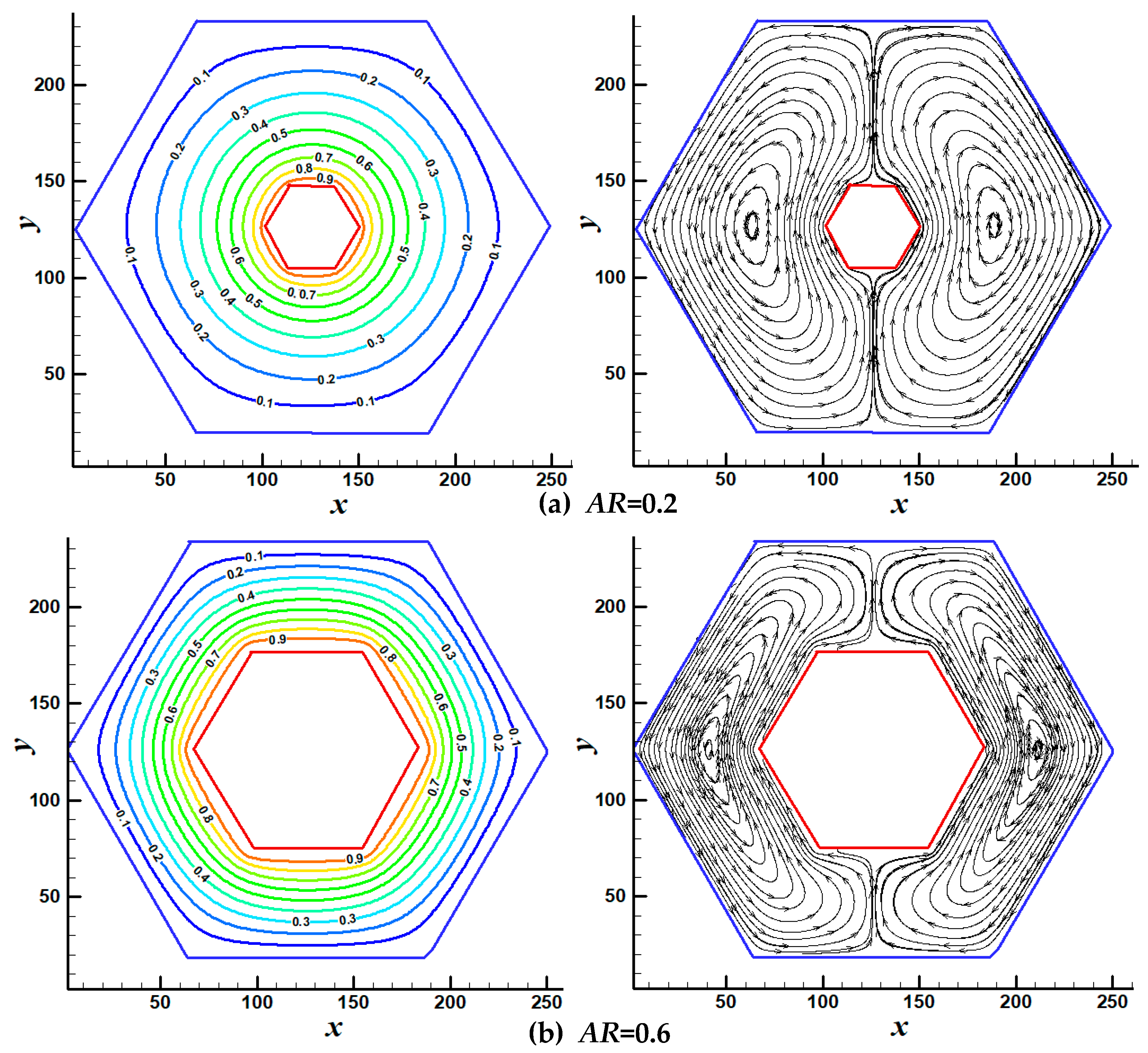
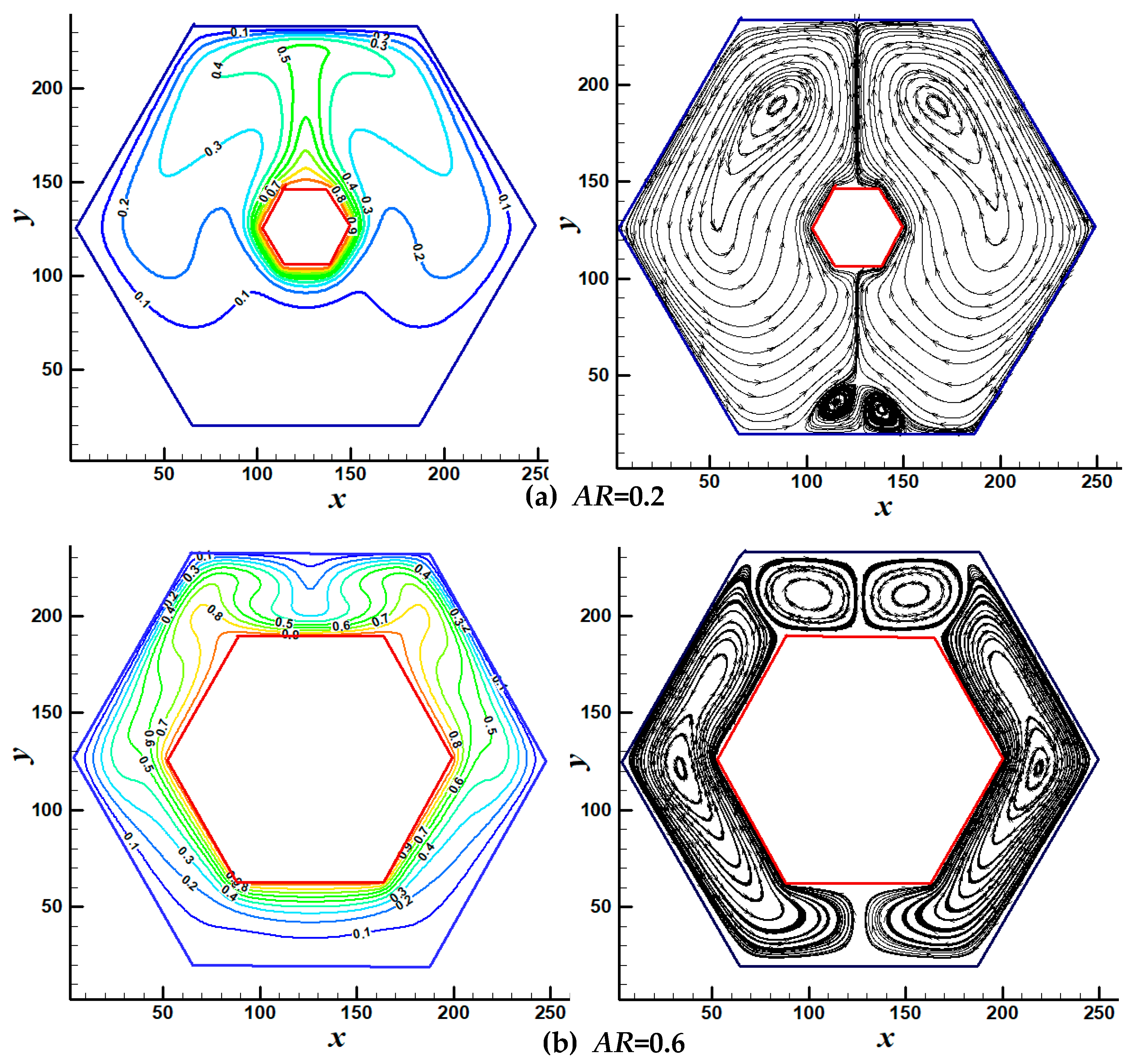
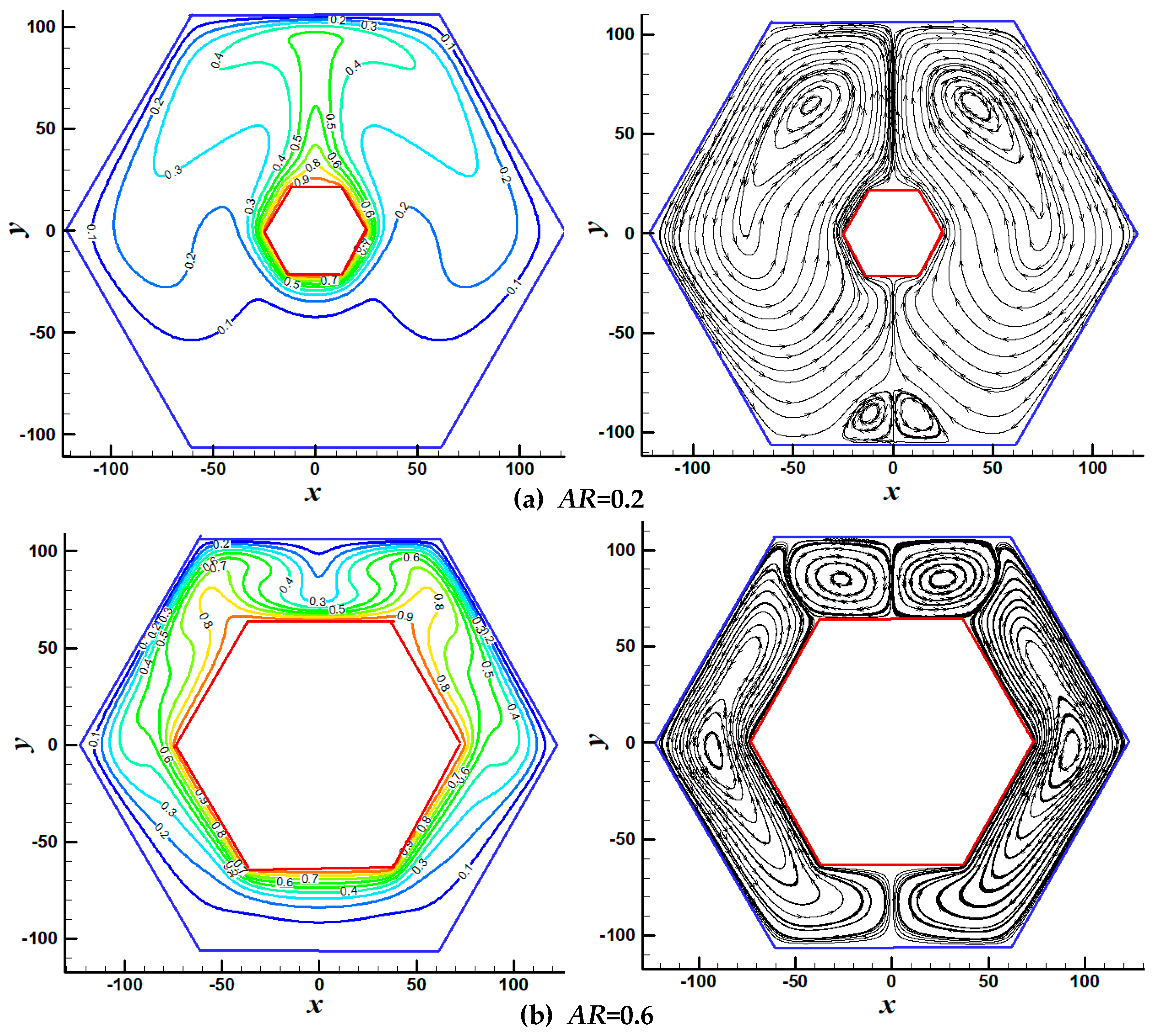
3.2.1. Streamlines and Isotherms Patterns Inside the Annulus

It is observed from the simulation results that irrespective of AR and Ra values, the fluid flow patterns (streamlines) and temperature contours (isotherms) are symmetrical about the vertical centerline of the annulus. Figure 4 shows the isotherms (left side) and streamlines (right side) pattern inside the annulus for the two values of AR = 0.2 (Figure 4a) and AR = 0.6 (Figure 4b), when Ra = 10 3 . As Ra is very low, the strength of the buoyancy force (strength of the gravitational acceleration in this case) that causes the convective flow is very low. Therefore, the heat transfer process inside the annulus is mainly dominated by the conduction mode and the isotherms are very smooth (no distortion of isotherms takes place due to very weak fluid flow) and are almost concentric to the inner and outer hexagonal cylinders. Both isothermal and streamlines are symmetrical concerning the vertical as well as horizontal centerlines of the annulus. When AR = 0.2, the isotherms are almost circular and the spacing between them increases with the distance from the inner hexagon as the available space between inner and outer hexagons is more than that when AR = 0.6. On the other hand, when AR = 0.6, the isotherms in the vicinity of both inner and outer cylinders are in the form of the hexagon and the spacing between them is less as they get squeezed due to constricted space between inner and outer hexagons. The streamlines pattern for both AR = 0.2 and AR = 0.6 show that two symmetrical recirculating eddies (kidney-shaped cells) are formed inside the annulus and the location of cell centers is almost close to the horizontal centerline of the annulus as the fluid flow intensity in the upward direction is almost negligible because of very low Ra. When we observe Figure 4b carefully, we can see that there is slight penetration of the streamline into the solid edges, which is a slight drawback of the present scheme. The main reason for this phenomenon is that as SPM is a non-conforming-mesh method, the same grid system is used for the solid and fluid regions and simulations are also performed inside the solid regions (even though it is enough to consider the boundary effects on the hexagonal edges). However, performing the simulations inside the solid does not affect the flow field in the fluid domain and the overall behavior of the fluid flow and heat transfer is well captured.
Figure 5 shows the isotherms (left side) and streamlines (right side) pattern inside the annulus for the values of AR = 0.2 (Figure 5a) and AR = 0.6 (Figure 5b), and when Ra = 10 6 . As the Ra is very high, the effect of buoyancy-driven flow is significant and hence the heat transfer in the upper region of the annulus is mainly dominated by the convection mode. Isotherms and streamlines are no longer symmetrical about the horizontal median of the annulus. For AR = 0.2, it is concluded from the isotherms and streamlines pattern that the fluid near the inner hexagonal cylinder surface gets heated and moves upwards along the upper inclined edges of the hexagon due to the buoyancy effect. Because of strong convection currents, a thermal plume is formed on the top of the inner cylinder and thermal boundary layer thickness at the top flat edge of the outer cylinder is very thin (indicated by close clustering of isothermal lines) as continuous impingement of fluid flow in the upper region of the annulus. The thermal boundary layer thickness at the bottom of the inner hexagonal cylinder is also found to be very low and the fluid temperature below the inner cylinder is almost uniform and is equal to that of the outer cylinder as heat transfer in this region is dominated by conduction. The centers of the symmetrical recirculating eddies are located well above the horizontal median as the fluid flow is dominant in the upper half of the annulus. The streamline pattern for AR = 0.2 also reveals that two symmetric secondary vortices are formed at the bottom wall of the outer cylinder due to the separation of the momentum boundary layer as a result of strong upward convective flow.
A completely different phenomenon is observed when AR = 0.6. Since there is limited available space for convection on the top of the inner cylinder, two separate thermal plumes (due to the buoyancy-driven fluid flow along the upper inclined edges of the hexagon) are formed along each upper corner of the hexagon. A third thermal plume is also seen on the top flat edge of the inner cylinder in the reverse direction as the uppermost corner of the inner hexagonal cylinder separates the fluid flow and generates two secondary vortices. The fluid flow separation phenomenon can be confirmed by noticing the two counter-rotating cells over the top flat edge of the inner cylinder from the streamline pattern of AR = 0.6. This type of flow separation phenomena at a high AR value was also observed by Raithby et al. [6], Bararnia et al. [30], Moutaouakil et al. [32], and Hu et al. [36], and even though their simulation domains were completely different from the present study.
To assess the capability of the present simulation method for predicting the behavior of natural convection flow in the concentric hexagonal annulus, the results obtained from the present method are compared with ANSYS-Fluent® results. Figure 6 shows the simulation results of isotherms and streamlines patterns obtained from Fluent for the values of AR = 0.2 (Figure 6a) and AR = 0.6 (Figure 6b), and the case when Ra = 10 6 . By comparing the isotherms and streamlines patterns of Figure 5 and Figure 6, we can say that the present simulation results are successfully reproduced the Fluent results.

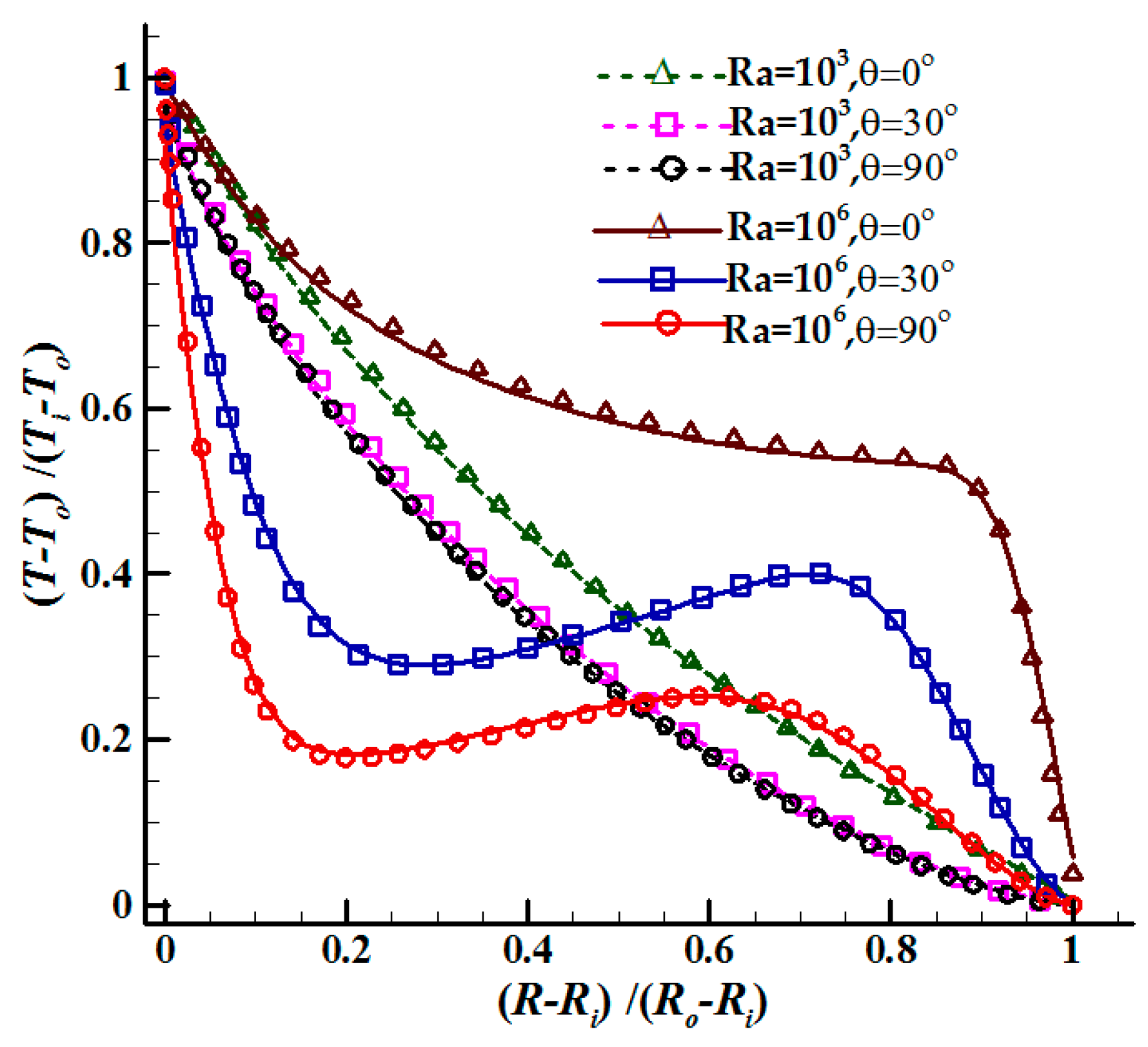
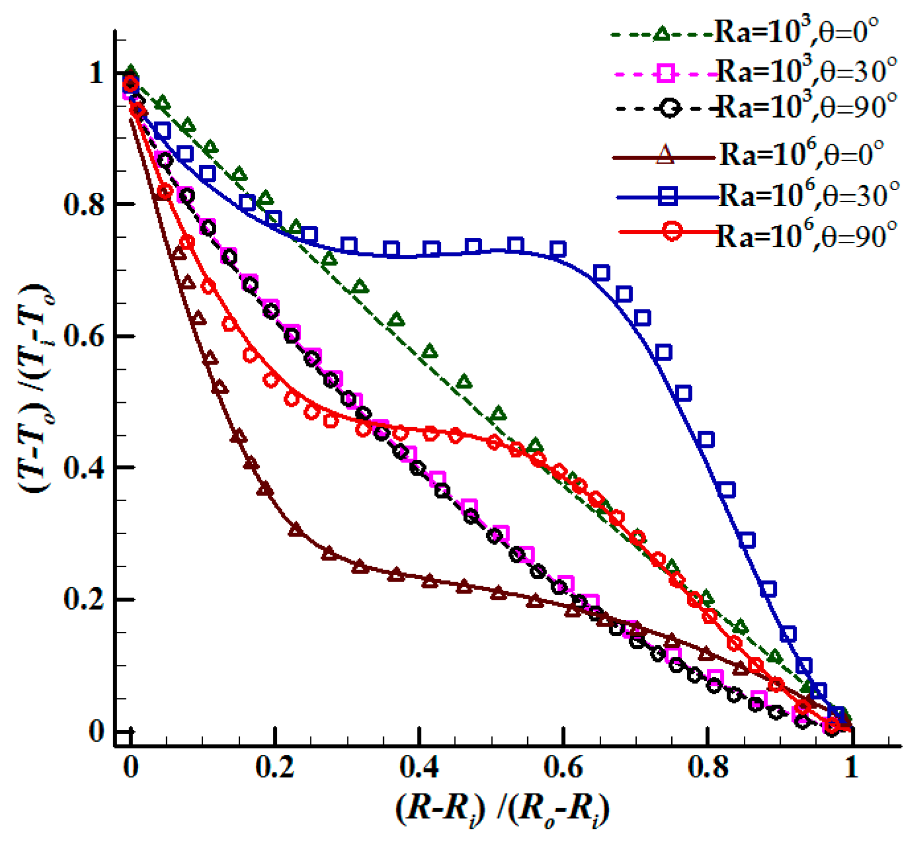
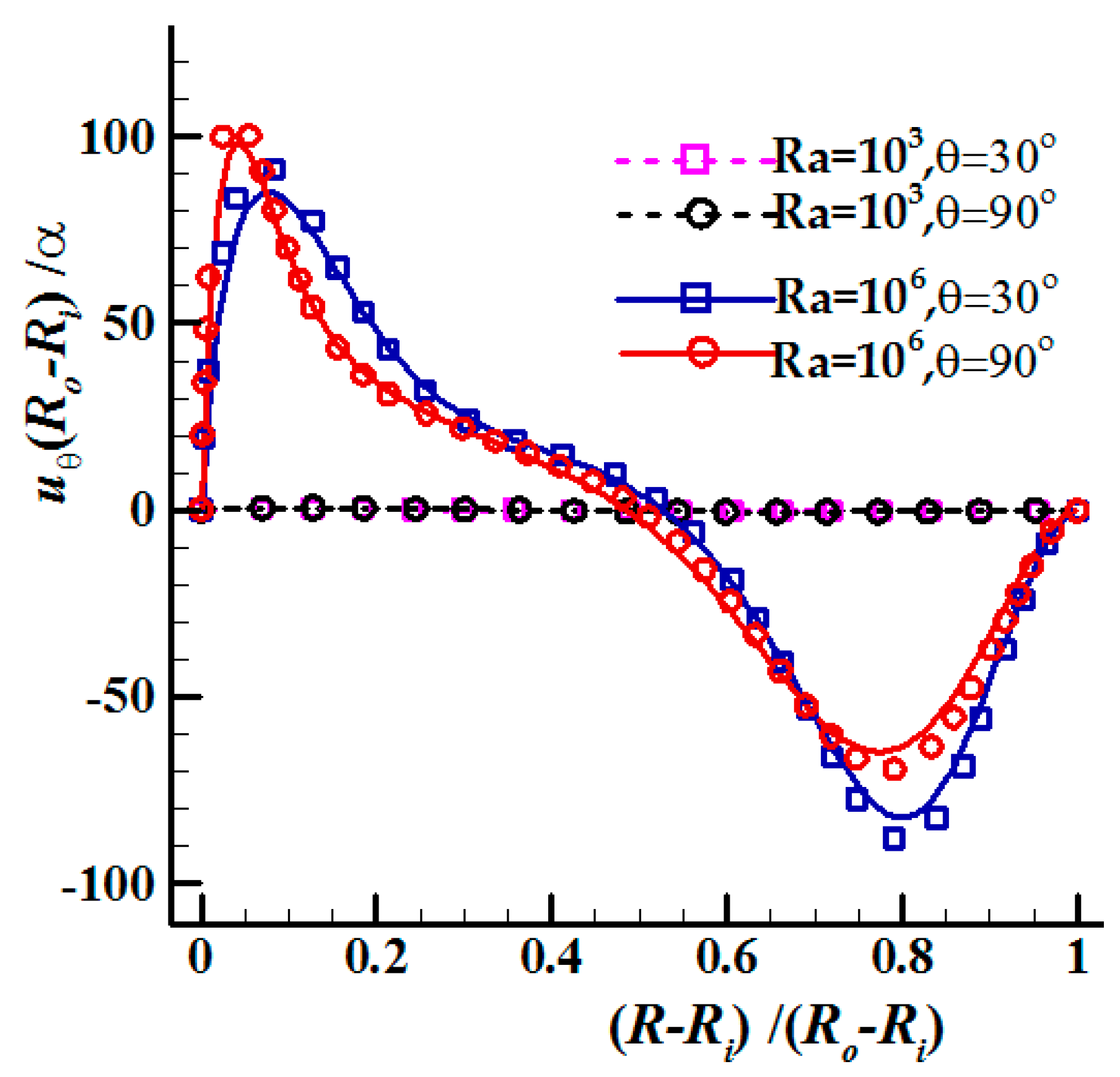
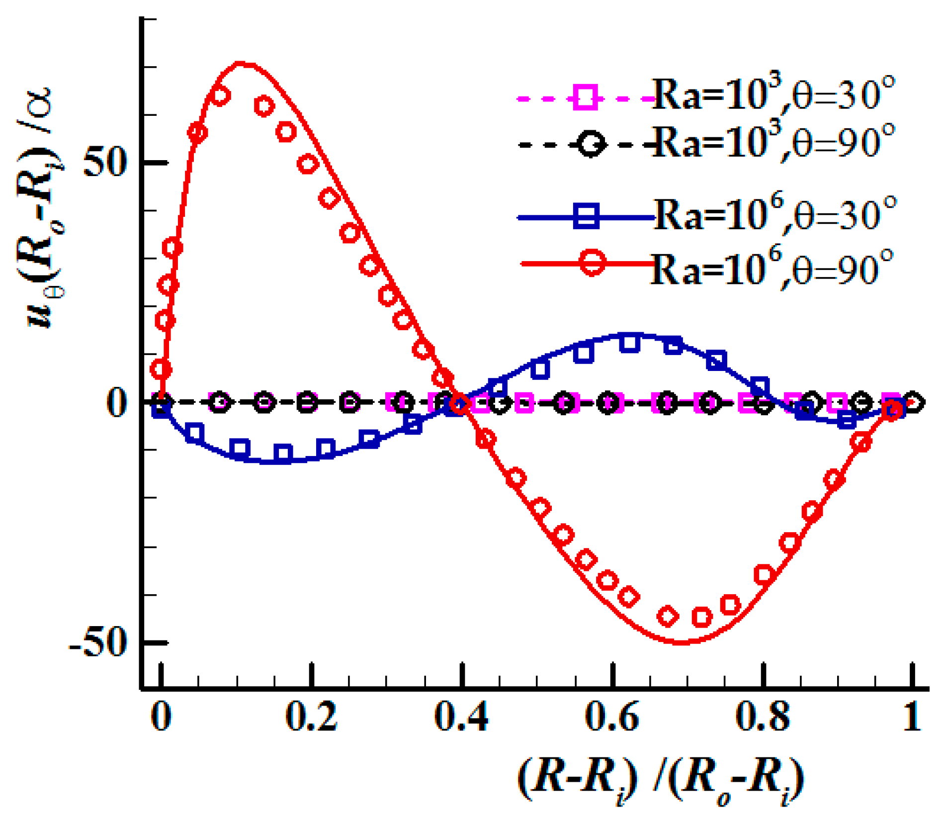
3.2.2. Temperature and Velocity Profiles

Figure 7 shows the temperature distribution along the gap between the inner and outer hexagonal cylinders at three different angular directions, θ = 0 ° (along the line passing through the vertical median), θ = 30 ° (along the line passing through the right uppermost corners of the two hexagons), and at θ = 90 ° (along the line passing through the horizontal median) when AR = 0.2. R i and R o in the figure denote the radius of circles that pass through the edges of inner and outer hexagonal cylinders, respectively. The temperature distribution profiles are plotted for two Rayleigh numbers: Ra = 10 3 and Ra = 10 6 . The symbols in the figure indicate the corresponding results obtained from the Fluent, which are in good agreement with the present simulation results. When Ra = 10 3 , the temperature profiles, along all three θ directions, show a quasi-linear pattern (in other words, the temperature gradients along the gap are almost constant) with the gap as the conduction is the primary mode of the heat transfer process in the annulus. The temperature profiles along θ = 30 ° and θ = 90 ° are almost the same as the isothermal lines are almost concentric and R i values at θ = 30 ° and θ = 90 ° are the same. When Ra = 10 6 , as the strong convective fluid flow disturbs the uniform temperature distribution over the inner hexagon, high-temperature gradients are observed near the inner and outer hexagonal cylinder edges. As mentioned earlier, a thermal plume is formed in the direction of θ = 0 ° for AR = 0.2, the temperature gradients closer to the outer cylinder wall are very steep for the temperature profile along θ = 0 ° as the thermal boundary layer thickness is very thin due to continuous impingement thermal plume against the top flat edge of the outer hexagonal cylinder. The slope of the temperature profile near the outer cylinder wall is steeper for θ = 30 ° compared to that for θ = 90 ° as the convective fluid flow intensity is weaker at θ = 90 ° .
The curves for the temperature distributions along the gap when AR = 0.6 are provided in Figure 8 for Rayleigh numbers, Ra = 10 3 and Ra = 10 6 . The temperature data obtained from Fluent software is also provided (the symbols in the figure) for comparison purposes. The agreement between the two results is excellent, implying the capability of the present simulation technique in the simulation of fluid flow and heat transfer in the hexagonal annuals. In this case, also the slope of the temperature profiles in each θ direction is almost constant when Ra = 10 3 . For Ra = 10 6 case, the temperature profile in the direction of θ = 30 ° is in a similar trend with that of θ = 0 ° of Figure 7 data (for the case of AR = 0.2) as the formation of thermal plume for AR = 0.6 is along the direction of θ = 30 ° . The slope of the temperature profile near the inner cylinder wall is very steep for θ = 0 ° as thermal boundary layer thickness over the flat top edge of the inner cylinder is very small due to the formation of the thermal plume in the reverse direction.
The heat transfer between the outer and inner cylinders is enhanced by convection mode through fluid circulation. The rotational velocity (tangential velocity), u θ , can be used as a good indication for the intensity of the convective fluid flow. Figure 9 shows the variations of tangential velocity, u θ , along the gap between the inner and outer hexagonal cylinders for Rayleigh numbers, Ra = 10 3 and Ra = 10 6 , and for aspect ratio, AR = 0.2. The profiles are plotted for θ = 30 ° and θ = 90 ° . The reference velocity, α / ( R o R i ) , has chosen to normalize u θ . It is noted that the magnitudes of u θ when Ra = 10 3 are very small (almost zero) compared to those when Ra = 10 6 because of a weak fluid flow intensity at low Ra. For the velocity profile at θ = 90 ° , the location of the flow reversal point is exactly at the center of the gap (at the halfway between the corners of two hexagons). However, the flow inversion point for the profile at θ = 30 ° is located a bit away from the gap center towards the outer cylinder. The velocity gradients for the profile at θ = 90 ° are steeper near the inner cylinder than those at the outer cylinder as the convective currents in the region adjacent to the inner cylinder (where fluid gets heated) are stronger than those near the outer cylinder.
The profiles for the tangential velocity distributions when AR = 0.6 are provided in Figure 10 for Rayleigh numbers, Ra = 10 3 and Ra = 10 6 . In this case, as well the magnitudes of u θ when Ra = 10 3 are very small compared to those when Ra = 10 6 . When AR = 0.6, as the thermal plume is formed along the θ = 30 ° direction, the tangential velocity in that direction is very low (fluid flow radially outwards along θ = 30 ° ). Therefore, the magnitude of u θ along θ = 30 ° very low compared to that along θ = 90 ° . The locations for the flow reversal points of the two velocity profiles along θ = 30 ° and θ = 90 ° are the same and are located away from the gap center and are towards the inner cylinder. The magnitudes of u θ obtained for AR = 0.6 case are lower compared to those obtained for AR = 0.2 ( Ra = 10 6 data of Figure 9) as available space for convection flow is constricted at AR = 0.6. The tangential velocity profiles data obtained from the present simulation technique, for cases of AR = 0.2 and AR = 0.6, and Ra = 10 3 and Ra = 10 6 , are compared with those of Fluent software (the symbols in Figure 9 and Figure 10). The present simulation results show good agreement with the Fluent data.

4. Conclusions

In this work, a FORTRAN code based on a hybrid method (which uses a combination of LBM, SPM, and FDM) has been developed to simulate the natural convection inside an annulus between two concentric hexagonal cylinders. After validating the numerical code by applying it to a standard benchmarking problem, natural convection simulations inside the hexagonal annulus have been performed by considering different combinations of Rayleigh number, Ra, and aspect ratio, AR. When AR = 0.6, two separate thermal plumes are formed due to the separation of convective flow at the upper corner of inner hexagon, which is in accordance with the previous studies. To verify the accuracy and robustness of the present method for simulating natural convection flow inside the hexagonal annulus, all the simulation results obtained from the present technique have been compared with the Fluent results. The simulation results of isotherms and streamlines patterns, temperature, and velocity distributions inside the annulus show good agreement with those obtained from Fluent software.

Funding

This research was funded by Kyungsung University Research Grants in 2019 and the APC was funded by the National Research Foundation of Korea (NRF) grant funded by the Korea government (Ministry of Science and ICT) (2020R1G1A1010247).

Acknowledgments

This research was supported by Kyungsung University Research Grants in 2019 and this research was supported by the National Research Foundation of Korea (NRF) grant funded by the Korea government (Ministry of Science and ICT) (2020R1G1A1010247).

Conflicts of Interest

The author declares no conflict of interest.

References

  1. Kuehn, T.H.; Goldstein, R.J. An experimental and theoretical study of natural convection in the annulus between horizontal concentric cylinders. J. Fluid Mech. 1976, 4, 695–719. [Google Scholar] [CrossRef]
  2. Kuehn, T.H.; Goldstein, R.J. An experimental study of natural convection heat transfer in concentric and eccentric horizontal cylindrical annuli. J. Heat Trans. 1978, 100, 635–640. [Google Scholar] [CrossRef]
  3. Boyd, R.D. An Experimental Study on the steady natural convection in a horizontal annulus with irregular boundaries. ASME-HTD 1980, 8, 89–95. [Google Scholar]
  4. Boyd, R.D. A unified theory for correlating steady laminar natural convective heat transfer data for horizontal annuli. Int. J. Heat Mass Transf. 1981, 24, 1545–1548. [Google Scholar] [CrossRef]
  5. Chang, K.S.; Won, Y.H.; Cho, C.H. Patterns of natural convection around a square cylinder placed concentrically in a horizontal circular cylinder. J. Heat Trans. 1983, 105, 273–280. [Google Scholar] [CrossRef]
  6. Raithby, G.D.; Galpin, P.F.; Van Doormaal, J.P. Prediction of heat and fluid flow in complex geometries using general orthogonal coordinates. Numer. Heat Trans. 1986, 9, 125–142. [Google Scholar] [CrossRef]
  7. Glakpe, E.K.; Asfaw, A. Prediction of two-dimensional natural convection in enclosures with inner bodies of arbitrary shapes. Numer. Heat Trans. A 1991, 20, 279–296. [Google Scholar] [CrossRef]
  8. Zhang, H.L.; Wu, Q.J.; Tao, W.Q. Experimental study of natural convection heat transfer between a cylindrical envelope and an internal concentric heated octagonal cylinder with or without slots. ASME J. Heat Trans. 1991, 113, 116–121. [Google Scholar] [CrossRef]
  9. Peskin, C.S. Flow patterns around heart valves: A numerical method. J. Comp. Phys. 1972, 10, 252–271. [Google Scholar] [CrossRef]
  10. Glowinski, R.; Pan, T.-W.; Helsa, T.; Joseph, D.D. A distributed lagrange multiplier/fictitious domain method for particulate flows. Int. J. Multiph. Flow. 1999, 25, 755–794. [Google Scholar] [CrossRef]
  11. Nakayama, Y.; Yamamoto, R. Simulation method to resolve hydrodynamic interactions in colloidal dispersions. Phys. Rev. E. 2005, 71, 036707-1–036707-7. [Google Scholar] [CrossRef] [PubMed] [Green Version]
  12. Luo, X.; Maxey, R.M.; Karniadakis, G.E. Smoothed profile method for particulate flows: Error analysis and simulations. J. Comp. Phys. 2009, 228, 1750–1769. [Google Scholar] [CrossRef]
  13. Alapati, S.; Che, W.S.; Suh, Y.K. Simulation of sedimentation of a sphere in a viscous fluid using the lattice Boltzmann method combined with the smoothed profile method. Adv. Mech. Eng. 2015, 7, 794198-1–794198-12. [Google Scholar] [CrossRef] [Green Version]
  14. Succi, S. The Lattice Boltzmann Equation for Fluid Dynamics and Beyond; Oxford University Press: Oxford, UK, 2001. [Google Scholar]
  15. Alapati, S.; Kang, S.M.; Suh, Y.K. Parallel computation of two-phase flow in a microchannel using the lattice Boltzmann method. J. Mech. Sci. Technol. 2009, 23, 2492–2501. [Google Scholar] [CrossRef]
  16. Di Palma, P.R.; Huber, C.; Viotti, P. A new lattice Boltzmann model for interface reactions between immiscible fluids. Adv. Water Resour. 2015, 82, 139–149. [Google Scholar] [CrossRef]
  17. Chen, G.; Huang, X.; Wang, S.; Kang, Y. Study on the bubble growth and departure with a lattice Boltzmann method. China Ocean Eng. 2020, 34, 69–79. [Google Scholar] [CrossRef]
  18. Dellar, P. Lattice Kinetic Schemes for Magnetohydrodynamics. J. Comp. Phys. 2002, 179, 95–126. [Google Scholar] [CrossRef]
  19. Dellar, P. Lattice Boltzmann formulation for Braginskii magnetohydrodynamics. Comput. Fluids 2011, 46, 201–205. [Google Scholar] [CrossRef]
  20. Fyta, M.; Melchionna, S.; Succi, S.; Kaxiras, E. Hydrodynamic correlations in the translocation of biopolymer through a nanopore: Theory and multiscale simulations. Phys. Rev. E 2008, 78, 036704-1–036704-7. [Google Scholar] [CrossRef]
  21. Alapati, S.; Fernandes, D.V.; Suh, Y.K. Numerical simulation of the electrophoretic transport of a biopolymer through a synthetic nanopore. Mol. Simulat. 2011, 37, 466–477. [Google Scholar] [CrossRef]
  22. Alapati, S.; Fernandes, D.V.; Suh, Y.K. Numerical and theoretical study on the mechanism of biopolymer translocation process through a nanopore. J. Chem. Phys. 2011, 135, 055103-1–055103-11. [Google Scholar] [CrossRef] [PubMed]
  23. Hu, Y.; Li, D.C.; Shu, S.; Niu, X.D. Modified momentum exchange method for fluid-particle interactions in the lattice Boltzmann method. Phys. Rev. E 2015, 91, 033301-1–033301-14. [Google Scholar] [CrossRef] [PubMed]
  24. Yuan, H.Z.; Niu, X.D.; Shu, S.; Li, M.J.; Yamaguchi, H. A momentum exchange-based immersed boundary-lattice Boltzmann method for simulating a flexible filament in an incompressible flow. Comput. Math. Appl. 2014, 67, 1039–1056. [Google Scholar] [CrossRef]
  25. Kohestani, A.; Rahnama, M.; Jafari, S.; Javaran, E.J. Non-circular particle treatment in smoothed profile method: A case study of elliptical particles sedimentation using lattice Boltzmann method. J. Dispers. Sci. Technol. 2020, 41, 315–329. [Google Scholar] [CrossRef]
  26. Zhang, Y.; Pan, G.; Zhang, Y.; Haeri, S. A relaxed multi-direct-forcing immersed boundary-cascaded lattice Boltzmann method accelerated on GPU. Comput. Phys. Commun. 2020, 248, 106980. [Google Scholar] [CrossRef]
  27. Sheikholeslami, M.; Bandpy, M.G.; Ganji, D.D. Magnetic field effects on natural convection around a horizontal circular cylinder inside a square enclosure filled with nanofluid. Int. Commun. Heat Mass. 2012, 39, 978–986. [Google Scholar] [CrossRef]
  28. Sheikholeslami, M.; Bandpy, M.G.; Ganji, D.D. Lattice Boltzmann method for MHD natural convection heat transfer using nanofluid. Powder Technol. 2014, 254, 82–93. [Google Scholar] [CrossRef]
  29. Lin, K.-H.; Liao, C.-C.; Lien, S.-Y.; Lin, C.-A. Thermal lattice Boltzmann simulations of natural convection with complex geometry. Comput. Fluids 2012, 69, 35–44. [Google Scholar] [CrossRef]
  30. Bararnia, H.; Soleimani, S.; Ganji, D.D. Lattice Boltzmann simulation of natural convection around a horizontal elliptic cylinder inside a square enclosure. Int. Commun. Heat Mass. 2011, 38, 1436–1442. [Google Scholar] [CrossRef]
  31. Sheikholeslami, M.; Bandpy, M.G.; Vajravelu, K. Lattice Boltzmann simulation of magnetohydrodynamic natural convection heat transfer of Al2O3-water nanofluid in a horizontal cylindrical enclosure with an inner triangular cylinder. Int. J. Heat Mass Transf. 2015, 80, 16–25. [Google Scholar] [CrossRef]
  32. Moutaouakil, L.E.; Zrikem, Z.; Abdelbaki, A. Lattice Boltzmann simulation of natural convection in an annulus between a hexagonal cylinder and a square enclosure. Math. Probl. Eng. 2017, 2017, 3834170-1–3834170-11. [Google Scholar] [CrossRef] [Green Version]
  33. Hu, Y.; Niu, X.-D.; Shu, S.; Yuan, H.; Li, M. Natural convection in a concentric annulus: A lattice Boltzmann method study with boundary condition-enforced immersed boundary method. Adv. Appl. Math. Mech. 2013, 5, 321–336. [Google Scholar] [CrossRef]
  34. Hu, Y.; Li, D.; Shu, S.; Niu, X. Immersed boundary-lattice Boltzmann simulation of natural convection in a square enclosure with a cylinder covered by porous layer. Int. J. Heat Mass Transf. 2016, 92, 1166–1170. [Google Scholar] [CrossRef]
  35. Khazaeli, R.; Mortazavi, S.; Ashrafizaadeh, M. Application of an immersed boundary treatment in simulation of natural convection problems with complex geometry via the lattice Boltzmann method. J. Appl. Fluid Mech. 2015, 8, 309–321. [Google Scholar] [CrossRef]
  36. Hu, Y.; Li, D.; Shu, S.; Niu, X. An efficient smoothed profile-lattice Boltzmann method for the simulation of forced and natural convection flows in complex geometries. Int. Commun. Heat Mass. 2015, 68, 188–199. [Google Scholar] [CrossRef]
  37. Alapati, S.; Che, W.S.; Ahn, J.-W. Lattice Boltzmann method combined with the smoothed profile method for the simulation of particulate flows with heat transfer. Heat Transfer Eng. 2019, 40, 166–183. [Google Scholar] [CrossRef]
  38. Ladd, A.J.C. Numerical simulations of particulate suspensions via a discretized Boltzmann equation. Part 1. Theoretical foundation. J. Fluid Mech. 1994, 271, 285–309. [Google Scholar] [CrossRef] [Green Version]
  39. Ladd, A.J.C. Numerical simulations of particulate suspensions via a discretized Boltzmann equation. Part 2. Numerical results. J. Fluid Mech. 1994, 271, 311–339. [Google Scholar] [CrossRef] [Green Version]
  40. Bouzidi, M.; Firdaouss, M.; Lallemand, P. Momentum transfer of a Boltzmann-lattice fluid with boundaries. Phys. Fluids 2001, 13, 3452–3459. [Google Scholar] [CrossRef]
  41. Yu, D.; Mei, R.; Luo, L.-S.; Shyy, W. Viscous flow computations with the method of lattice Boltzmann equation. Prog. Aerosp. Sci. 2003, 39, 329–367. [Google Scholar]
  42. Mittal, R.; Iaccarino, G. Immersed boundary methods. Ann. Rev. Fluid Mech. 2005, 37, 239–261. [Google Scholar] [CrossRef] [Green Version]
  43. Marshall, K.N.; Wedel, R.K.; Dammann, R.E. Development of Plastic Honeycomb Flat-Plate Solar Collectors; Lockheed Missiles & Space Company Inc.: Palo Alto, CA, USA, 1976. [Google Scholar]
  44. Buchberg, H.; Edwards, D.K.; Mackenzie, J.D. Transparent Glass Honeycombs for Energy Loss Control; School of Engineering and Applied Science, University of California: Los Angeles, CA, USA, 1977. [Google Scholar]
  45. Marin, O.; Vinuesa, R.; Obabko, A.V.; Schlatter, P. Characterization of the secondary flow in hexagonal ducts. Phys. Fluids 2016, 28, 125101. [Google Scholar] [CrossRef]
  46. Aliabadia, M.K.; Deldarb, S.; Hassanic, S.M. Effects of pin-fins geometry and nanofluid on the performance of a pin-fin miniature heat sink (PFMHS). Int. J. Mech. Sci. 2018, 148, 442–458. [Google Scholar] [CrossRef]
  47. Sadasivam, R.; Manglik, R.M.; Jog, M.A. Fully developed forced convection through trapezoidal and hexagonal ducts. Int. J. Heat Mass Transf. 1999, 42, 4321–4331. [Google Scholar] [CrossRef]
  48. Zhang, L.Z. Transient and conjugate heat and mass transfer in hexagonal ducts with adsorbent walls. Int. J. Heat Mass Transf. 2015, 84, 271–281. [Google Scholar] [CrossRef]
  49. Moukalled, F.; Acharya, S. Natural convection in the annulus between concentric horizontal circular and square cylinders. J. Thermophys. Heat Trans. 1996, 10, 524–531. [Google Scholar] [CrossRef]
Figure 1. Simulation set-up for investigating the natural convection in an annulus region between two concentric hexagonal cylinders. The origin of the lattice grid is mentioned by ‘O’ in the figure.
Mathematics 08 01043 g001
Figure 2. Set-up, consists of an annular space between an outer square enclosure (cold) and an inner circular cylinder (hot), considered for validating the present numerical method.
Mathematics 08 01043 g002
Figure 3. Isotherms (left side) and streamlines (right side) patterns inside the square enclosure when Rayleigh number is, Ra = 10 6 , and aspect ratio, AR = 0.2.
Mathematics 08 01043 g003
Figure 4. Isotherms (left side) and streamlines (right side) patterns inside the hexagonal annulus when the Rayleigh number is, Ra = 10 3 , and for AR = 0.2 (a), and AR = 0.6 (b).
Mathematics 08 01043 g004
Figure 5. Isotherms (left side) and streamlines (right side) patterns inside the hexagonal annulus when the Rayleigh number is, Ra = 10 6 , and for AR = 0.2 (a), and AR = 0.6 (b).
Mathematics 08 01043 g005
Figure 6. Isotherms (left side) and streamlines (right side) patterns obtained from ANSYS-Fluent® software for the values of AR = 0.2 (a) and AR = 0.6 (b) when Ra = 10 6 .
Mathematics 08 01043 g006
Figure 7. Temperature distribution along the gap between the inner and outer hexagonal cylinders at different angular directions, θ = 0 ° , θ = 30 ° , and at θ = 90 ° for AR = 0.2. The symbols represent corresponding data from Fluent software.
Mathematics 08 01043 g007
Figure 8. Temperature distribution along the gap between the inner and outer hexagonal cylinders at angular directions, θ = 0 ° , θ = 30 ° , and at θ = 90 ° for AR = 0.6. The symbols represent corresponding data from Fluent software.
Mathematics 08 01043 g008
Figure 9. Variation of tangential velocity, u θ , along the gap between the inner and outer hexagonal cylinders at angular directions, θ = 30 ° , and θ = 90 ° for AR = 0.2. The symbols represent the corresponding data from Fluent software.
Mathematics 08 01043 g009
Figure 10. Variation of tangential velocity, u θ , along the gap between the inner and outer hexagonal cylinders at angles, θ = 30 ° , and θ = 90 ° for AR = 0.6. The symbols represent the corresponding data from Fluent software.
Mathematics 08 01043 g010
Table 1. The details of the surface average Nusselt number, N ¯ u , on the inner cylinder at different combinations of Ra and AR.
RaARPresentPrevious [36]Previous [49]
1040.22.0422.0352.071
0.43.2023.1733.331
0.65.3495.2665.826
1050.23.7143.7513.825
0.44.8434.8935.080
0.66.1826.1756.212
1060.25.9596.1156.107
0.48.7188.8979.374
0.611.66211.94011.620

