A Dynamic Study of Biochemical Self-Replication


Department of Chemistry, Williams College, Williamstown, MA 01267, USA
*
Author to whom correspondence should be addressed.
†
The authors contributed equally to this work.
Mathematics 2020, 8(6), 1042; https://doi.org/10.3390/math8061042
Submission received: 3 May 2020
/
Revised: 20 June 2020
/
Accepted: 24 June 2020
/
Published: 26 June 2020
(This article belongs to the Special Issue Advanced Mathematics for Physical Chemistry and Chemical Physics)
Abstract
:As it is well understood, in biological systems, small regulatory motifs are present at all scales, thus looking at simple negative feedback loops give us some information of how autocatalytic systems may be affected by regulation. For a single template self-replication, we consider a plausible mechanism, which we reduce to a 2-variable dimensionless set of ordinary differential equations, (ODE). The stability analysis of the steady states allows us to obtain exact relations to describe two-parameter bifurcation diagrams. We include a negative feedback to the reactants input to study the effect of regulation in biochemical self-replication. Surprisingly, the simpler regulation has the largest impact on the parameter space.
MSC:
34C25; 37G15; 92B05; 92E991. Introduction
During the early 1900s, Bray [1] reported periodic changes, which we now refer as damped oscillations, in the catalytic decomposition of hydrogen peroxide. Interesting enough, Lotka’s 1910 paper [2] reported such damped oscillations, but Lotka’s or Bray’s work did not motivate the study of chemical oscillations. It took until the 1950s, when Belousov [3] first, and Zhabotinskii [4] later, reported a chemical system that showed periodic changes over a period of an hour, the now so-called BZ reaction. Namely, both Belousov and Zhabotinsky considered a simple solution of an organic acids and bromate in the presence of an inorganic catalyst. Belousov considered critic acid and cerium(V) sulfate, while Zhabotinsky considered malonic acid and two catalysts, cerium(IV) and iron(II). The citric acid reaction develops into a turbid solution, while the malonic acid develops into a clear solution. Although the systems considered were closed, periodic color changes were observed, yellow ⇌ colorless for citric acids, while for malonic acid, showed the combination of four colors: yellow ⇌ colorless and red ⇌ blue. As we know, due to the second law of thermodynamics, the concentrations of reactants and products cannot vary periodically, but the periodic color changes are due to the catalyst, which show two oxidation states, and each with a particular color.
During the 1960s the interest on chemical oscillations grew considerably [5,6,7,8,9,10], and now, we find that periodic changes are found in many physical, biological, chemical, physiological and ecological systems, and the study of nonlinear dynamics has developed into a major field of research. In particular, studies of oscillating biochemical systems have recently gained profound popularity [11,12,13,14,15,16,17,18,19]. In the case of biochemical reactions, it was recognized that at least one reaction or a subset of reactions need to show autocatalysis. In other words, the product of a reaction should increase its own production, and in mathematical terms, the Jacobian associated with the dynamic system should have positive diagonal terms to show oscillations.
For biochemical oscillating systems, autocatalysis plays a central role, but in general it has been a topic of great interest. In particular, researchers have considered a small number of reagents that can yield a compound that can self-replicate. The simplest system has two reactants and one product, which serves as a template of its own synthesis. This idea has been explored for nucleotides [20,21,22,23,24,25], organic compounds in non-aqueous solvents [26,27,28,29,30,31,32], modified ribozymes [33,34,35] and peptides [36,37,38,39,40,41,42,43,44,45]. As we mentioned earlier, growth of the self-replicating compound is necessary for any system to evolve, and it has been observed in a handful of compounds. In particular we have focused our work on the ribozyme system developed by Joyce et al. [33,34,35], where the system shows an exponential growth.
In this study, we introduce an extension of a minimal model, the so-called Templator model [46,47,48,49,50,51], as a means by which we can study the behavior of biochemical self-replication. Our objective is to propose a robust mathematical model that adequately predicts the outcome of the reaction and takes into account the variation of certain parameters. To obtain the mathematical model, we make a number of assumptions. For example, temperature changes in the system are negligible and the reactions solutions are well stirred. We also assume that the rate constants in the reaction mechanism of the individual elementary reactions may follow certain relations that make the analysis of the system more tractable. Taking all these assumptions into consideration, we were able to analyze a set of ordinary differential equations associated with the proposed mechanism.
For a ribozyme system, we consider, in Section 2, a bimolecular mechanism of the formation of the product, which serves as template for an autocatalyzed reaction. In contrast with our previous work [46,47,48,49,50,51], where we studied a minimal model, we, in Section 3, consider the full model and derive exact relations among the parameters to determine the conditions required by the Poincare–Andronovo–Hopf (PAH) bifurcations. In Section 4, we discuss the time behavior of the solutions and their correlation with the two-parameter bifurcation diagrams. In Section 5, we look at a self-regulated chemical self-replication, considering in particular its bifurcation diagrams in Section 6. Finally, we discuss our results in Section 7, and summarize our findings in Section 8.
2. Mechanistic Approach
In previous work [46,47,48,49,50,51], we have considered Reberk’s [26,27,28,29,30,31,32] and Joyce’s [33,35] self-replicating system and modeled self-replication using a self-complementary template mechanism. For this mechanism, we use a reasonable chemical model that is consistent with laboratory results on self-replication [33,35]. In particular, we consider a simple self-replicating mechanism; however, in general, the following mechanistic steps can represent self-replication:
where P represents the self-replicating molecule and A and B are the component fragments. This set of mechanistic steps, obviously, imply simplifications to an underlined mechanism of elementary reactions, but is commonly used to analyze the rate of production of P and to check if the rate of formation of P is linear in the concentration of the product.
In the initiation step, components A and B interact with a relative low probability to form the template, P. The structure of the product P is such that once it is formed, it preferentially binds A and B in a conformation that facilitates covalent bonding between the A and B molecules to form another P molecule. The newly created product and the original molecules then split apart and independently catalyze further reactions. The rate of the reaction has been experimentally studied [33] for low reactant concentrations an expressed as a pseudo first order process,
where is a pseudo first order rate constant that depend on the initial concentrations of the reactants.
Once the exponential growth is experimental stablished, one can now consider a detailed set of elementary reactions. For example, we study the following underlying mechanism:
in which case all of the above elementary reactions are reversible, the forward and backward reactions of each step having rate constants. The final step in the mechanism is taken to be the rate determining step, meaning that the rate should be first order with the respect to the intermediate I.
In the experimental systems of Reberk’s [26,27,28,29,30,31,32] and Joyce’s [33,35], the reactant concentrations are in the range of micromolar (M) to 100 M. Therefore, we can use the standard mean field approach and use the Mass Action Law to express the discrete events in terms of ordinary differential equations involving the reactants concentrations. In other words, since the experimental concentrations are large enough, we do not have to include any low number stochastic description. Consequently, assuming that the rates of each of the reactions consuming the intermediates I, and are variables such that the rate of change of the concentrations of these species, at any moment, are essentially zero, we can use a system of three algebraic equations, in the so-called steady state approximation. From the above reaction mechanism and the respective rate constants, we get the following differential equations:
The three equations can be solved simultaneously to give the symbolic value for I in terms of the constants and the concentrations A, B, P. None of the intermediate concentrations are measurable in the time scale of the experiments that are able to measure the concentrations of A, B and T. Therefore, expressing it in terms of measurable and known quantities is an important step in determining a theoretical rate equation that matches the experimental one. Solving for I, we get
As far as we know, values of the individual rate constants, in particular for the elementary steps involving fast variable, have not been reported for the specific experimental systems included in our study. Moreover, if rate constants are reported, the values are associated with the rates of the slow variables. At least for ribozymes and peptide systems, there is no experimental evidence of cooperativity that may imply that the rate constants may be all different. Since the values of the individual rate constants are difficult to measure or have not been reported, we can make some reasonable assumptions that can make the subsequent analysis simpler. For example, in the simplest case, two scenarios can occur here; no path preference, which means that the steps undertaken when undergoing the upper route are similar to the corresponding steps in the bottom route, hence . No cooperation or allosteric effects implies that the individual steps are independent of each other, and therefore the rate constants of subsequent steps, in each route, are the same, which means the the rate constants satisfy the following relations: .
In the latter case, the assumption is that the mechanism undergoes a symmetric and noncooperative scheme. Taking this assumption into account, we can now simplify the expression for the concentration I to:
where and . In previous work, we have used Equation (6) to analyze Joyce’s batch system and found that the approximations give a reasonable dynamic description of the publish data. Furthermore, we have used the same approximations in our studies of artificial peptide networks [52,53,54,55] in batch and open conditions with similar success.
To analyze the mechanism in detail, we need to determine how the concentration of the reactants and products vary as function of time. To do this, we have to model the reaction mechanism in terms of differential equations. As mentioned before, the overall reaction itself occurs as described by Equation (1). So far, we have obtained the relevant relations for the self-replicating mechanism, we want to consider an open system, where the self-replicating dynamics are central to our analyses. At this point, where one wants to model the dynamics, in most cases chemist use the so-called chemical pool approximation [15,16,17,18,19], where one considers a constant reservoir with and concentrations, usually in the micromolar range (M). From this reservoir, the reactants are continuously pumped into the reaction mixture at a constant rate , usually in the range of 10–100 mL per hour. Another interpretation of the chemical pool approximation assumes the presence in excess of a precursors, and , that decays with a rate . We emphasize that this the most common first approximation used by chemist to analyze the dynamics of reaction mechanism, in our case a self-replicating mechanism. Once one considers the chemical pool approximation and gains some insight on the effect of the mechanism in the dynamics, one can consider other experimental conditions like the continuous stirred tank reactor, (CSTR), or a regulated inflow.
In the case of chemical pool approximation, to model the reactant’s input, we can describe the process as follow:
After including an input, we need to consider an output to study the self-replicating mechanism as an open system. As in our previous work, we assume that the product P is removed from the reaction mixture through a certain two-step enzymatic process,
Considering all the steps, we simplify our original differential equations into the following three
where
The above differential equations define the concentrations of the reactants and products as the reaction progresses. However, these three equations can be reduced if we consider the following simple relations:
In this case we only consider the average and difference of the concentrations of A and B.
The ODEs for these new variables reduce to the following relations:
If we consider only experiments where there is no dominant reagent, it means that the concentrations and are equal, which means that at any time Y is a constant. Keeping this condition in mind, we obtain only two ODEs
These equation can further simplify into:
where and .
The above equations contain several parameters that have to be taken into account during analysis. To reduce the number of parameters without diminishing the quality of the analysis we scale the above equations to get a pair in which the parameters are dimensionless. Using the following scaling:
we obtain the differential equations shown below.
where we define the following dimensionless parameters:
with defined . These constitute the Templator model of self-replicating molecules.
After considering simple bimolecular processes followed by simple self-replicating chemical systems and include some kinetic simplifications, we obtain a two variable dimensionless set of ODEs that characterize the dynamics of chemical self-replication. The model has been compared with the batch reacting system of ribozymes [34], to estimate the parameter values that we use in our previous work.
3. Stability Analysis
To analyze the dynamical behavior of the system described by Equations (16a) and (16b), we first have to find the steady sates of the system. To do this, we equate the rate of change of concentration of each reactant to zero and solve the subsequent simultaneous equations. So we first find the steady states and find the following relations: relations:
where we notice that .
Taking these relations into account, we find that the coefficient of is always positive. Likewise, the coefficient of is also always positive. However, the coefficient of x is always negative and so is the constant term. This proves that the signs of the coefficients in the expression, no matter what the values of the parameters are, only change once from positive to negative. We can see that the above cubic equation has one real positive root because the signs of the coefficients of x in the expression change only once. After solving numerically, the cubic equation we get three solutions, from which we can pick the one real positive solution, .
The stability of the the steady state is determined by the trace of the Jacobian. So we find first the relaxation/Jacobian matrix J of our ODEs to be:
Next we calculate the trace of the Jacobian at the steady state. The zeros of the trace are given by the zeros of the following polynomial
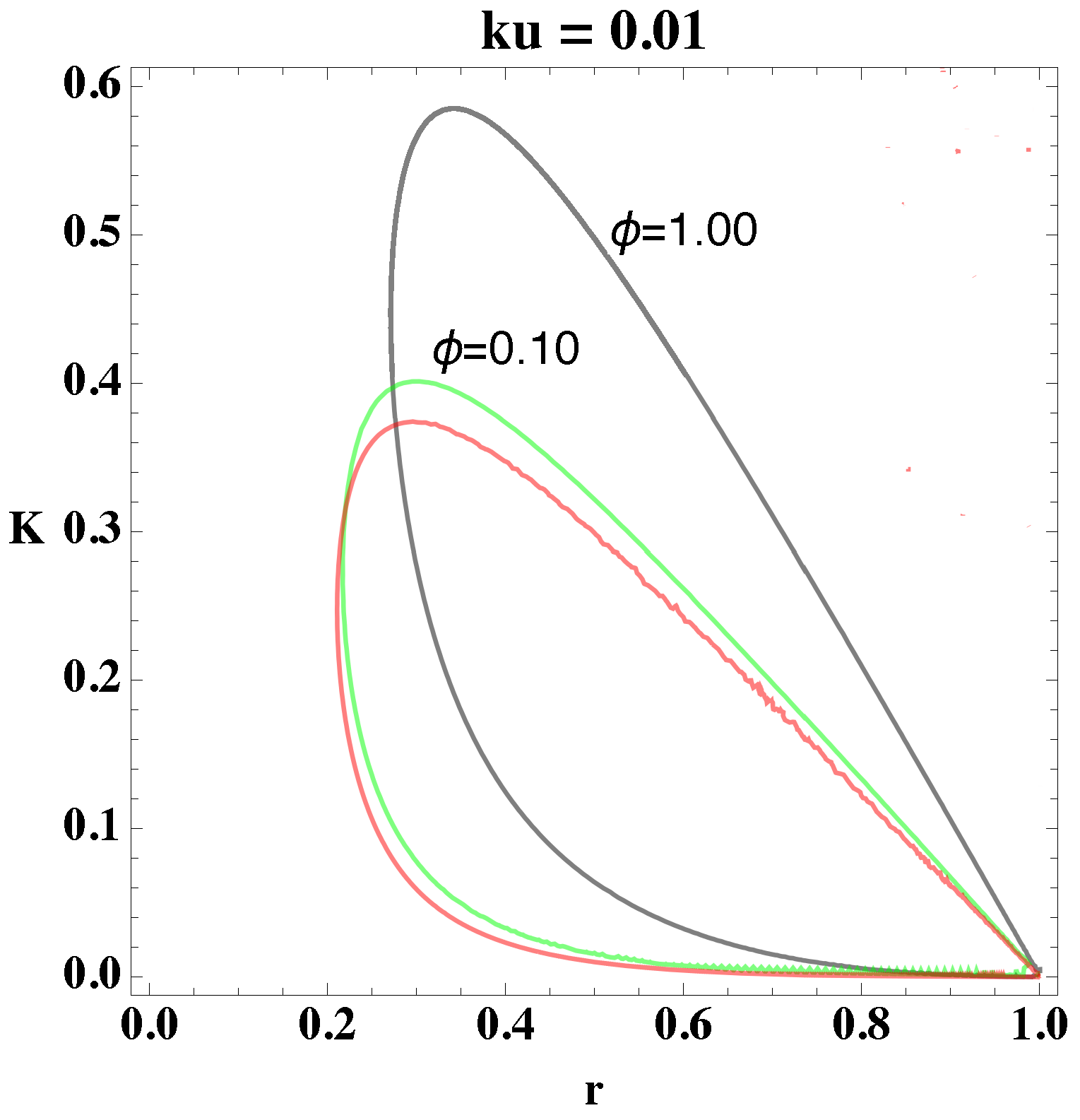
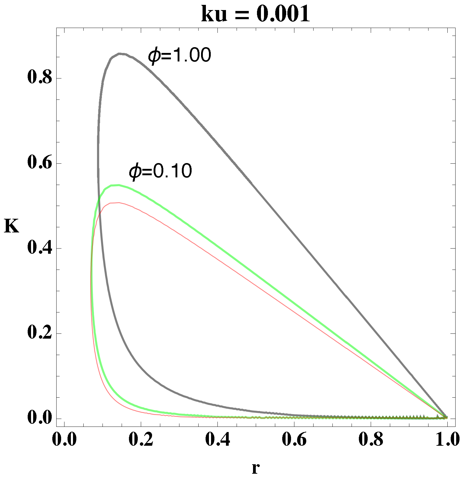
First, from Equation (18b) we determine the solution as a function of r and K and substitute its value in Equation (20), to obtain a function that includes only the parameters r and K. Consequently, we can determine the two-parameter bifurcation diagram that indicates how the parameters relate to each other. Using these procedures, we determine the bifurcation diagram, which we depict in Figure 1 and Figure 2. In the former figure, we depict the two-dimensional plots of K versus r for different values, and in the latter figure, we consider .
From Figure 1 and Figure 2, we select a combination of parameter values, (, that yield stable oscillations. In both figures, the bounded region represents the values in which the systems become unstable, that is, the values of the parameters that give oscillations. Every point that lies outside the bounded area represents either damped oscillations or a steady state. Picking parameter values that lie within the bounded region, therefore, will lead to a reaction in which the concentrations of the reactants and products oscillate in time.
Moreover, from Figure 2, we notice that as the value of increases, the area in parameter space, i.e., bounded region, shifts upwards and increases the interval of parameter values. The figures show the overall change in the bifurcation diagram only for small values of . However, for small values of (i.e., 0.01) the behavior of the loop is generally as depicted in Figure 1 and Figure 2. Experiments show that the value of the rate constant , of the uncatalyzed reaction, is usually an order of magnitude smaller than of the catalyzed reaction, which implies, physically, that .
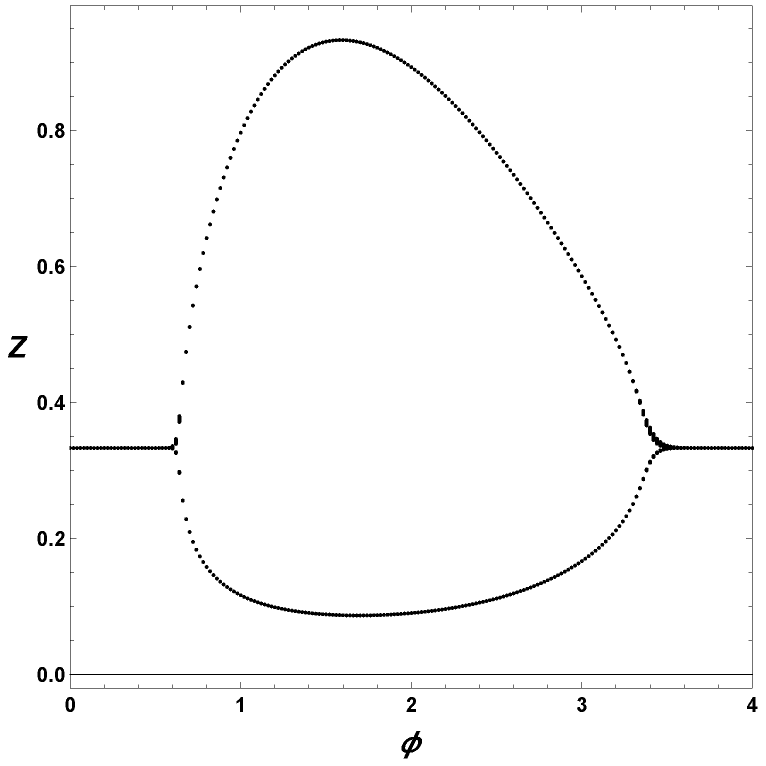
Finally, to understand the effect of , we construct a extrema Poincare section in Figure 3. For this diagram, we first consider a set of parameter values, , and , and integrated the ODEs for different values of the bifurcation parameter, in this case . From the integrated solutions, we collected the minima and maxima. Therefore, in Figure 3, we plot the extrema of Z as a function of . The upper branch represents the maxima, and the lower branch the minima, thus we are considering the amplitude of the oscillations. Notice from Figure 3 that the maximum amplitude occurs about , and, also, that the minima are relatively away from the zero values.
4. Time Series
In interpreting the following diagrams it is helpful to consider the actual quantitative relationship to the physical world that the diagrams have. To do so, we need to connect the dimensionless numbers that are shown on the diagrams with the actual experimental data. When scaling down the differential equations, we defined the following relationship between X and x:
The physical units for the concentration X are M while the corresponding quantity x is dimensionless. Therefore, by definition, we require that:
This expression can be simplified to
and, using to the data collected from the experiment by Paul and Joyce [34], we find the following relationship:
Since the values of A and B used were 2 M for each reactant, the value for is approximately equal to
Using the following relationship for time,
and plugging in the values for and calculated above, we get the following relationship between the time (t) in min and the dimensionless time () in Equation (15c), min.
Therefore, in the following figures, values measured on the -axis should be multiplied by 25 min to convert them into physical time units.
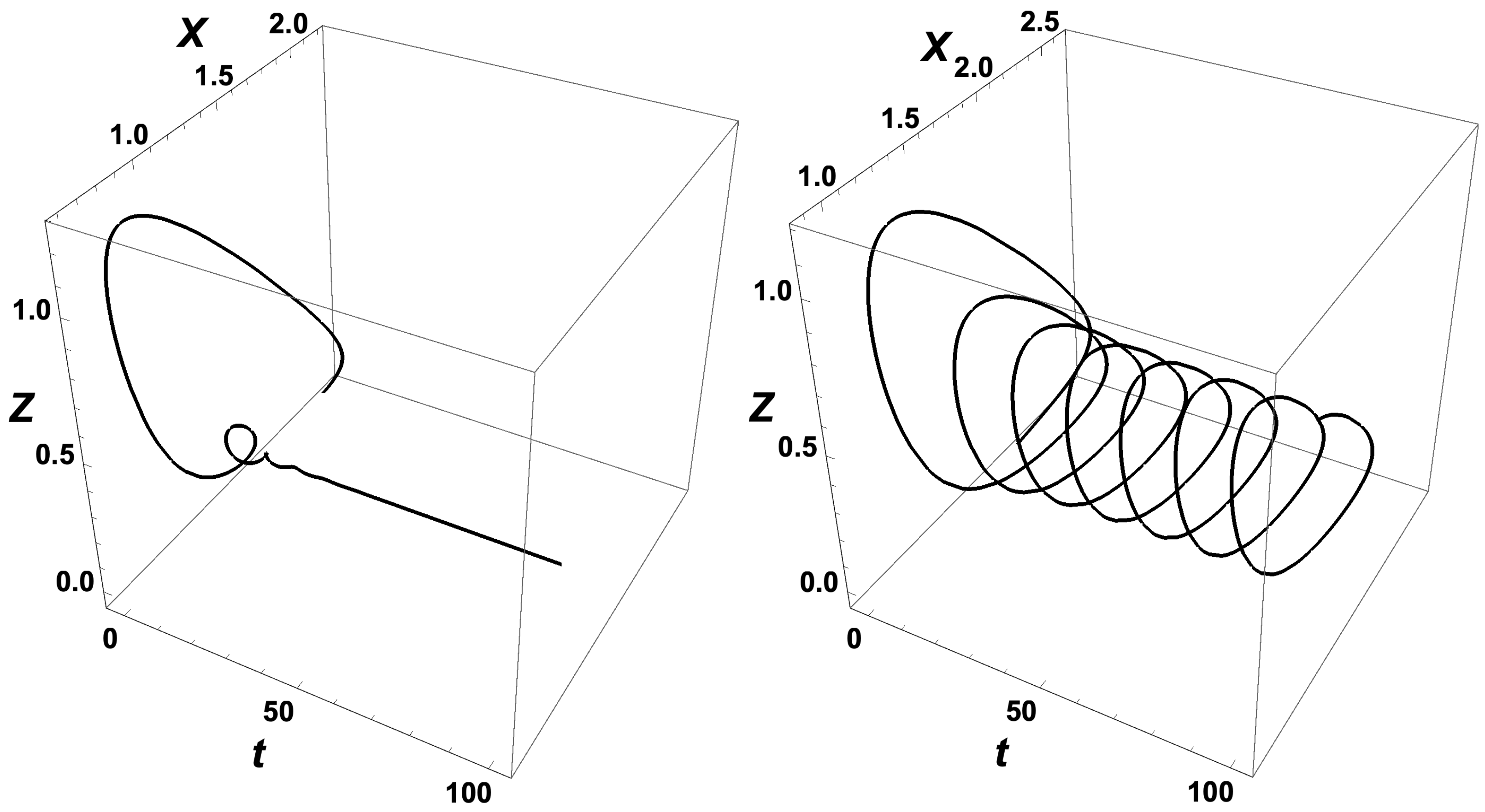
The importance of the inclusion of in the analysis is demonstrated by the change in the area of the loop when the value of is varied. Figure 1 shows that the loops and have a significant area of intersection, and an equally significant unshared portion. By picking parameter values within this region, we can show that merely altering the value of can change the behavior of the system, i.e., generate oscillations or eliminate them. For example, if we pick the point (0.50, 0.40) from Figure 1 and change we can see a transition from no oscillations to clear, to oscillations. Figure 4 depicts the effect of .
In our previous work [46,47,48,49,50,51], we assumed that the parameter was too small to be of any considerable effect. However, in this analysis, we decided to include it to determine how much its presence would affect the expected dynamics. As discovered above, the parameter is important since its inclusion can help clarify why oscillations are observed where they were previously not expected, and why they are not where they previously were. The extent to which this parameter affects the bifurcation diagrams highlights this importance. However, the analysis also shows that the inclusion of does not affect the results at a qualitative level. For example, the bifurcation diagrams generated in this case are closed loops, whether is considered or not. Oscillations are also observed even if is not included. This means that the original model, where the parameter is ignored, is still useful if the mechanism is simply being consulted to explain some qualitative phenomena, for example, the presence of chemical oscillations. It is only when greater detail is required, that the revised equations have to be used. When a quantitative analysis needs to be executed, the revised model is recommended, lest subtle anomalies be encountered.
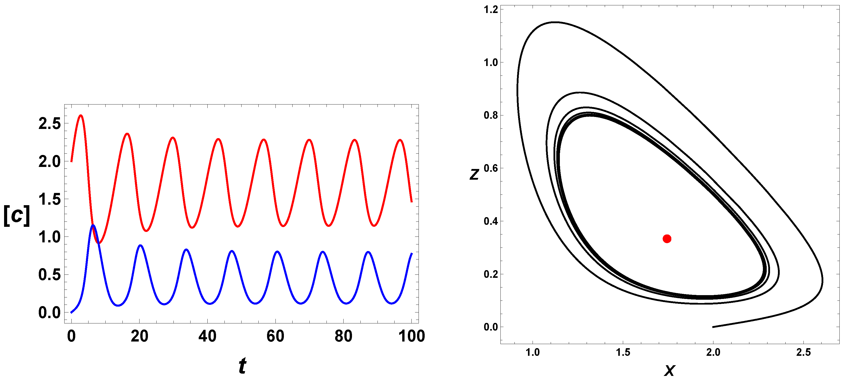
Furthermore, from Figure 5, the period of the oscillations calculated (3–5 h) is of the order of magnitude of the experiments reported by Lincoln and Joyce [35], although the latter experiment was not under constant pumping. This fact also adds credit to the validity of the model. In addition, the Templator model proposed above goes through two bifurcations when either K or r is varied as in Figure 1 and Figure 2. This property coincides with the experimental observation that biochemical systems are able to sustain oscillations for parameter values within a bounded interval of parameter values.
5. Self-Regulation
In System Biology studies, researchers have found in genetic and metabolic networks the presence of feedback motifs. In particular, autocatalysis [52,53,54,55] can be considered as a positive feedback. In our case, our positive feedback (chemical self-replication) linked with a constant input of reactants and an enzymatic sink yields stable oscillations. From System Biology, we also find a common regulatory combination of motif links a positive feedback with negative feedback, which in many cases is a self-repressive feedback. Moreover, these two feedbacks yield oscillations. In our case, self-replication under open conditions yields oscillations, but we want to explore the effects of auto-repression.
In the case of genetic networks, researchers have used Hill functions to model activation or repression, and in many case one has to add a leak term [56]. In this section, we want to study the effect of a negative feedback on the reactants input. So far, we considered a constant input, which is the so-called chemical pool approximation. The simplest possible functional form is a Hill function, with exponent equal to unity. We notice that in the case of genetic networks, researchers usually use n values greater than unity, . To simplify the analysis, we consider the minimal Templator model, .
In previous section, we use a constant input, described by parameter r, and now we want to modify the input as follows, , where
Therefore we get the following set of ODEs:
where is the simplest functional form of the negative feedback.
To find the steady states, in general and as long as the input function only depend on z, we can solve for z as a function of the parameters, since the steady states satisfies the following relation:
For our choice of regulated input, we find the following polynomial:
Once we solve for , we can solve of x, using the following relation:
Consequently, we can get expressions for the steady states as functions of the the parameters.
The stability of the steady states is related to the trace of the Jacobian,
which, four set of ODEs, reduces to a polynomial of z.
Notice that the relation described by Equation (33) is explicitly independent of the input function, , but it depends implicitly through the z dependence of Equation (29). Thus, in general, for any input function, , we can solve for z as a function of the parameters, and use Equation (33) to determine a two-parameter bifurcation diagram.
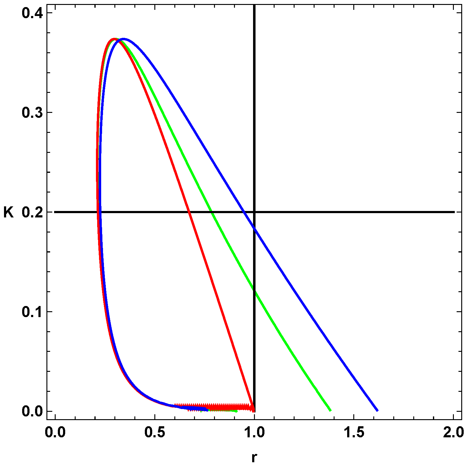
In Figure 6, we considered the simplest case, where , and (blue) and (green). The figure depicts the effect of the negative feedback on the parameter space. The red curve represents no regulation and constant input, or the so-called minimal Templator model. The blue line is associated with the simplest possible negative regulation, the green contour represents the case with . We recall that for the minimal model, the r values are limited to the interval (0,1), with unphysical concentrations for . Therefore, we first notice that the simple negative regulation, , increases the parameter space for stable oscillations, and second, in that respect, does a better job that the case . Although, the K values associated to stable oscillations are about the same, the r values are strongly affected by the negative regulation of the input function. Thus, a regulated self-replicating system has a larger parameter space for allowed stable oscillations, including values of r greater that unity, and depicted by the vertical line . The horizontal line shows the effect on the values of r for , but the effect on r is more noticeable for small values of K.
6. Poincare Sections
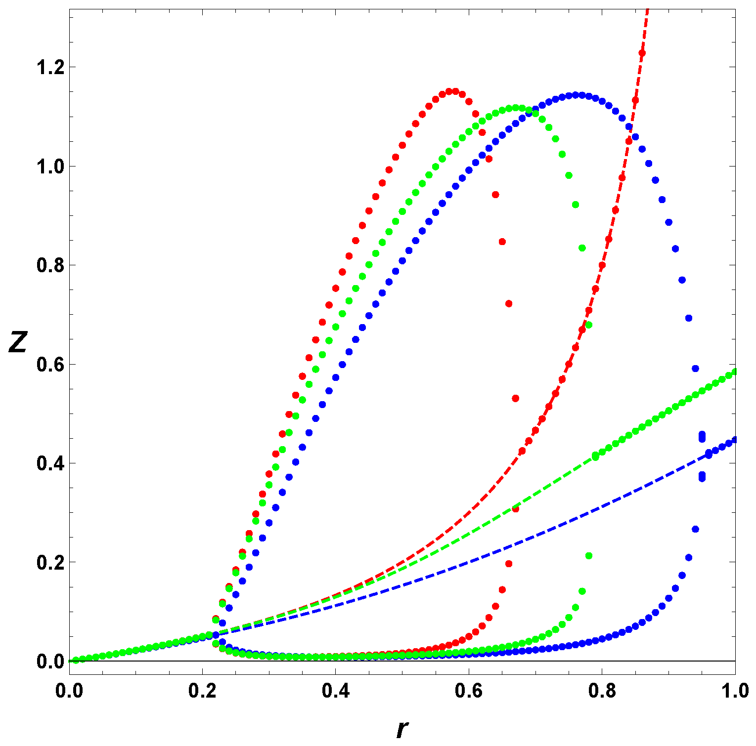
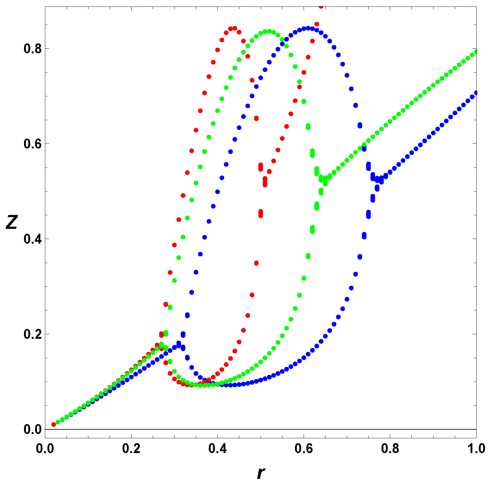
In this section, we consider some Poincare section of extrema. As we mention earlier, in this case, we integrate the ODEs, and look for the maxima and minima of the numerical solutions. In contrast from previous section, we include several values of . To appreciate separately the effect of the regulation and the usage of the full model, , we first consider in Figure 7 the minimal Templator model, , for , and . For these parameters, we can refer to horizontal line in Figure 6, which shows the increase of values, r, but it does not tell us the effect on the oscillation amplitudes.
Figure 7 depicts the maxima and minima of the stable oscillations for different values of the bifurcation parameter, in this case r. As seen from Figure 6 the minimal model, in red, has a smaller range of values of r and the steady state diverges as r approaches unity. The regulated cases do not show any divergence in the steady state values. Furthermore, the cases and show that the simple regulation, does a better job increasing the interval of values of r yielding stable oscillations the case , the regulation do not affect noticeably the amplitude of the stable oscillations, but regulation smooths the PAH bifurcations, in particular the second PAH bifurcations.
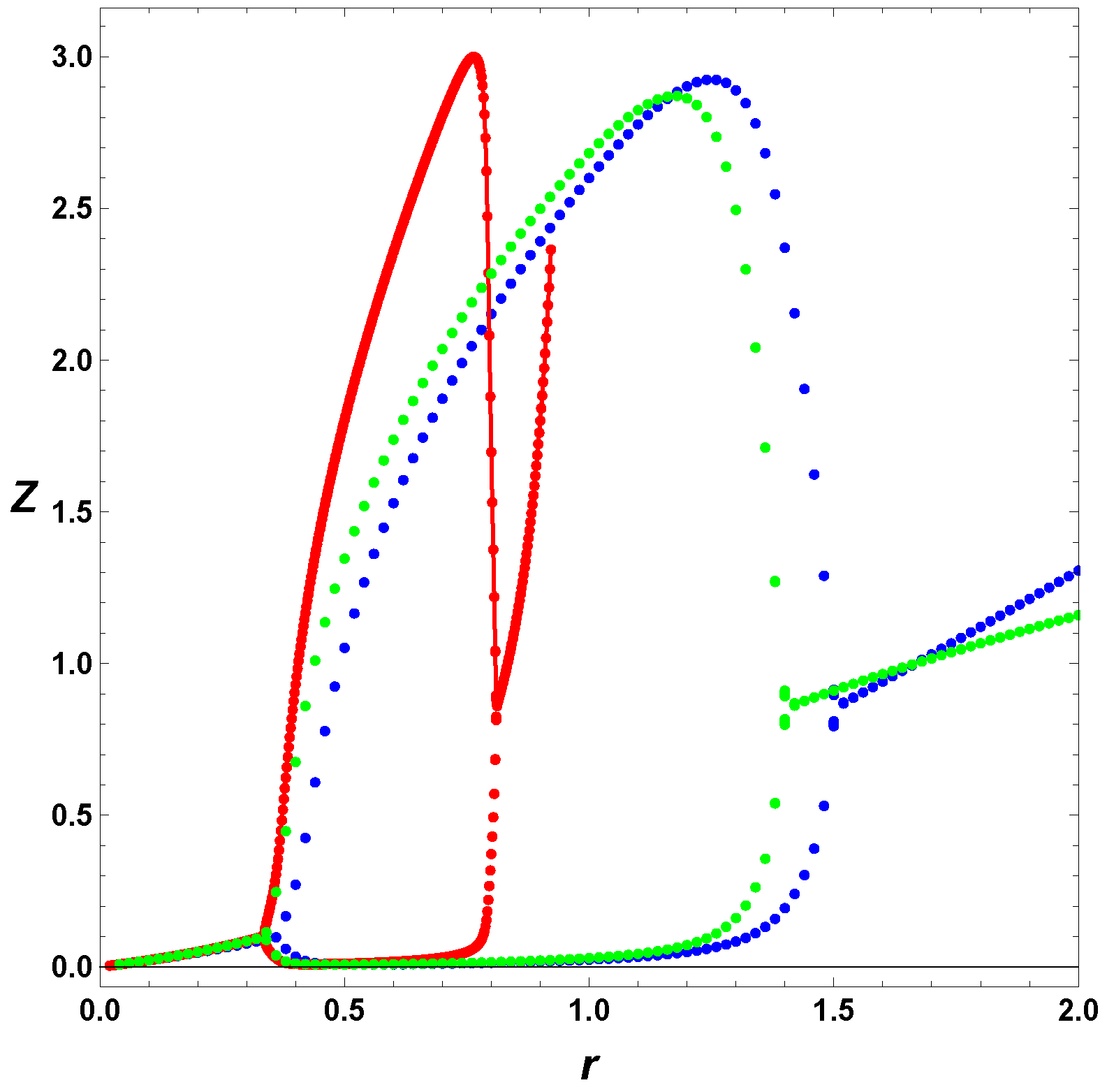
Next, we, in Figure 8, consider the effect of regulation in the full Templator model, . As in the case of the minimal model, negative regulation increases the parameter space, in particular the interval for r values, including values greater than unity that are forbidden for the minimal model. As before, regulation smooths the second PAH bifurcation in contrast to the sharp change in amplitude displayed by the minimal model in red.model in red.
Finally in Figure 9, we include the full Templator model, and change the value of , which, for the minimal model, shows only a steady state behavior. For this case, we notice the same effect as in the other cases. The full model, , expand the parameter space, but regulation, which can also have the same effect on the parameter space, it also smooths the second PAH bifurcation, probably avoiding a Canard bifurcation. Although, the minimal model and the full model have similar dynamic behaviors, the minimal is used as a qualitative approach to self-replication, while the full model should be use in the case of an experimental set up.
7. Discussion
Over the years, researchers have emphasized the relevance of autocatalysis and its relation to potential models of the origin of life [52,53,54,55,56,57,58,59,60,61,62,63,64]. Therefore, we extend our previous work with a minimal Templator model [46,47,48,49,50,51] to analyze in detail a more general mechanistic model of self-replication, as in the case of modified ribozymes [33,34,35] that use a simple template mechanism, usually known as first order or singlet self-replication, which distinguishes from the second order or duplex self-replication shown by peptides [36,37,38,39]. For our extended model, we use the steady state approximation to eliminate the fast variable, and to obtain a set of dimensional ODEs. We further scale the ODEs to obtain a set of dimensionless equations, knowing that the autocatalyzed reaction is much faster than the uncatalyzed. Finally, we consider, as in experimental conditions, stoichiometric input and initial conditions, so we end with a two-variable dimensionless system of ODEs, which is the Templator model for first order chemical self-replication.
For the Templator model under open conditions, we determine the two-parameter, , diagram for the PAH bifurcation, and consider the differences between the minimal and the full model, to find that the qualitative properties are similar, differing only on the quantitative level. The main difference is the effect on the parameters space, , which is larger for the full model compare with the minimal model. In other words, the Templator shows stable oscillations, where the minimal model does not. Consequently, we may want to use the minimal model, because the algebraic manipulations are easier to obtain a qualitative general dynamic description of a generic system related to a specific experimental system of reacting reagents. If one has a direct access to experimental data of a particular chemical system, the full model is more adequate to correlate the dynamic behavior of the model with the experimental system.
As we mentioned earlier, biochemical self-replications, or in general positive feedbacks such as autocatalysis, are prevalent in biochemical networks, which can be described by the interaction of smaller feedback loops. Among the relevant motifs found in the large genetic or metabolic networks, the positive-negative feedback loop is commonly observed [56]. Since autocatalysis can be considered as a positive feedback, we look at a simple negative feedback, where we use a Hill function, Equation (27) with , and , which, at least for genetic networks, shows no interesting dynamics. In our case, we regulated the input of reactants, by modulating the input as a function of the product.
For our simple positive-negative feedback loop, we find an extended parameter space, compared with the unregulated system. In our case, we observe more values of parameter r, which, for the minimal model, is less than unity, but, for the full model, it can be greater than unity. In contrast, the parameter K values, which is associated with an enzymatic sink, are barely changed, because the regulation just affects the input. To illustrate the effect of the negative feedback, we constructed extrema Poincare sections, which clearly show the changes due to regulation. In general, and as we mentioned before, the interval of r values yielding oscillations is extended, but we also notice the change of the PAH bifurcations. For example, from Figure 8, we notice the sharp change of the oscillation amplitude near the bifurcations, most likely a canard, for the unregulated case. In contrast, regulation smooths the PAH in both regulated cases, and . From the biological point of view, a smoother transition is preferred, in particular if the system is not excitable, as in the case of chemical self-replication.
Figure 6, Figure 7, Figure 8 and Figure 9 summarize the effect of the negative feedback on the input, and we emphasize that the simplest regulation, , yields the largest allowed parameter space for, both, steady states and stable oscillations. The use of Poincare sections is the first approach to a more mathematical analysis of the PHA bifurcation, and we leave the analysis for a future discussion, in particular the effect of regulation on the of the unregulated system.
8. Conclusions
In contrast with our previous analyses of a minimal model [46,47,48,49,50,51], we here consider an extended complete mechanism of single template self-replication, as described by Joyce et al. [33,34,35], and we show how to contract, under certain physical acceptable assumptions, the full model up to a three-variable dimensional set of ODEs. Furthermore, we define a particular scaling, which reduces the system from three to two-variable dimensionless ODEs, with four parameters. Using the fact that the initiation step is much slower than the catalyzed step, and using our scaling, we find a small parameter, . This condition leaves us with only three parameters to analyze. The minimal model, , gives us a qualitative description of the dynamic behavior of the single template self-replication under open conditions, and the full Templator model should be used to determine a quantitative description of an experimental system.
As is in the case of other minimal models, the algebraic manipulations yield exact solutions, which are simpler than in the case of more detailed models that may yield exact relations, but may need numerical solutions. In this study, we only include the case of a simple template mechanism, like in the case of ribozymes, but we consider the differences between the minimal model and the full model. The full model gives us a more detail picture of the dynamics of chemical self-replication, and the effect of negative feedback loops, which are observed in biological systems. The regulatory motif considered in our analysis is an activation-repression feedback loop, which, in general, affects the parameters space, extending the available values that yield stable oscillations. In our analysis of the steady states and the Poincaré–Andronov–Hopf bifurcation, we obtain exact relations satisfied by the parameters, and, in the simple and regulated input cases, we numerical solve those relations to illustrate the dynamic changers, using two-parameter bifurcation diagrams and Poincare section of extrema.
Author Contributions
Conceptualization, E.P.-L.; methodology, E.P.-L.; software, D.T.G. and E.P.-L.; validation, D.T.G. and E.P.-L.; formal analysis, D.T.G. and E.P.-L.; investigation, D.T.G. and E.P.-L.; resources, E.P.-L.; writing—original draft preparation, D.T.G. and E.P.-L.; writing—review and editing, D.T.G. and E.P.-L.; supervision, E.P.-L.; project administration, E.P.-L.; funding acquisition, E.P.-L. All authors have read and agreed to the published version of the manuscript.
Funding
This research was funded by the National Science Foundation grant CHE-0911380.
Acknowledgments
The author would like to thank Nathaniel Wagner and Gonen Ashkenazy for uncountable discussions on chemical self-replication.
Conflicts of Interest
The authors declare no conflict of interest.
References
- Bray, W.C. A Periodic reaction in homogeneous solution and its relation to catalysis. J. Am. Chem. Soc. 1921, 43, 1262–1267. [Google Scholar] [CrossRef] [Green Version]
- Lotka, A.J. Contribution to the theory of periodic reactions. J. Chem. Phys. 1910, 14, 271–274. [Google Scholar] [CrossRef] [Green Version]
- Belousov, B.P. Periodicheski deistvuyushchaya reaktsia i ee mekhanism [Periodically acting reaction and its mechanism]. In Sbornik Referatov po Radiotsionnoi Meditsine [Collection of Abstracts on Radiation Medicine]; Medgiz: Moscow, Russia, 1959; pp. 145–147. [Google Scholar]
- Zhabontinsky, A.M. Periodical process of oxidation of malonic acid solution. Biofizika 1964, 9, 306311. (In Russian) [Google Scholar]
- Landolt, H. Über die Zeitdauer der Reaktion zwischen Jodsäure und Schwefliger Säure. Ber. Deut. Chem. Ges. 1886, 19, 1317. [Google Scholar] [CrossRef] [Green Version]
- Higgins, J. A Chemical mechanism for oscillation of glycolytic intermediates in yeast cells. Proc. Nat. Acad. Sci. USA 1964, 52, 989–994. [Google Scholar] [CrossRef] [Green Version]
- Sel’kov, E. Self-oscillations in Glycolysis. 1. A simple kinetic model. Eur. J. Biochem. 1968, 4, 79–86. [Google Scholar] [CrossRef]
- Gierer, A.; Meinhardt, H. A theory of biological pattern formation. Kybernetik 1972, 12, 30–39. [Google Scholar] [CrossRef] [Green Version]
- Schnakenberg, J. Simple chemical reactions system with limit cycle behavior. J. Theor. Biol. 1979, 81, 389–400. [Google Scholar] [CrossRef]
- Boiteux, A.; Hess, B.; Sel’kov, E.E. Creative functions of instability and oscillations in metabolic systems. Curr. Top. Cell. Reg. 1980, 17, 171–203. [Google Scholar]
- Poincaré, H. Le Méthodes Nouvelles de la Mécanique Célest; Gauthier-Villars: Paris, France, 1892; Volume I. [Google Scholar]
- Gray, P.; Scott, S.K. Autocatalytic reactions in the isothermal continuous stirred tank reactor: Isolas and other forms of multistability. Chem. Eng. Sci. 1983, 38, 29–43. [Google Scholar] [CrossRef]
- Gray, P.; Scott, S.K. Autocatalytic reactions in the isothermal, continuous stirred tank reactor: Oscillations and instabilities in the system A + 2B− > 3B, B− >C. Chem. Eng. Sci. 1984, 39, 1087–1097. [Google Scholar] [CrossRef]
- Gray, P.; Scott, S.K. A new model for oscillatory behaviour in closed systems: The autocataletor. Ber. Bunsenges. Phys. Chem. 1986, 90, 985–996. [Google Scholar] [CrossRef]
- Murray, J.D. Mathematical Biology II, 3rd ed.; Springer: Berlin, Germany, 2003. [Google Scholar]
- Epstein, I.R.; Pojman, J.A. Introduction to Nonlinear Chemical Dynamics, Oscillations, Waves, Patterns, and Chaos; Oxford University Press: Oxford, UK, 1998. [Google Scholar]
- Gray, P.; Scott, S.K. Chemical Oscillations and Instabilities: Non-Linear Chemical Kinetics; Oxford University Press: Oxford, UK, 1990. [Google Scholar]
- Edelstein-Keshet, L. Mathematical Models in Biology; Random: New York, NY, USA, 1988. [Google Scholar]
- Strogatz, S.H. Nonlinear Dynamics and Chaos; Addison Wesley: Reading, MA, USA, 1994. [Google Scholar]
- Zielinski, W.S.; Orgel, L.E. Autocatalytic synthesis of a tetranucleotide analogue. Nature 1987, 327, 346–347. [Google Scholar] [CrossRef] [PubMed]
- Orgel, L.E. Molecular replication. Nature 1992, 358, 203–209. [Google Scholar] [CrossRef]
- Orgel, L.E. Unnatural Selection in Chemical Systems. Acc. Chem. Res. 1995, 28, 109–118. [Google Scholar] [CrossRef]
- Von Kiedrowski, G. A self-replicating hexadeoxynucleotide. Amgew. Chem. 1986, 25, 932–935. [Google Scholar] [CrossRef]
- Bag, B.; von Kiedrowski, G. Templates, autocatalytic and molecular replication. Pure Appl. Chem. 1996, 68, 2145–2152. [Google Scholar] [CrossRef]
- Luther, A.; Brandsch, R.; von Kiedrowski, G. Surface-promoted replication and exponential amplification of DNA analogues. Nature 1998, 386, 245–248. [Google Scholar] [CrossRef]
- Tjivikua, T.; Ballester, P.; Rebek, J., Jr. A Self-replicating system. J. Am. Chem. Soc. 1990, 112, 1249–1250. [Google Scholar] [CrossRef]
- Hong, I.-I.; Fing, Q.; Rotello, V.; Rebek, J., Jr. Competition, Cooperation, and Mutation: Improving a Synthetic Replicator by Light Irradiation. Science 1992, 255, 848–850. [Google Scholar] [CrossRef]
- Wintner, E.A.; Conn, M.M.; Rebek, J., Jr. Studies in Molecular Replication. Acc. Chem. Res. 1994, 27, 198–203. [Google Scholar] [CrossRef]
- Wintner, E.A.; Conn, M.M.; Rebek, J., Jr. Self-Replicating molecules: A second Generation. J. Am. Chem. Soc. 1994, 116, 8877–8884. [Google Scholar] [CrossRef]
- Rebek, J., Jr. Synthetic Self-replicating Molecules. Sci. Am. 1994, 271, 48–55. [Google Scholar] [CrossRef]
- Szathmary, E. Sub-Exponential Growth and Coexistence of Non-Enzymatically Replicating Templates. J. Theor. Biol. 1989, 138, 55–58. [Google Scholar] [CrossRef]
- Rebek, J., Jr. A template for life, surface and linear rate. Chem. Brit. 1994, 30, 286–290. [Google Scholar]
- Paul, N.; Joyce, G.F. A self-replicating ligase ribozyme. Proc. Natl. Acad. Sci. USA 2002, 99, 12733–12740. [Google Scholar] [CrossRef] [Green Version]
- Paul, N.; Joyce, G.F. Minimal self-replicating systems. Curr. Opin. Chem. Biol. 2004, 8, 634–639. [Google Scholar] [CrossRef]
- Lincolm, T.A.; Joyce, G.F. Self-Sustained Replication of an RNA Enzyme. Science 2009, 323, 1229–1232. [Google Scholar] [CrossRef] [Green Version]
- Lee, D.H.; Granja, J.R.; Martinez, J.A.; Severin, K.; Ghadiri, M.R. A self-replicating peptide. Nature 1996, 382, 525–528. [Google Scholar] [CrossRef]
- Severin, K.; Lee, D.H.; Martinez, J.A.; Ghadiri, M.R. Peptide self-replication via template-directed ligation. Chem. Eur. J. 1997, 3, 1017–1024. [Google Scholar] [CrossRef]
- Lee, D.H.; Severin, K.; Ghadiri, M.R. Autocatalytic networks: The transition from molecular self-replication to molecular ecosystems. Curr. Opin. Chem. Biol. 1997, 1, 491–496. [Google Scholar] [CrossRef]
- Lee, D.H.; Severin, K.; Yokobayashi, Y.; Ghadiri, M.R. Emergence of symbiosis in peptide self-replication through a hypercyclic network. Nature 1997, 390, 591–594. [Google Scholar] [CrossRef] [PubMed]
- Saghatalias, A.K.; Yokobayashi, Y.; Soltani, K.; Ghadiri, M.R. A chiroselective peptide replicator. Nature 2001, 409, 797–801. [Google Scholar] [CrossRef] [PubMed]
- Assouline, S.; Nir, S.; Lahav, N. Simulation of Non-enzymatic Template-directed Synthesis of Oligonucleotides and Peptides. J. Theor. Biol. 2001, 208, 117–125. [Google Scholar] [CrossRef] [PubMed]
- Yao, S.; Gosh, I.; Zutshi, R.; Chmielewski, J. A pH-Modulated, Self-Replicating Peptide. J. Am. Chem. Soc. 1997, 119, 10559–10560. [Google Scholar] [CrossRef]
- Yao, S.; Gosh, I.; Zutshi, R.; Chmielewski, J. Selective amplification by auto- and cross-catalysis in a replicating peptide system. Nature 1998, 396, 447–450. [Google Scholar] [CrossRef]
- Issac, R.; Ham, Y.-W.; Chmielewski, J. The design of self-replicating helical peptides. Curr. Opin. Struct. Biol. 2001, 11, 458–463. [Google Scholar] [CrossRef]
- Issac, R.; Chmielewski, J. Approaching Exponential Growth with a Self-Replicating Peptide. J. Am. Chem. Soc. 2001, 124, 6808–6809. [Google Scholar] [CrossRef]
- Peacock-López, E.; Radov, D.B.; Flesner, C.S. Mixed-mode oscillations in a template mechanism. Biophys. Chem. 1997, 65, 171–178. [Google Scholar] [CrossRef]
- Tsai, L.l.; Hutchison, G.H.; Peacock-López, E. Turing patterns in a self-replicating mechanism with self-complementary template. J. Chem. Phys. 2000, 113, 2003–2006. [Google Scholar] [CrossRef]
- Peacock-López, E. Chemical Oscillations: The Templator Model. Chem. Educ. 2001, 6, 202–209. [Google Scholar] [CrossRef]
- Beutel, K.M.; Peacock-López, E. Chemical oscillations and Turing patterns in a generalized two-variable model of chemical self-replication. J. Chem. Phys. 2006, 126, 034908. [Google Scholar] [CrossRef] [PubMed]
- Chung, J.M.; Peacock-López, E. Cross-diffusion in the Templator model of chemical self-replication. Phys. Lett. A 2007, 371, 41–47. [Google Scholar] [CrossRef]
- Beutel, K.M.; Peacock-López, E. Complex dynamics in a cross-catalytic mechanism of chemical self-replication. J. Chem. Phys. 2007, 126, 125104. [Google Scholar] [CrossRef] [PubMed]
- Alasibi, S.; Peacock-López, E.; Ashkenazy, G. Coupled Oscillations and Circadian Rhythms in Molecular Replication Networks. J. Phys. Chem. Lett. 2015, 15, 60–65. [Google Scholar]
- Wagner, N.; Mukherjee, R.; Maity, I.; Peacock-López, E.; Ashkenazy, G. Bistability and Bifurcation in Minimal Self-Replication and Nonenzymatic Catalytic Network. ChemPhysChem 2017, 18, 1842–1850. [Google Scholar] [CrossRef] [Green Version]
- Wagner, N.; Hochberg, D.; Peacock-López, E.; Maity, I.; Ashkenazy, G. Open Prebiotic Environment Drive Emergent Phenomena and Complex Behavior. Life 2019, 9, 45. [Google Scholar] [CrossRef] [Green Version]
- Maity, I.; Wagner, N.; Mukherjee, R.; Dev, D.; Peacock-López, E.; Ashkenazy, G. A chemically fuelled non-enzymatic bistable network. Nat. Commun. 2019, 10, 4636. [Google Scholar] [CrossRef] [Green Version]
- Alon, U. An Introduction to System Biology; CRC Press: Boca Raton, FL, USA, 2020. [Google Scholar]
- Horddijik, W.; Steel, M.; Dittrich, P. Atocatalytic sets and chemical organization: Modeling self-sustained reaction networks at the origin of life. New J. Phys. 2018, 20. [Google Scholar] [CrossRef] [Green Version]
- Horddijik, W.; Schichor, S.; Ashkenazy, G. The Influence of Modularity, Seeding, and Product Inhibition on Peptide Autocatalytic Network Dynamics. Chemphyschem 2018, 19, 2437–2444. [Google Scholar] [CrossRef]
- Horddijik, W. Autocatalytic confusion clarified. J. Theor. Biol. 2017, 435, 22–28. [Google Scholar] [CrossRef] [PubMed]
- Horddijik, W.; Steel, M. Conditions for Evolvability of Autocatalytic sets: Formal Example and Analysis. Orig. Life Evol. Biosph. 2014, 44, 111–124. [Google Scholar] [CrossRef] [PubMed]
- Horddijik, W. Autocatalytic sets: From the origin of life to the economy. BioScience 2013, 63, 877–881. [Google Scholar]
- Horddijik, W.; Steel, M.; Kauffman, S. The structure of autocatalytic sets: Evolvability, Enablement, and Emergence. Acta Biotheor. 2012, 60, 379–392. [Google Scholar] [CrossRef]
- Horddijik, W.; Hein, J.; Steel, M. Autocatalytic sets and the origins of Life. Entropy 2010, 12, 1733–1742. [Google Scholar] [CrossRef]
- Kauffman, S.A. Autocatalytic sets of proteins. J. Theor. Biol. 1986, 119, 1–24. [Google Scholar] [CrossRef]
Figure 1.
Diagram in parameter space of the Poincare–Andronovo–Hopf (PAH) bifurcation boundaries with .
Figure 1.
Diagram in parameter space of the Poincare–Andronovo–Hopf (PAH) bifurcation boundaries with .

Figure 2.
Diagram in parameter space of the PAH bifurcation boundaries with .

Figure 3.
Poincare section of extrema for , , .

Figure 4.
Time series for , and . with left panel , and right panel .

Figure 5.
Left panel, time series for X and Z with , , and . Right panel, phase plot X vs. Z, with the unstable steady solution depicted as a red dot.
Figure 5.
Left panel, time series for X and Z with , , and . Right panel, phase plot X vs. Z, with the unstable steady solution depicted as a red dot.

Figure 6.
Two-paremeter bifurcation diagram with, , , and . Red implies constant input; blue implies ; and green implies . See Equation (27).
Figure 6.
Two-paremeter bifurcation diagram with, , , and . Red implies constant input; blue implies ; and green implies . See Equation (27).

Figure 7.
Poincare section of extrema, with , , and . Red implies constant input; blue implies ; and green implies . See Equation (27).
Figure 7.
Poincare section of extrema, with , , and . Red implies constant input; blue implies ; and green implies . See Equation (27).

Figure 8.
Poincare section of extrema, with , , and . Red implies constant input; blue implies ; and green implies .
Figure 8.
Poincare section of extrema, with , , and . Red implies constant input; blue implies ; and green implies .

Figure 9.
Poincare section of extrema, with , , and . Red implies constant input; blue implies ; and green implies .
Figure 9.
Poincare section of extrema, with , , and . Red implies constant input; blue implies ; and green implies .

© 2020 by the authors. Licensee MDPI, Basel, Switzerland. This article is an open access article distributed under the terms and conditions of the Creative Commons Attribution (CC BY) license (http://creativecommons.org/licenses/by/4.0/).
Share and Cite
MDPI and ACS Style
Gijima, D.T.; Peacock-López, E. A Dynamic Study of Biochemical Self-Replication. Mathematics 2020, 8, 1042. https://doi.org/10.3390/math8061042
AMA Style
Gijima DT, Peacock-López E. A Dynamic Study of Biochemical Self-Replication. Mathematics. 2020; 8(6):1042. https://doi.org/10.3390/math8061042
Chicago/Turabian StyleGijima, Desire T., and Enrique Peacock-López. 2020. "A Dynamic Study of Biochemical Self-Replication" Mathematics 8, no. 6: 1042. https://doi.org/10.3390/math8061042
Note that from the first issue of 2016, this journal uses article numbers instead of page numbers. See further details here.