Parameter Estimation of Induction Machine Single-Cage and Double-Cage Models Using a Hybrid Simulated Annealing–Evaporation Rate Water Cycle Algorithm

Abstract

This paper presents the usage of the hybrid simulated annealing—evaporation rate water cycle algorithm (SA-ERWCA) for induction machine equivalent circuit parameter estimation. The proposed algorithm is applied to nameplate data, measured data found in the literature, and data measured experimentally on a laboratory three-phase induction machine operating as an induction motor and as an induction generator. Furthermore, the proposed method is applied to both single-cage and double-cage equivalent circuit models. The accuracy and applicability of the proposed SA-ERWCA are intensively investigated, comparing the machine output characteristics determined by using SA-ERWCA parameters with corresponding characteristics obtained by using parameters determined using known methods from the literature. Also, the comparison of the SA-ERWCA with classic ERWCA and other algorithms used in the literature for induction machine parameter estimation is presented. The obtained results show that the proposed algorithm is a very effective and accurate method for induction machine parameter estimation. Furthermore, it is shown that the SA-ERWCA has the best convergence characteristics compared to other algorithms for induction machine parameter estimation in the literature.

1. Introduction

Induction machines (IMs), especially squirrel-cage machines, are the most commonly used electrical machines. They have a lot of advantages over other electrical machines, such as easy control, easy repair, low price and size, high efficiency, and so on. For that reason, IMs are considered as the industry’s powerhouse motors [1]. These machines have many very different applications, for example with constant or variable speed, with constant or variable load, with constant or variable voltage supply, and so on. However, to study and simulate the IM’s behavior (such as voltage drop calculations, load change calculations, system analysis, transient analysis, etc.), its parameters should be estimated with high precision. In that sense, a robust, accurate, and reliable parameter estimation method, as well as an adequate equivalent circuit, is required. For that reason, this problem has been analyzed in the main world standards and in research works that discuss the mentioned standards [2,3,4,5].

In the literature, there are many induction machine parameter estimation methods that can be categorized in several ways [6,7,8,9]. In the mentioned papers [6,7,8,9], a review of estimation methods is also given, with special attention to machine applications. Based on [7], methods for identification of induction machine parameter values can be classified in the following five categories: methods based on machine steady-state models [10,11,12,13,14,15,16,17,18,19,20,21,22,23,24,25,26,27,28,29,30,31,32,33,34,35,36,37,38,39,40,41,42,43,44,45,46], methods based on machine construction data [47,48,49,50], methods based on frequency-domain parameter estimation [51,52,53,54,55,56,57,58,59], methods based on time-domain parameter estimation [60,61,62,63,64,65,66,67,68,69,70,71], and methods based on real-time parameter estimation [72,73,74,75,76].

Methods based on machine steady-state models determine machine parameters by solving equations derived from state models [10,11,12,13,14,15,16,17,18,19,20,21,22,23,24,25,26,27,28,29,30,31,32,33,34,35,36,37,38,39,40,41,42,43,44,45,46]. For this purpose, many estimation methods based on the usage of different kinds of optimization techniques (analytical [10,11], iteration [12,13], or evolutionary techniques [14,15,16,17,18,19,20,21,22,23,24,25,26,27,28,29,30,31,32,33,34,35]) can be used. In general, all these methods base the estimation on catalog data (or manufacturer or nameplate data) [13,26,40,41,42,43], or measured data [24,46] with or without including temperature effects [35,36] or machine nonlinearities [37,38,39]. Also, it should be noted that this class also includes the standard testing methods, based on open-circuit and short-circuit tests [2,3,4,5].

Methods based on machine construction data require detailed knowledge of the machine’s geometry and the properties of the materials employed [47,48]. However, this class also requires the usage of appropriate software for electromagnetic calculation [49,50]. For those reasons, this class of methods is recognized as the most precise, although the costliest. In practice, these methods are employed by manufacturers, designers, and researchers.

In electrical engineering, and especially in control theory, the usage of the frequency domain for solving different problems is popular for estimation of unknown machine parameters by using certain transfer functions, which are observed during performing frequency tests [51,52,53,54,55]. Examples of these methods, are Kalman filter [56], Laplace transformation [57], Lyapunov method [58], and signal processing (spectral analysis [36]. However, it should be noted that this class of methods is not used as common industry practice.

Methods based on time-domain parameter estimation require the usage of a system of differential equations which describe the machine dynamics [60,61,62]. The unknown machine parameter values are adjusted so that the response calculated with a mentioned system of differential equations fits the measured time response. This class contains many subclasses, such as the acceleration test [63,64], direct start-up [65,66,67], a method based on transient analysis [68], methods based on integral calculations [69], and so on. In these classes of methods, some researches combine mechanical and electrical parameter estimation [70,71].

Methods based on real-time parameter estimation require continuous measurement of certain variables, such as speed, current, voltage, and so on, during machine operation [72,73,74,75,76]. On the other hand, based on continuously measured data and using usually simplified machine models, these methods are applied to controllers for continuous tuning of control parameters [76]. In that way, these methods are used as a compensation tool for appropriate machine control as they enable compensation of parameter variation due to temperature change, saturation, broken bars, and other effects in the machine.

In the literature, there are two basic equivalent circuits of the induction machine. One equivalent circuit is called a single-cage equivalent circuit, while the second is called a double-cage equivalent circuit. Basic information about the mentioned circuits, as well as their advantages and disadvantages, will be given in the paper. However, it should be noted that in the literature, the papers which deal with parameter estimation predominantly consider only the single-cage [5,33,38,39,51,64] or only the double-cage [10,20,40] induction machine equivalent circuit.

In this paper, special attention is given to methods based on machine steady-state models, as this class of methods are most represented in the literature. Furthermore, a detailed review of methods from this class is presented. Both single- and double-cage IM equivalent circuits are investigated in this paper. Also, the existing methods predominantly consider nameplate or manufacturer data [14,15,16,17,18,19,20,21,22,23,24,25,26,27,28,40,41,42] or measured data [24,43,46,65,68] for parameter estimation. In addition, both nameplate data and experimentally determined machine data are used for machine parameter determination. Despite of the importance of the generator option in wind energy systems, in the literature, the authors consider only motoring operation of the IM, while generator operation is only mentioned in two papers [34,72]. To redress this point, in this paper, measured values for the 2-kVA, 220-V/110-V, 50-Hz three-phase laboratory IM, as induction motor and generator are considered.

A novel estimation-based method for IM parameter estimation is proposed and tested. Namely, the recently proposed evaporation rate water cycle algorithm (ERWCA) is improved by the simulated annealing (SA) algorithm to obtain a novel hybrid algorithm called SA-ERWCA. It should be noted that the ERWCA is a powerful algorithm which has a lot of very successful applications in estimation problems, such as for short-term hydrothermal scheduling [77], environmental economic scheduling of hydrothermal energy systems [78], solar cell parameter estimation [79,80], and so on. The main characteristic of the ERWCA is that this algorithm converges very fast to the optimal solution even in large ranges as well as having a stable convergence with multiple runs. On the other hand, SA is a metaheuristic technique that has the potential to approximate global optimization in a large search space [81]. For that reason, we combined these algorithms. Specifically, we used SA to determine the initial population of ERWCA and therefore to additionally improve its convergence characteristics. Besides, we present a comparison in terms of convergence speed and accuracy between the proposed algorithm and other algorithms used for IM parameter estimation used in the literature. Besides, we compared the SA-ERWCA performance with some competitive optimization techniques for 4 benchmark optimization problems used in the literature.

The application is tested on three different IMs based on their manufacturer data as well as on two IMs based on their measured data. All the considered machines are taken from the literature. However, it should be noted that for some machines we considered only a single-cage equivalent circuit (Machines 1, 4 and 5), while for others we considered a double-cage one (Machines 2 and 3). This is done to make a comparison with literature solutions.

For a proper presentation of the research, the paper is divided into several sections. Section 2 provides basic information about the IM equivalent circuits. Section 3 presents an overview concerning the IM parameter estimation techniques. Section 4 presents the novel SA-ERWCA. Section 5 gives the results of parameter estimation based on the manufacturer data and measured data found in the literature. The experimental validations of the proposed algorithm, as well as corresponding simulation results, are given in Section 6. Finally, an overview of the paper and of the significance of the presented research is given in Section 7.

2. Induction Machine Equivalent Circuits

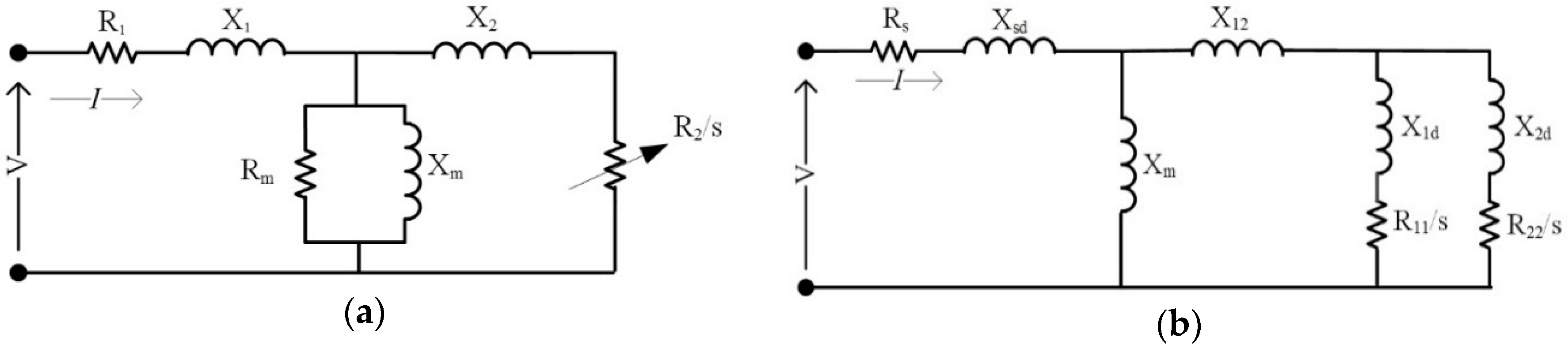
There are two basic IM models: single cage and double cage. In most papers, the IM is represented by using the single-cage model. However, the double-cage model is also popular especially for the representation of deep-bar machines [10,13,20,40]. However, apart from the predominantly used models, an IM is modeled by using a triple-cage model in [61]. The equivalent circuit of the single-cage model of the IM is presented in Figure 1a. In this figure, R₁, R₂, R_m, X₁, X₂, and X_m represent the stator resistance, rotor resistance in reference to stator side, core loss resistance, stator leakage reactance, rotor leakage reactance resistance in reference to stator side, and magnetizing reactance, respectively [4]. Therefore, in general, this circuit has six different parameters. However, in many papers dealing with induction machine parameter estimation, the value of the core loss resistance is ignored (for example in [18,26,51,65] and so on). The steady-state equivalent circuit of the double-cage IM, shown in Figure 1b, contains, in general, eight electrical parameters. In this circuit, parameters R_s and X_sd correspond to stator variables, while X₁₂, X_1d, X_2d, R₁₁, and R₂₂ correspond to rotor variables (one cage is represented by X_1d and R₁₁, while the second is defined with X_2d and R₂₂). The magnetizing part of the circuit is represented by X_m. However, in some papers dealing with the double-cage IM, the value of the stator reactance X_sd and/or the value of the mutual rotor reactance X₁₂ are ignored [5,13,20].

It is interesting to note that in [33,51] it is stated that the usage of a single-cage induction machine is neither an appropriate model nor sufficient for the prediction of the starting current. Namely, to predict the starting current, a double-cage induction machine model needs to be used. In the double-cage induction machine model, there exist two cages: an outer cage (whose effect is predominant near to zero speed) and an inner cage (whose effect is predominant near to rated speed) [1]. However, for estimation, the usage of the single cage machine model makes it possible to solve a system of equations with a maximum of six unknown parameters. On the other hand, if we use the double cage model, in the optimization process we have a maximum of eight unknown parameters, which increases the complexity of the problem.

3. Parameter Estimation Methods Based on Steady-State Models: An Overview

The methods for IM parameter estimation based on machine steady-state models can be divided into two main groups. The first group represents the usage of IEEE and IEC standards. The second group represents the usage of catalog/manufacturer/nameplate data or measured data for machine parameter estimation. As these methods are predominantly based on solving a system of equations, the attention in this section is given to the optimization techniques known from the literature, too.

3.1. IEEE and IEC standards

In IEEE Standard 112 [2], the IEEE Power Engineering Society recommends different methods for IM parameter estimation and calculations. Some of the IEEE recommended methods use data from no-load or locked-rotor tests with rated/non-rated frequencies (Methods 1 and 2), while others use data from no-load or full-load slip tests with reduced supply voltage (Methods 3 and 4). Furthermore, Method 1 requires a test at a maximum of 25% of rated frequency, while Method 2 requires tests for three different frequencies. On the other hand, Method 3 assumes that a test should be carried out with or without a coupled load, while Method 4 implies performing locked-rotor tests at rated frequency. Also, Methods 1, 2, and 4 require the implementation of tests at rated current, that is, precise current measurement, while Method 3 requires precise slip measurement.

Besides IEEE Standards, there is also an IEC standard for IM parameter determination [3]. The IEC Standard 60034-28 establishes procedures to obtain values for elements of single-phase equivalent circuit diagrams from tests and defines standard elements of these diagrams. Also, this standard gives the procedures for the determination of equivalent circuit parameters from a load curve test as an alternative to the reverse rotation and locked rotor tests. Therefore, it can be concluded that the IEEE and IEC standards for IM parameter determination are not easy to implement. Furthermore, they can be erroneous, which is specially mentioned in [5].

3.2. Methods Based on Catalog/Manufacturer/Nameplate Data

The IM nameplate provides very important data. However, different machine manufacturers give different data. On some machines, the nameplate can give only basic information about the machine, such as its rated voltage, power, and speed, while on others, the nameplate can also give some information related to torque data. However, technical (machine) documentation (catalog data or manufacturer data) for novel IMs gives a lot of information. For that reason, methods from this group published in the literature are based on the usage of different variables [5,13,18,20] (for example, rated and maximum torque, rated and maximum current, rated power, rated power factor, starting current, etc.). Hence, one can say that methods based on catalog/manufacturer/nameplate data are very appropriate for novel IMs that have full manufacturer data. However, they are not useful for old machines as they do not have catalog data or their catalog data do not contain detailed information. Furthermore, during long-term operation, the IMs changes its characteristics (magnetic material, isolation, eccentricity, etc.) and then these methods cannot be taken as a standard method for IM parameter estimation.

3.3. Methods Based on Measured Data

Methods based on measured data require certain measurements on the observed machine. For that reason, these methods are very reliable and reflect the actual condition of the machine. Furthermore, these methods are very effective for old IMs that do not have full catalog data. However, for their implementation, a precise sensor must be used. It was noted earlier that machine torque measurement is not needed for adequate machine representation [5]. However, to present a different load value, a speed measurement is required (except if we apply methods based on real-time parameter estimation, such as [71]). Therefore, methods based on measurements of phase speed, machine input power, machine torque, and current are presented in [12]. By using all these data, the authors presented a full machine model taking into account changes in parameters with speed. On the other hand, methods for IM parameter estimation based on phase current and power factor measurements at different speed values are described in [45,46]. Besides them, methods based on torque measurement also belong in this group [38].

3.4. Methods Based on Optimization Algorithms

The estimation of the IM parameters, regardless of whether they use the catalog, nameplate, manufacturer, or measured data, requires solving a large number of complex equations. The predefined equations can be solved analytically or by using iterative or optimization techniques. Analytical methods, such as the methods described in [10,11] as well as those based on open-circuit and short-circuit experiments, are very simple to implement. However, analytical methods require the introduction of appropriate assumptions or the usage of some approximative formulation. Therefore, these methods allow parameters to be obtained very quickly with low accuracy values. The most commonly used iterative techniques for IM parameter estimation are based on the usage of the well-known Newton-Raphson algorithm or the Levenberg-Marquardt algorithm [12,13]. For the implementation of these algorithms, certain assumptions or additional known data are required. Furthermore, for its implementation, it is necessary to accurately define the iteration step, starting values, and appropriate iteration criteria.

On the other hand, many papers dealing with IM parameter estimation are based on the usage of different optimization (usually metaheuristic) techniques [14,15,16,17,18,19,20,21,22,23,24,25,26,27,28,29,30,31,32,33,34,35,43]. The usage of optimization techniques requires solving of the equation to satisfy predefined criteria or an objective function. The IM parameters can be obtained by using the genetic algorithm (GA) [14,15,16,17,18,19,20,21,22,23,24], genetic programming (GP) [15], particle swarm optimization (PSO) algorithm [14,16,18,19,20,21,22,25,26,27,28,43], hybrid GA and PSO (HGAPSO) [18], simulated annealing (SA) [19,27], bacterial foraging technique (BFT) [26], shuffled frog-leaping algorithm (SFLA) [14,20], modified shuffled frog-leaping algorithm (MSFLA) [14], artificial bee colony (abc) algorithm [21], charged system search (CSS) [22], artificial fish swarm algorithm (AFSA) [23], simple random search (SRS) method [24], immune algorithm (IA) [17,26], steepest descent local search (SDLS) algorithm [27], evolution strategies (ESs) [27], simple evolutionary algorithm (SEA) [27], diversity-guided evolutionary algorithm (DGEA) [27], scatter search (SS) [28], ant colony algorithm (ACA) [28], sparse grid optimization algorithm (SGOA) [29], dynamic encoding (DEn) algorithm [30], vector constructing method (VCM) [32], least-squares algorithm (LSA) [33], mean-variance mapping optimization (MVMO) [34], and differential evolution (DE) algorithm [14,22,31,35].

Besides the abovementioned techniques and methods, neural networks can also be used for IM parameter determination [44]. However, the usage of neural networks requires a lot of data to train the algorithm. Also, these methods require a high-speed processor for data processing. However, most of these papers base their estimates on manufacturers’ data. Besides, no algorithm has yet proven its significant superiority in the problem under study. Furthermore, there is no paper where the authors test the proposed algorithm on a different kind of input data.

From the perspective of objective functions for IM parameter estimation, the problem of finding unknown machine parameters is reduced to the problem of minimization of the deviation between the measured, catalog, or manufacturer data and the estimated value of a certain variable or variables in papers that deal with the usage of optimization techniques for IM parameter estimation. The mentioned deviation is known as the objective function (OF) or fitness function. In the literature, there are many types of objective functions. Some of them require the value of active and reactive current components [29], instantaneous current value [27], power factor, RMS phase voltage and RMS phase current [5], torque, current and power factor values [20], torque and power factor values [18], current and torque value [45], power and torque values [13], and similar. Therefore, different combinations of used variables can be found in existing objective functions. However, it is interesting to note that the investigation presented in [5] strictly notes that the information about the power factor, RMS phase voltage, and RMS phase current is sufficient for IM parameter determination. Furthermore, the torque measurement is not required for IM parameter estimation. It is well known that torque sensors are high-price devices, and therefore the method described in [5] is very popular in science.

4. SA-ERWCA

A novel hybrid metaheuristic algorithm named SA-ERWCA is proposed in this work. The idea of merging the SA algorithm with population-based algorithms comes from many existing studies that propose hybridization of SA with EAs, as concisely presented in [81]. According to [81], the two categories of hybrid SA and EAs can be defined:

(i) Collaborative hybrid metaheuristics are based on the exchange of information between different self-contained metaheuristics and can be divided into two subcategories [82,83,84,85,86,87,88]:

• Teamwork collaborative algorithms are hybrids where both algorithms work in parallel [82,83,84,85].
• Relay collaborative algorithms rely on executing the algorithms one after another [86,87,88].

One such hybrid type is EA-SA, which is based on optimizing the use of EA and additionally improving the obtained optimal solution with the SA algorithm [86,87]. Another type of relay collaborative algorithm is SA-EA, in which SA is used to initialize the population of the EA [81,88].

(ii) In the case of the integrative hybrid metaheuristics, one algorithm (subordinate) is embedded into the other algorithm (master). Precisely, only a certain function or component of one algorithm is replaced by the other algorithm [89,90,91].

As was mentioned before, ERWCA is a population-based algorithm, which means the first step of this algorithm must be the initialization of the population. Assuming that the size of the population is N_pop and N is the number of design variables (or dimension of the problem), a population is a matrix with dimensions N_pop × N. In the original ERWCA, the population is initialized randomly between the upper bound (UB) and the lower bound (LB) of the design variables. In the hybrid SA-ERWCA proposed in this paper, the SA algorithm is used to initialize the population of the ERWCA, similarly to the relay-collaborative strategy presented in [81,88].

Each individual of the population is denoted as ${\overrightarrow{X}}_i,\forall i=1,2,\dots N_{pop}$ and represents a vector that has N elements. The initialization process employing the SA algorithm is precisely described with the pseudo-code (PC₀) given in

Table 1. Pseudo-code of the SA algorithm.

Pseudo-Code of the SA Algorithm (PC0)
For each individual ${\overrightarrow{X}}_i,\forall i=1,2,\dots N_{pop}$
Enter the input data: k = 0, ck = c0, Lk = L0
${\overrightarrow{X}}_i=rand\times (UB-LB)+LB$
Repeat
For l = 0 to Lk
Generate a solution ${\overrightarrow{X}}_j$ from the neighborhood of the current solution ${\overrightarrow{X}}_i$
If $OF({\overrightarrow{X}}_j)<OF({\overrightarrow{X}}_i)$ then ${\overrightarrow{X}}_j$ becomes the current solution $({\overrightarrow{X}}_i={\overrightarrow{X}}_j)$
Else ${\overrightarrow{X}}_j$ becomes the current solution with the probability $e^{\left(\frac{f({\overrightarrow{X}}_i)-f({\overrightarrow{X}}_j)}{c_k}\right)}$
k = k + 1
Compute Lk and ck
Until ck ≅ 0

.

The parameters of the SA algorithm, c_k and L_k, are the temperature and number of transitions generated at some iteration k. They are calculated as explained in [91]. Also, rand represents a vector of random numbers between 0 and 1. After the initialization process, the obtained population must be sorted according to the value of the fitness function of each individual. Namely, the best individual, which has the minimum fitness function value, is chosen to be the sea. Besides the sea, the population consists of rivers and streams. The predefined parameter of the ERWCA is denoted as N_r and represents the number of rivers. Thus, N_r individuals of the initial population with the minimum fitness function value (except the sea) are chosen to be the rivers. Finally, the rest of the population is considered as streams: N_streams = N_pop − N_sr, where N_sr stands for the number of rivers plus the sea (N_sr = N_r +1). According to the water cycle process in nature, each stream flows directly or indirectly to the rivers or sea. The number of streams for each river and sea is calculated as follows:

$$C_n=f({\overrightarrow{X}}_n)-f({\overrightarrow{X}}_{N_{sr}+1}),n=1,2,\dots ,N_{sr}$$

(1)

$$N{S}_n=\mathrm{round}\left\{\left|\frac{C_n}{{{\displaystyle \sum }}_{n=1}^{N_{sr}}{C}_n}\right|N_{streams}\right\},n=1,,2,\dots ,N_{sr}$$

(2)

where NS_n represents the number of streams that flow to the nth river (or the sea of n is equal to 1). Since it was highlighted that streams continue their flow to either other rivers or directly to the sea, the next step in the ERWCA is to mathematically model the flow of streams. To that end, two update equations for the position of streams that flow to rivers and the sea are given (3) and (4), respectively:

$${\overrightarrow{X}}_{stream}(t+1)={\overrightarrow{X}}_{stream}(t)+rand\times C\times \left({\overrightarrow{X}}_{river}(t)-{\overrightarrow{X}}_{stream}(t)\right)$$

(3)

$${\overrightarrow{X}}_{stream}(t+1)={\overrightarrow{X}}_{stream}(t)+rand\times C\times \left({\overrightarrow{X}}_{sea}(t)-{\overrightarrow{X}}_{stream}(t)\right)$$

(4)

where rand is a random number with the range [0, 1], C is a parameter whose selected value is 2, and t is the current iteration. After updating the positions of streams, it is necessary to check whether the solution obtained by the stream is better than that obtained by its connecting river. In other words, if the stream has a lower fitness function than the river, the positions of stream and river are switched (the stream becomes a river and the river becomes a stream). Similarly, to streams, the rivers also update their positions using (5), thus:

$${\overrightarrow{X}}_{river}(t+1)={\overrightarrow{X}}_{river}(t)+rand\times C\times \left({\overrightarrow{X}}_{sea}(t)-{\overrightarrow{X}}_{river}(t)\right)$$

(5)

If the following update equation provides a river whose fitness function value is lower compared to the sea, then an interchange between the sea and the river must be carried out.

To provide an escape from local optima, the evaporation concept is built into the algorithm. In nature, evaporation can happen in different cases. Firstly, if a certain river has only a few streams, it evaporates before it can reach the sea. This process is mathematically modeled by the evaporation rate (ER), which is defined for each river as follows:

$$ER=\frac{sum(N{S}_n)}{N_{sr}-1}\times rand,\forall n=2,3,\dots ,N_{sr}$$

(6)

Evaporation of the river is followed by the rain process, which contributes to the formation of a new stream:

$${\overrightarrow{X}}_{stream}^{new}(t+1)=LB+rand\times (UB-LB)$$

(7)

The whole evaporation process of the river is presented using the pseudo-code PC₁, presented in

Table 2. Pseudo-code of the whole evaporation process of the river.

Pseudo-Code (PC1)
for i = 1: Nsr − 1
If (exp(−t/tmax) < rand) & (NSi < ER)
Perform rain process represented by (7)
End for

, where t_max stands for the maximum number of iterations.

However, in this case, the evaporation process occurs when rivers or streams flow into the sea, causing seawater to evaporate. Before applying the evaporation process, it should be checked whether the rivers and streams are close enough to the sea to cause evaporation. Evaporation of the seawater in the case of a river flowing into the sea is modeled as presented by the pseudo-code PC₂, represented in

Table 3. Pseudo-code of the evaporation of the seawater.

Pseudo-Code (PC2)
If $|{\overrightarrow{X}}_{sea}-{\overrightarrow{X}}_{river}^i|<d_{max}$ or $rand<0.1,i=1,2,\dots N_{sr}-1$
Perform rain process represented by (7).

.

Similarly, to the presented model, the evaporation when the stream flows into the sea is modelled with the pseudo-code PC₃, presented in

Table 4. Pseudo-code of flow of the stream into the sea.

Pseudo-Code (PC3)
If $|{\overrightarrow{X}}_{sea}-{\overrightarrow{X}}_{stream}^i|<d_{max},i=1,2,\dots N{S}_1$
Perform rain process represented by (8).

.

The equation that describes the rain process in this case is:

$${\overrightarrow{X}}_{stream}^{new}(t+1)={\overrightarrow{X}}_{sea}(t)+\sqrt{\mu }\times randn(1,N)$$

(8)

where μ is a coefficient set as 0.1, randn(1, N) is a vector of N standard Gaussian numbers, and d_max is an adaptive parameter calculated as follows:

$$d_{max}(t+1)=d_{max}(t)-\frac{d_{max}(t)}{t_{max}}$$

(9)

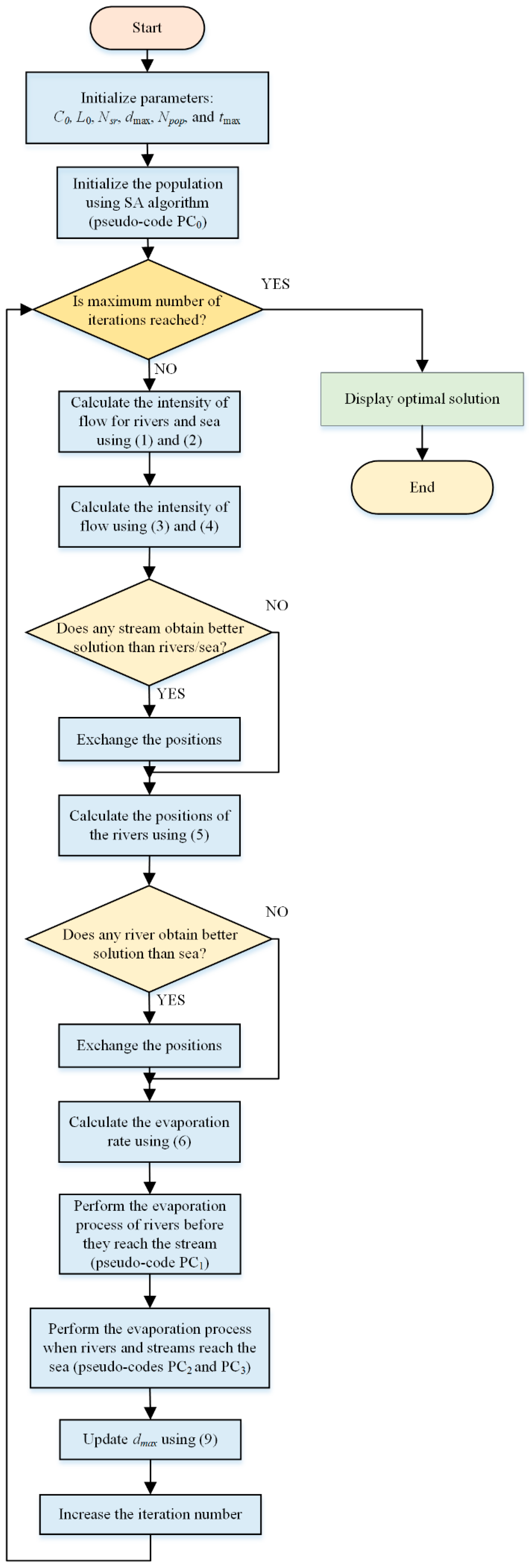
After the evaporation process finishes, one iteration of the SA-ERWCA is completed, and the process is repeated iteratively until the maximum number of iterations is reached. The complete pseudo-code (PC_SA-ERWCA) of the SA-ERWCA is presented in

Table 5. The complete pseudo-code of the SA-ERWCA.

Pseudo-Code (PCSA-ERWCA)
Enter the parameters: Nsr, dmax, Npop, and tmax
Initialize the population using the SA algorithm
t = 1
while (t < tmax)
Calculate the intensity of flow for rivers and sea using (1) and (2)
Calculate the positions of the streams using (3) and (4)
If a certain stream finds a better solution than the rivers/sea then exchange the positions
Calculate the positions of the rivers according to (5)
If a river obtains a better solution than the sea; then, exchange the positions
Calculate the evaporation rate ER as given by (6)
Check the evaporation condition among rivers and streams and calculate the new positions using PC1
Similarly, to the previous step, check the evaporation conditions between sea and streams/rivers and calculate new positions PC2 and PC3
Update the value of dmax using (9)
t = t + 1
End while

. Also, a flow chart of the SA-ERWCA is illustrated in Figure 2.

5. Simulation Results

First, we compared the SA-ERWCA with some competitive optimization techniques for 4 benchmark optimization problems, presented in

Table 6. Four benchmark test functions [92].

Function	Dimension	Range	fmin
$f_1={\displaystyle {\displaystyle \sum }_{i=1}^n}{x}_i^2$	n	[−100, 100]	0
$f_2={\displaystyle {\displaystyle \sum }_{i=1}^n}\left|x_i\right|+{\displaystyle {\displaystyle \prod }_{i=1}^n}|x_i|$	n	[−10, 10]	0
$f_3={\displaystyle {\displaystyle \sum }_{i=1}^n}{\left({\displaystyle {\displaystyle \sum }_{j-1}^i}{x}_j\right)}^2$	n	[−100, 100]	0
$f_4={\displaystyle {\displaystyle \sum }_{i=1}^{n-1}}[100(x_{i+1}-x_i^2)+{(x_i-1)}^2]$	n	[−30, 30]	0

. The optimization techniques used for comparison include moth-flame optimization (MFO), multi-verse optimization (MVO), PSO, and DEA [92,93]. The default parameters of these algorithms are used. The algorithms were executed under the same conditions to attain fairness in comparative experiments. Among them, the population was set to 30, the dimension (n) and the maximum iteration number was set to 30 and 1000, respectively. All the compared algorithms were run individually 30 times in each function and averaged as the final running result.

Further, standard deviation (STD), average results (AVG), and median (MED) were calculated to evaluate the results obtained to measure the experiment results.

Table 7. Comparison results of the 4 functions during 300,000 evaluations.

Functions	f1			f2
Algorithms	AVG	STD	MED	AVG	STD	MED
SA-ERWCA	1.12 × 10−10	7.80 × 10−11	9.01 × 10−11	3.88 × 10−4	2.9 × 10−4	2.6810−4
MFO	1670	3790	1667	35.3	24.5	35.3
MVO	3.11 × 10−3	7.04 × 10−4	596	3.84 × 10−2	1.3 × 10−2	11.13
PSO	101	14.3	111.3	46.9	3.54	51.56
DE	2.38 × 10−2	2.48 × 10−2	5.56 × 10−2	1.18 × 10−2	3.99 × 10−3	1.7 × 10−2
Functions	f3			f4
Algorithms	AVG	STD	MED	AVG	STD	MED
SA-ERWCA	0.3437	0.2297	0.3265	21.915	2.00	21.82
MFO	15,800	10,800	15,785	2.69 × 106	1.46 × 107	2.68 × 106
MVO	0.37	0.31	1613	66.8	94.5	3.59 × 104
PSO	185	27.6	220.5	8.98 × 104	1.83 × 104	1.08 × 105
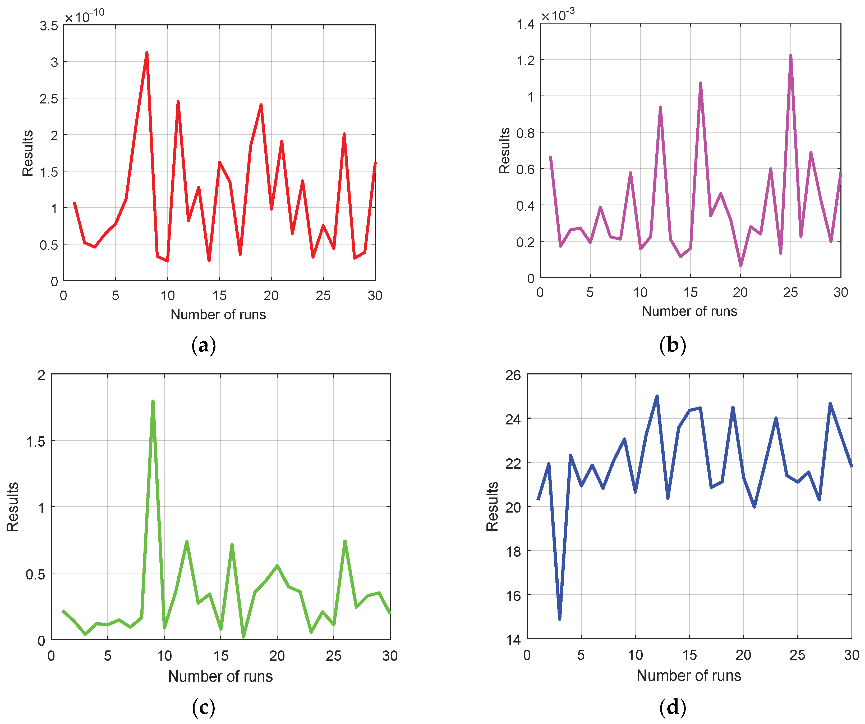
DE	1390	773	6275	30.8	18.1	32.59

presents the comparison results of the four functions during 300,000 evaluations. Also, Figure 3 shows the values of the OF for the four functions during the different runs. From Table 7, one can note that the AVG and MED values of the SA-ERWCA are better than those obtained using the other algorithms, which validate the effectiveness of the SA-ERWCA, even with the increased number of iterations during 300,000 evaluations.

Second, the application of SA-ERWCA for IM parameter estimation is presented. The application is tested on three different IMs based on their manufacturer data as well as on two IMs based on their measured data. All the considered machines are taken from the literature. However, it should be noted that for some machines we considered only a single-cage equivalent circuit (Machines 1, 4 and 5), while for others we considered a double-cage one (Machines 2 and 3). This is done to make a comparison with literature solutions.

For all simulation results, the population size was 200, while the maximum number of iterations was 150. Note that in all equations in this section the index “cal” represents the calculated value, the index “m” represents manufacturer data, and the index “mes” represents measured data. Also, mathematical equations for calculation of all machine variables are given in Appendix A for the single-cage machine (SCIM) and in Appendix B for the double-cage machine (DCIM).

5.1. Simulation Results for Machine 1

In [14], the authors proposed the usage of the SFLA for SCIM estimation based on manufacturer data presented in

Table 8. Data of Machine 1 [14].

Parameter	Value	Parameter	Value	Design Variables
Pn	40 HP	Tfl	190	$0.1\le R_1\le 0.6$
V	400 V	Tmax	370	$0.2\le R_2\le 0.6$
f	50 Hz	pffl	0.8	$0.1\le X_1\le 0.5$
p	2	sfl	0.09	$0.3\le X_2\le 1.0$
Tst	260			$4\le X_m\le 11$

. Also, they compared the obtained parameter values, as well as the machine characteristics, with the corresponding results obtained by using DE, PSO, and GA. The circuit parameters are found as the result of the error minimization function between the estimated and manufacturer data. In [14] the following OF is used:

$$OF=F_1^2+F_2^2+F_3^2+F_4^2$$

(10)

so that:

$$F_1=\frac{T_{fl,cal}-T_{fl,m}}{T_{fl,m}}$$

(11)

$$F_2=\frac{T_{st,cal}-T_{st,m}}{T_{st,m}}$$

(12)

$$F_3=\frac{T_{max,cal}-T_{max,m}}{T_{max,m}}$$

(13)

$$F_4=\frac{p{f}_{fl,cal}-p{f}_{fl,m}}{p{f}_{fl,m}}$$

(14)

The proposed SA-ERWCA technique is applied for parameter estimation of Machine 1, considering the parameter range given in Table 8.

A comparative study with SFLA, DE, GA, PSO, and MSFLA was done to validate the performance of the proposed algorithm, as presented in

Table 9. Results obtained for Machine 1.

Parameter (Ω)	DE [14]	GA [14]	PSO [14]	SFLA [14]	MSFLA [14]	SA-ERWCA
R1	0.4993	0.4875	0.3555	0.3437	0.270719	0.27821
X1	0.3264	0.3264	0.3455	0.3360	0.357274	0.20111
R2	0.3510	0.3556	0.4353	0.4345	0.477311	0.38795
X2	0.3510	0.3556	0.4353	0.4345	0.477311	0.80380
Xm	5.6967	6.6072	6.4223	6.2629	7.543194	7.87820

and

Table 10. Comparisons of results.

Manufacturer Data	DE		GA		PSO
	Value	$\left|\mathit{e}\right|$	Value	$\left|\mathit{e}\right|$	Value	$\left|\mathit{e}\right|$
Tfl	190.902	0.902	192.788	2.788	190.453	0.453
Tst	265.669	5.669	268.016	8.016	263.337	3.337
Tmax	349.842	20.158	354.092	15.908	363.730	6.27
pffl	0.8065	0.0065	0.817	0.017	0.7883	0.0117
OF	3.5 × 10−3		3.5 × 10−3		6.6 × 10−4
Manufacturer Data	SFLA		MSFLA		SA-ERWCA
	Value	$\left|\mathit{e}\right|$	Value	$\left|\mathit{e}\right|$	Value	$\left|\mathit{e}\right|$
Tfl	195.106	5.106	192.197	2.197	190.001	0.001
Tst	262.467	2.467	261.687	1.687	260.002	0.002
Tmax	368.036	1.964	373.852	3.852	370.000	0.0004
pffl	0.7860	0.014	0.7995	0.0005	0.8	0.0000
OF	1.1 × 10−3		2.8 × 10−4		1.6 × 10−10

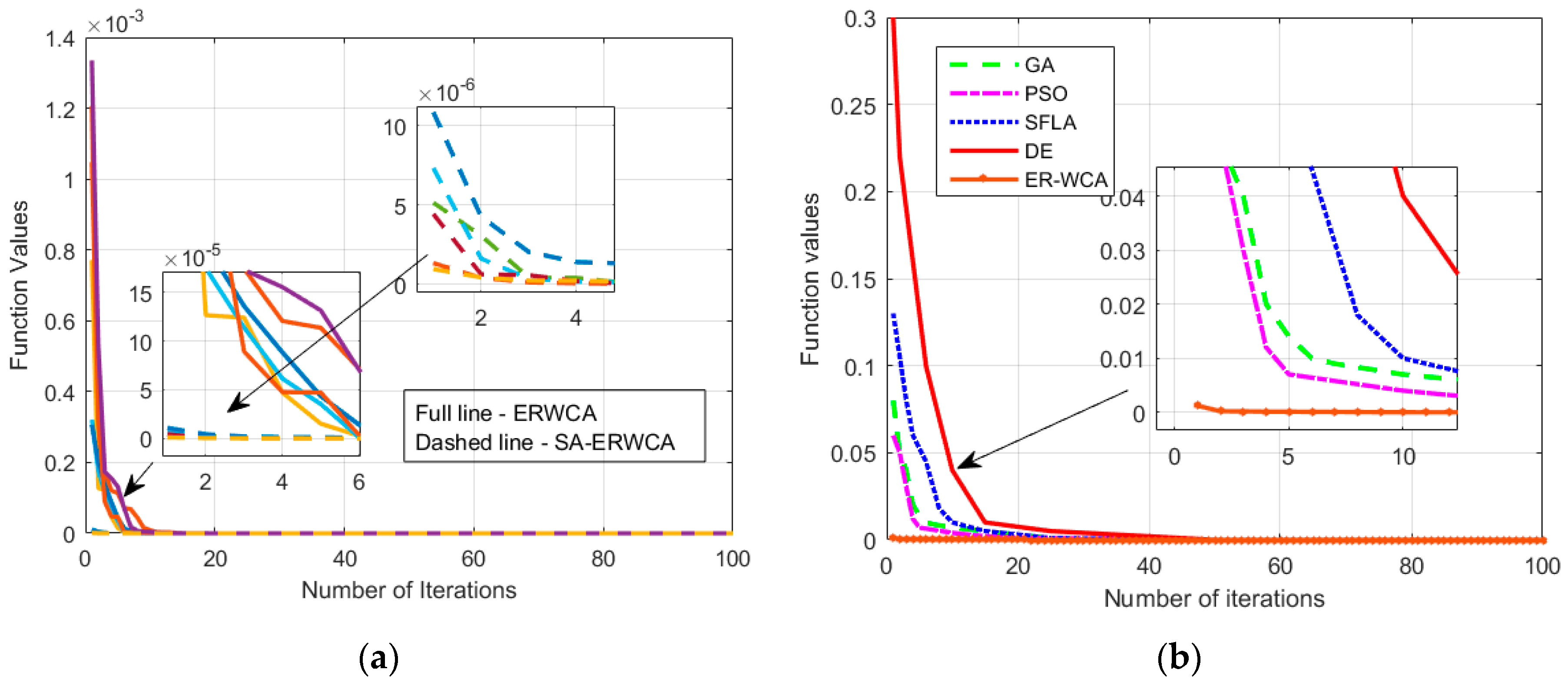
. It can be seen that SA-ERWCA gives better results than SFLA, DE, GA, PSO, and MSFLA. Furthermore, the value of the OF given in bold in Table 10 is considerably smaller with the proposed SA-ERWCA. It is very clear that SA-ERWCA obtains better convergence characteristics; the convergence characteristics of SA-ERWCA are much better for an initial number of iterations.

In the case, when we use SA-ERWCA, for a few starting iterations, the OF value is more than 10–15 times better in comparison with the classic ERWCA. For a higher number of iterations, the values of the objective function obtained by using SA-ERWCA are equal to or better than the corresponding curves obtained using ERWCA.

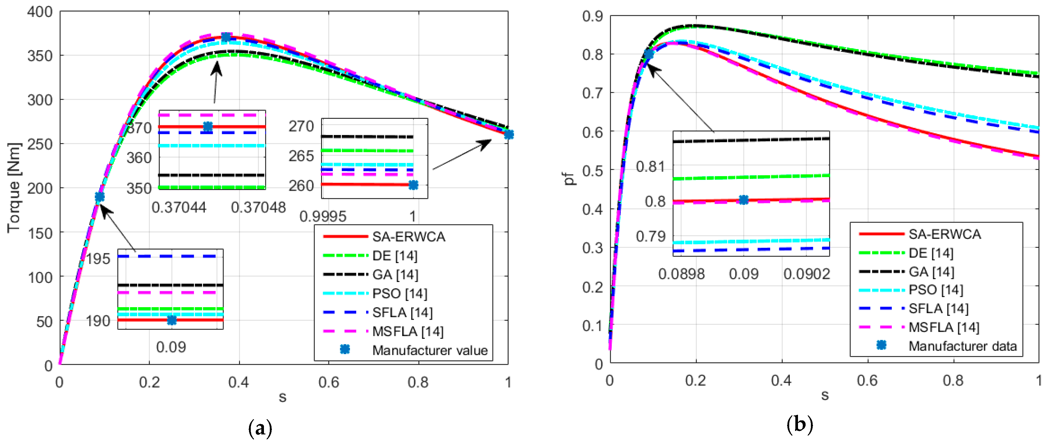
Figure 4 shows a comparison of the curves of the torque and power factor, respectively, obtained with SA-ERWCA, DE, GA, PSO, SFLA, and MSFLA. It can also be seen in this figure that the SA-ERWCA results for all of the slip zones are in good agreement with the manufacturer values. Figure 5a compares the mean values of the best six objective functions versus the number of iterations for ERWCA and SA-ERWCA when 100 simulation runs are performed.

The comparison of convergence characteristics between different algorithms is presented in Figure 5b. This figure shows that SA-ERWCA converges rapidly and reaches better results than the rest of the algorithms.

5.2. Simulation Results for Machine 2

In [20], the authors proposed the usage of PAMP and MSFLA for DCIM parameter estimation based on manufacturer data. For parameter estimation, the authors used the manufacturer data given in

Table 11. Data of Machine 2 [20].

Parameter	Value	Parameter	Value	Design Variables
Pn	148 HP	Tmax	1094.3 N	$0.02\le R_s\le 0.06$
V	400 V	pffl	0.9	$0.03\le X_{sd}\le 0.09$
f	50 Hz	sfl	0.0077	$2\le X_m\le 5$
p	2	Ist	1527.2 A	$0.005\le R_{11}\le 0.030$
Tst	847.2 N	Ifl	184 A	$0.05\le R_{22}\le 0.2$
Tfl	353 N			$0.1\le X_{1d}\le 0.2$ $0.04\le X_{2d}\le 0.20$

. In this case, the OF is as follows:

$$OF=F_1^2+F_2^2+F_3^2+F_4^2+F_5^2+F_6^2$$

(15)

so that:

$$F_1=\frac{T_{fl,cal}-T_{fl,m}}{T_{fl,m}}$$

(16)

$$F_2=\frac{T_{st,cal}-T_{st,m}}{T_{st,m}}$$

(17)

$$F_3=\frac{T_{max,cal}-T_{max,m}}{T_{max,m}}$$

(18)

$$F_4=\frac{p{f}_{fl,cal}-p{f}_{fl,m}}{p{f}_{fl,m}}$$

(19)

$$F_5=\frac{I_{st,cal}-I_{st,m}}{I_{st,m}}$$

(20)

$$F_6=\frac{I_{fl,cal}-I_{fl,m}}{I_{fl,m}}$$

(21)

A comparative study with PAMP and MSFLA was done to verify the effectiveness of the proposed algorithm (as shown in

Table 12. Results for PAMP, MSFLA and SA-ERWCA for Machine 2.

Parameter (Ω)	PAMP	MSFLA	SA-ERWCA
Rs	0.0375	0.0377	0.037614
Xsd	0.0692	0.0691	0.050454
Xm	3.7385	3.7475	3.767293
R11	0.0109	0.0109	0.010833
R22	0.1031	0.1032	0.135273
X1d	0.1424	0.1422	0.159068
X2d	0.0692	0.0691	0.112364

and

Table 13. Comparison of results with manufacturer data for Machine 2.

Manufacturer Data	MSFLA		PAMP		SA-ERWCA
	Value	$\left|\mathit{e}\right|$	Value	$\left|\mathit{e}\right|$	Value	$\left|\mathit{e}\right|$
Tfl	355.306	2.306	355.373	2.373	353.007	0.007
Tst	847.169	0.031	846.924	0.276	847.199	0.001
Tmax	1094.230	0.77	1094.112	0.288	094.315	0.015
pffl	0.9005	0.0005	0.9001	0.0001	0.8999	0.0001
Ifl	185.216	1.216	185.130	1.13	183.99	0.01
Ist	1527.262	0.062	1527.225	0.025	1527.196	0.004
OF	8.07 × 10−5		8.90 × 10−5		4.73 × 10−9

), in which it is evident that SA-ERWCA gives better results than PAMP and MSFLA and therefore fits the manufacturer data better.

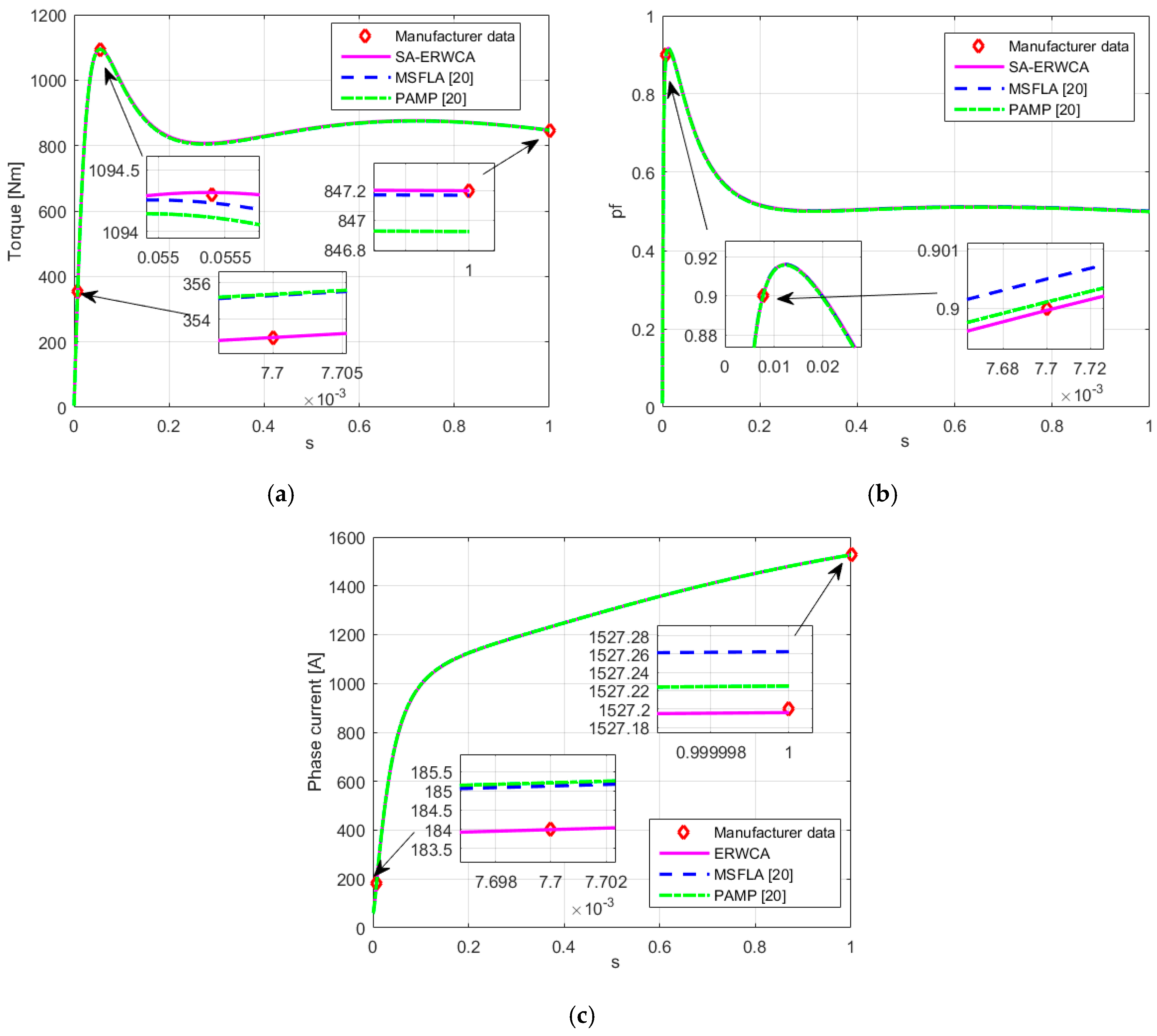
A comparison of the curves of the torque, power factor, and machine current, respectively, obtained by SA-ERWCA, PAMP and MSFLA is presented in Figure 6. It can be seen that the results of SA-ERWCA for all of the slip zones are in very good agreement with the manufacturer values. Also, its superiority over other considered algorithms is very evident.

5.3. Simulation Results for Machine 3

In [64], the authors proposed the usage of the instantaneous power of a free acceleration test for IM double-cage motor parameter estimation, in which, the authors compared the obtained results with the corresponding values of measured and manufacturer data presented in

Table 14. Data of Machine 3 [64].

Parameter	Value	Parameter	Value
Pn	75 HP	nr	1480 rpm
V	400 V	Tmax/Tfl	4.7
f	50 Hz	Tst/Tfl	3.8
p	2	Ist/Ifl	5.9

. Further, we have used the proposed algorithm, machine manufacturer data, and the following function.

$$OF=F_1^2+F_2^2+F_3^2$$

(22)

so that:

$$F_1=\frac{I_{st,m}}{I_{fl,m}}-\frac{I_{st,cal}}{I_{fl,cal}}$$

(23)

$$F_2=\frac{T_{st,m}}{T_{fl,m}}-\frac{T_{st,cal}}{T_{fl,cal}}$$

(24)

$$F_3=\frac{T_{max,m}}{T_{fl,m}}-\frac{T_{max,cal}}{T_{fl,cal}}$$

(25)

The obtained results are presented in

Table 15. Results for acceleration test and SA-ERWCA for Machine 3.

Parameter (Ω)	Acceleration Test	SA-ERWCA
Rs	0.11691	0.10001
Xsd	0.10688	0.15559
Xm	3.2023	5.1957
R11	0.03904	0.04089
R22	0.38144	0.29293
X1d	0.23872	0.21717
X2d	0.10688	0.01001

. In this table, the results obtained using an acceleration test are presented, too. The comparison of the results in terms of absolute error with manufacturer data is given in

Table 16. Comparison of acceleration test and SA-ERWCA results with manufacturer data for Machine 3.

Marked Data	Value	Acceleration Test		SA-ERWCA
		Value	$\left|\mathit{e}\right|$	Value	$\left|\mathit{e}\right|$
Tmax/Tfl	4.7	4.556	0.144	4.644	0.056
Tst/Tfl	3.8	3.529	0.271	3.788	0.012
Ist/Ifl	5.9	6.175	0.275	5.86	0.04
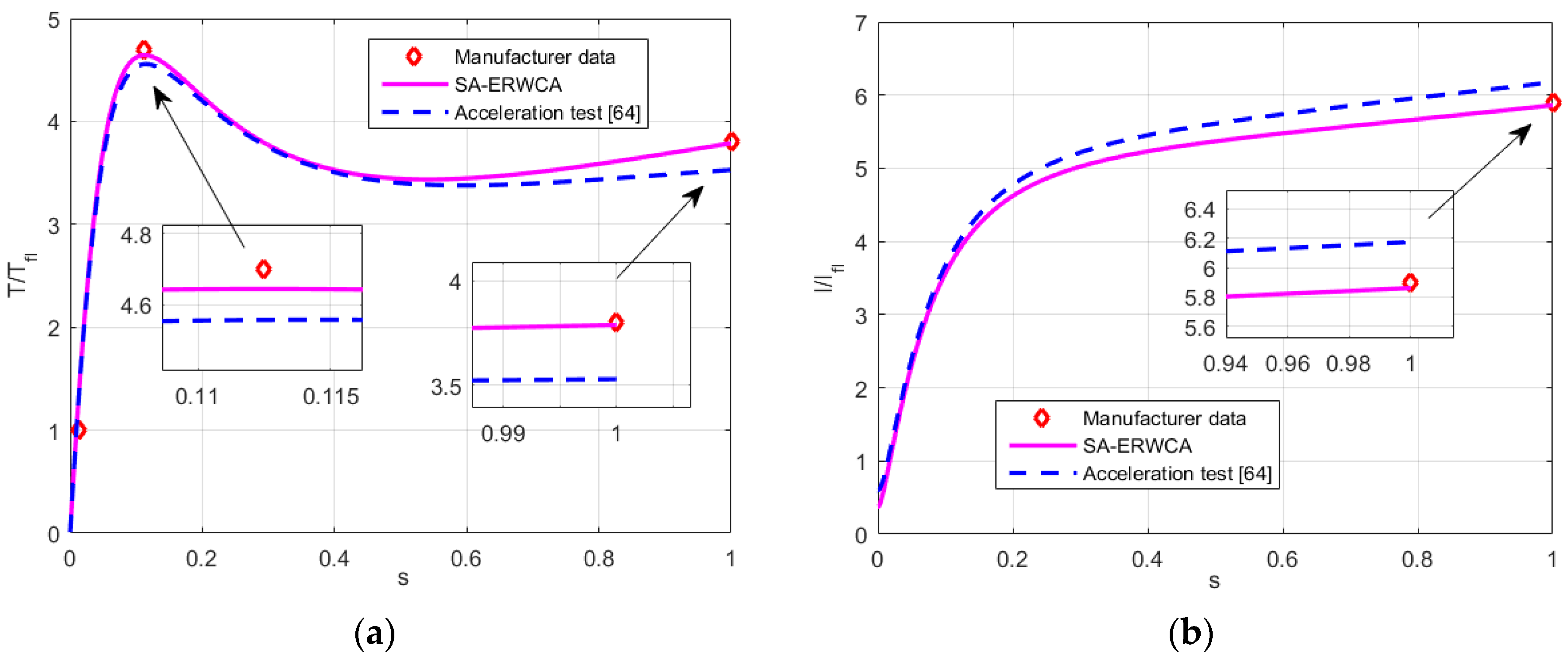
OF		0.1698		0.00488

. The errors obtained with the proposed algorithm are smaller than those obtained with the acceleration test. The same conclusion can be derived by considering the torque versus slip and phase current versus slip characteristics, presented in Figure 7.

5.4. Simulation Results for Machine 4

In [45], the authors proposed the usage of a GA for a SCIM parameter estimation based on measured data. The measured values of machine slip, current, and power factor are given in

Table 17. Data of Machine 4 and measured data: three-phase induction motor [45].

Parameter	Value	Measured Data
Pn	0.75 kW	Slip	Stator current (A)	Power factor
V	380 V	0.06	1.86	0.62
f	50 Hz	0.10	2.39	0.74
p	1	0.15	3.07	0.78

.

The circuit parameters are found as the result of the error minimization function between the estimated and measured data. In [45] the following OF is used:

$$OF={\displaystyle \sum }_{i=1}^n{\left(\frac{p{f}_{cal,i}}{p{f}_{meas,i}}-1\right)}^2+{\displaystyle \sum }_{i=1}^n{\left(\frac{I_{cal,i}}{I_{meas,i}}-1\right)}^2$$

(26)

where i represents the measured point (in this case n = 3, while i = 1, 2, and 3).

Table 18. Results for GA and SA-ERWCA for Machine 4.

Parameter (Ω)	GA [45]	SA-ERWCA
R1	10.28	10.094
X1	8.19	9.506
R2	10.48	10.238
X2	19.21	17.315
Xm	143.17	141.961

presents the results obtained using the proposed SA-ERWCA technique as well as the GA from [45]. For SA-ERWCA, ranges of the considered parameters are: $5\le R_1,X_1,R_2\le 15,10\le X_2\le 25,\mathrm{and}100\le X_m\le 180$.

The comparisons of GA and SA-ERWCA results with measured data are presented in

Table 19. Comparison of GA and SA-ERWCA results with measured data for Machine 4.

Slip	Measured Data	GA [45]		SA-ERWCA
	Stator Current(A)	Value	$\left|\mathit{e}\right|$	Value	$\left|\mathit{e}\right|$
0.06	1.86	1.8554	0.0046	1.8591	0.0009
0.10	2.39	2.3840	0.006	2.3921	0.0021
0.15	3.07	3.0542	0.0158	3.0685	0.0015
Slip	Measured Data	GA [45]		SA-ERWCA
	Power Factor	Value	$\left|\mathit{e}\right|$	Value	$\left|\mathit{e}\right|$
0.06	0.62	0.6193	0.0007	0.6203	0.0003
0.10	0.74	0.7366	0.0034	0.7375	0.0015
0.15	0.78	0.7812	−0.0012	0.7819	0.0019
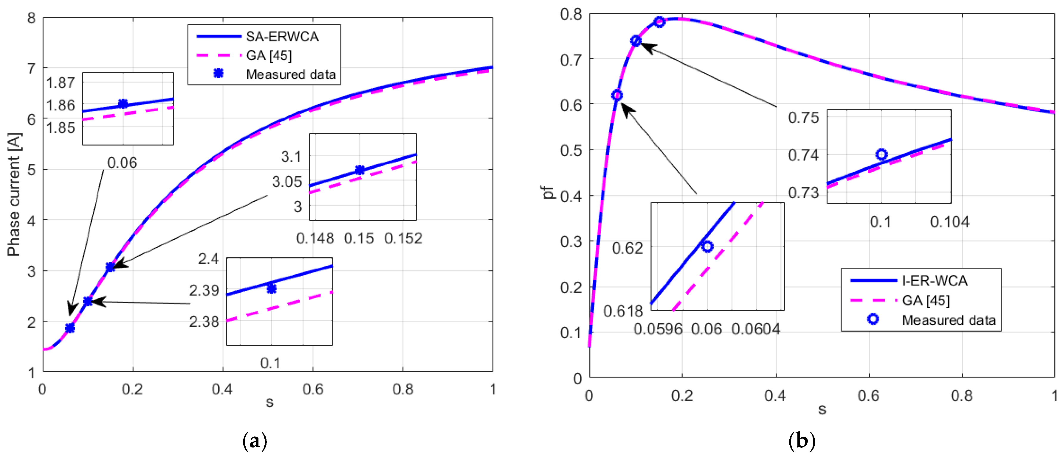
OF		2.18 × 10−4		2.31 × 10−5

. The comparison of the corresponding phase current versus slip and power factor versus slip characteristics is presented in Figure 8. It is clear that SA-ERWCA has better results than GA. Also, the value of the OF is smaller with the proposed SA-ERWCA.

5.5. Simulation Results for Machine 5

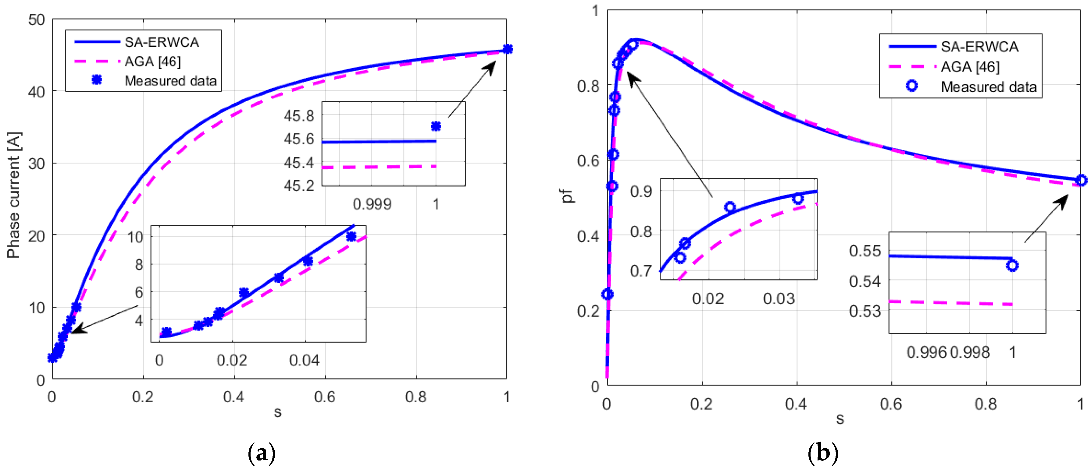
In [46], the authors proposed the usage of the new adaptive GA (AGA) for SCIM (with data presented in

Table 20. Data of Machine 5 [46].

Parameter	Value
Pn	4 kW
V	Δ/Y 220/380
Ifl	Δ/Y 14.2/8.2 A
pffl	0.88
nr	2870

) parameter estimation based on measured data. In which Machine 5 is a three-phase squirrel cage induction motor ELPROM, Type A0-112 M-2B3T-11. The measured values of machine speed, current, and power factor are given in

Table 21. Measured results from [46].

Speed (rpm)	Stator Current (A)	Angle (degree)	Power Factor
0	45.70	57.0	0.5446
2842	10.00	25.0	0.9063
2878	8.20	27.0	0.8910
2902	7.00	28.5	0.8788
2931	5.90	31.0	0.8572
2950	4.55	40.0	0.7660
2952	4.25	43.0	0.7314
2960	3.80	52.0	0.6157
2968	3.55	58.0	0.5299
2994	3.05	76.0	0.2419

.

To obtain the unknown values of parameters, the authors used the measured phase current value and its power factor, and the same OF given in (26). The results are presented in

Table 22. Results for AGA and SA-ERWCA for Machine 5.

Parameter (Ω)	AGA [46]	SA-ERWCA
R1	1.4460	1.6794
X1	2.0735	1.1164
R2	1.1994	1.0372
X2	2.0735	3.0241
Xm	72.728	78.723

and

Table 23. Comparison of AGA and SA-ERWCA results with measured data for Machine 5.

Speed (rpm)	Stator Current (A)		AGA [46]		SA-ERWCA
			Value	$\left|\mathit{e}\right|$	Value	$\left|\mathit{e}\right|$
0	45.7		45.3571	0.3429	45.5731	0.1269
2842	10		9.3893	0.6107	10.6616	0.6616
2878	8.2		7.5945	0.6055	8.5931	0.3931
2902	7.0		6.3968	0.6032	7.1816	0.1816
2931	5.9		4.9958	0.9042	5.4826	0.4174
2950	4.55		4.1558	0.3942	4.4225	0.1275
2952	4.25		4.0738	0.1762	4.3165	0.0665
2960	3.80		3.7634	0.0366	3.9089	0.1089
2968	3.55		3.4871	0.0629	3.5366	0.0134
2994	3.05		2.9566	0.0934	2.7801	0.2699
Speed (rpm)	Angle (degree)	Power Factor	AGA [46]		SA-ERWCA
			Value	$\left|\mathit{e}\right|$	Value	$\left|\mathit{e}\right|$
0	57	0.5446	0.5318	0.0128	0.5471	0.0025
2842	25	0.9063	0.9026	0.0037	0.9179	0.0116
2878	27	0.8910	0.8829	0.0081	0.9075	0.0165
2902	28.5	0.8788	0.8553	0.0235	0.8900	0.0112
2931	31	0.8572	0.7861	0.0711	0.8409	0.0163
2950	40	0.7660	0.6947	0.0713	0.7683	0.0023
2952	43	0.7314	0.6815	0.0499	0.7571	0.0257
2960	52	0.6157	0.6194	0.0037	0.7025	0.0868
2968	58	0.5299	0.5398	0.0099	0.6273	0.0974
2994	76	0.2419	0.1361	0.1058	0.1686	0.0733
OF			0.4667		0.2582

.

Visualization of the results obtained is shown in Figure 9 to declare that the SA-ERWCA obtains results that better fit the measured results, which demonstrate the applicability, efficiency, and accuracy of the proposed estimation technique for different IMs (different in respect to power value), different objective functions, and different kinds of input data.

6. Experimental Results

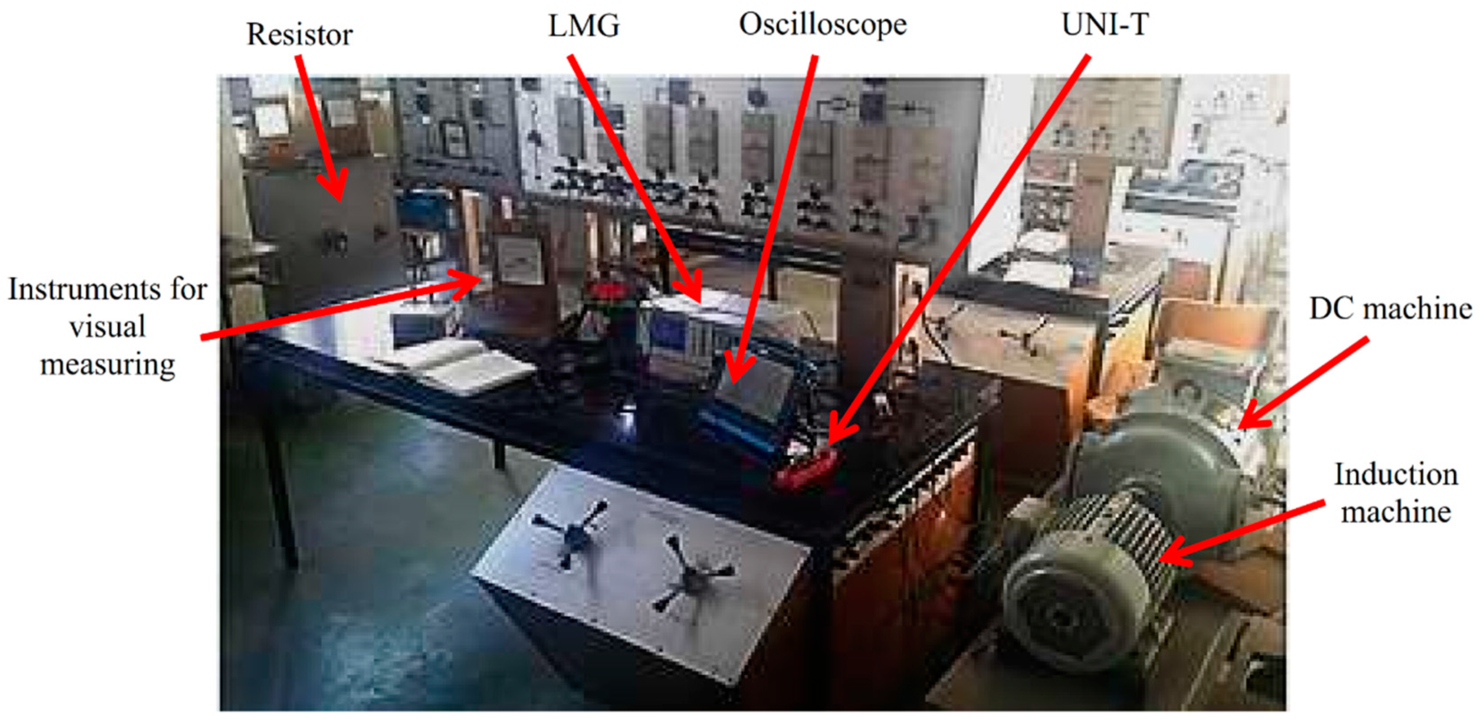
The verification of the applicability of SA-ERWCA for the IM parameter estimation is demonstrated by considering a 4-kW three-phase IM from the Laboratory for Electrical Machines and Drives at the Faculty of Electrical Engineering (University of Montenegro), shown in Figure 10. The bench used for obtaining the experimental data (phase current versus slip, power factor versus slip, input power versus slip, and reactive power versus slip characteristics) is composed of an IM (KONCAR, 4 kW, 380 V, 8.6 A, 1435 rpm, pf = 0.83) coupled to a DC motor/generator (KONCAR 230 V, 22.2 A, 5.1 A, 1450 rpm).

The DC machine is used as generator or motor. Namely, it is used to vary the slip of the IM over the negative (generator) and positive (motor) slip range. For the DC generator, the output is connected to a variable resistor. Active power, reactive power, voltage, and current are measured with an LMG power analyzer (Leistungsmessgerät). The speed is measured by using a UT372 speed sensor (UNI-T, Dongguan City, China), while the instantaneous value of the phase current and voltage are measured by using a TO102 oscilloscope (Shenzhen Micsig Instruments CO, Shenzhen, China) to check the RMS value of the phase current and voltage.

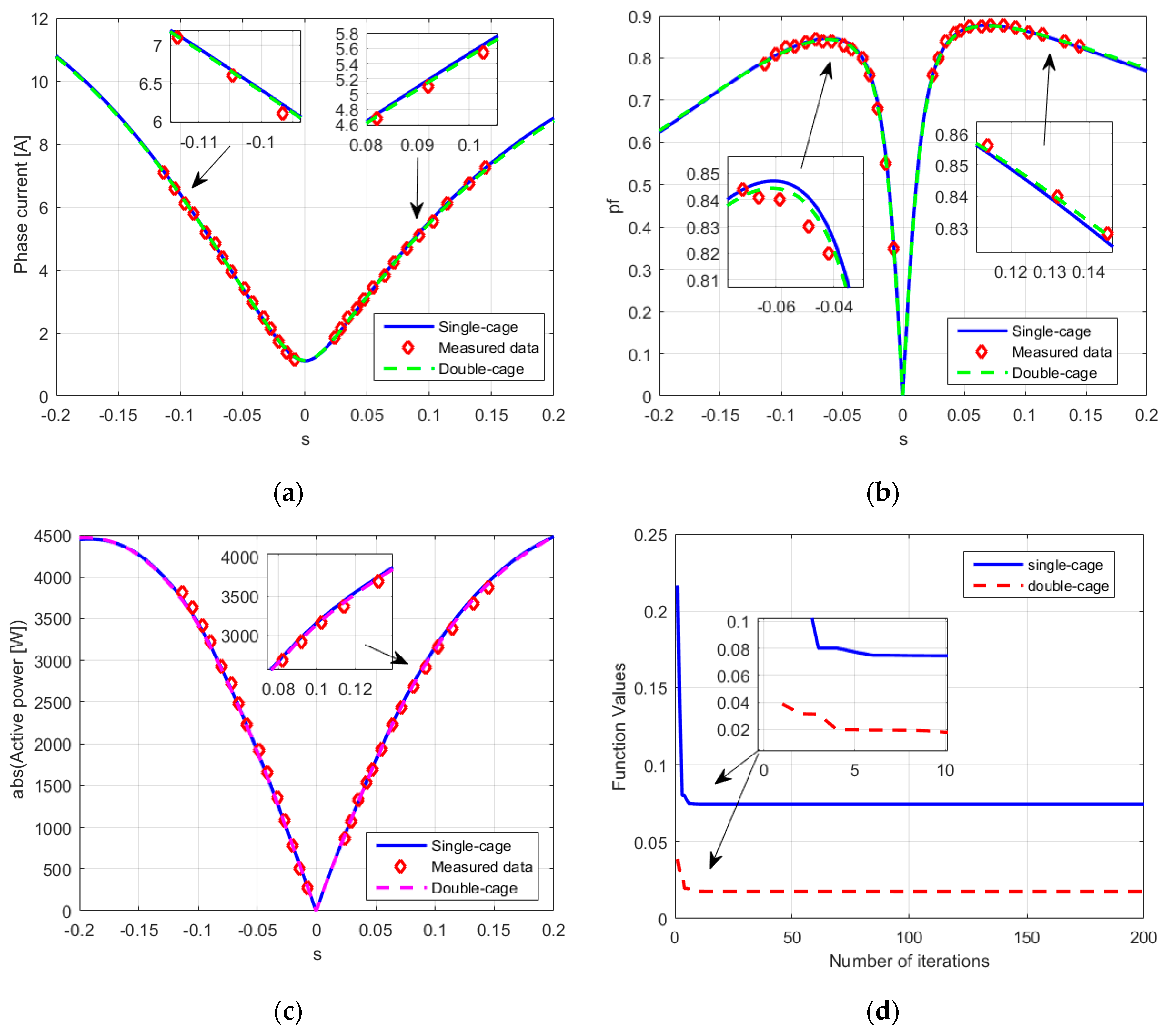
The measured phase current versus slip, power factor versus slip, and input power versus slip characteristics are shown in Figure 11. By using the obtained results and applying the proposed method and OF given in (26), the IM parameters were determined (as shown in

Table 24. Estimated IM parameters: Experimental Application.

Parameter (Ω)	Single Cage	Parameter (Ω)	Double Cage
R1	3.2342	Rs	3.3486
R2	3.5253	Xsd	0.1004
X1	5.7459	Xm	195.486
X2	9.2029	R11	4.5219
Xm	192.2646	R22	21.9186
		X1d	20.2025
		X2d	59.8289
OF		Single cage	0.0744
		Double cage	0.0178

) for both single-cage and double-cage equivalent circuits.

The calculated phase current versus slip, power factor versus slip, input power versus slip for the obtained machine parameters are also shown in Figure 11.

As can be seen, the calculated characteristics correspond very well with the measured characteristics. However, from the presented results and by observing the value of the calculated objective function, it is very clear that the double-cage model gives a better fit with the experimental results. Also, the proposed method guarantees that an optimal solution will be found quickly (as illustrated in Figure 11d). For the analyzed case, the accuracy of the obtained results is appropriate after only a few iterations.

7. Conclusions

An IM is the most frequently used type of electrical machine in industry. However, for accurate and precise IM dynamic simulations, an exact knowledge of its equivalent circuit parameters is required. In this paper, an overview of IM parameter estimation methods is given. Special attention is given to methods based on measured or nameplate/catalog/manufacturer data. The main part of the paper is devoted to the novel algorithm, called SA-ERWCA. The applicability of the proposed algorithm is tested by considering five different induction machines found in the literature. Furthermore, the considered machines have a wide power range. Also, the tests are realized using different objective functions, as well as for two equivalent machine circuits. Also, we compared the SA-ERWCA with some competitive optimization techniques for 4 benchmark optimization problems used in the literature. The obtained results demonstrate that the proposed algorithm enables better fitting between the measured (or marked) and simulated results than other methods used in the literature. Furthermore, the proposed algorithm has a very good convergence characteristic as it only reaches an appropriate level of accuracy after only a few iterations.

Besides, the paper also presents the results of the estimation for a laboratory 4-kW machine. In this case, the estimation is realized for both equivalent circuits. All results demonstrate the effectiveness and applicability of the proposed algorithm for IM parameter estimation. In future work, we will consider parameter estimation of IMs with variable parameters, as well as optimal design of other electromagnetic machines. Also, we will compare constant and variable machine parameter models.

References

1. Kazmierkowski, M.P. Electric Motor Drives: Modeling, Analysis and Control; Krishan, R., Ed.; Prentice-Hall: Upper Saddle River, NJ, USA, 2001. [Google Scholar]
2. IEEE Standard 112. Test Procedure for Polyphase Induction Motors and Generators; IEEE: New York City, NJ, USA, 2004. [Google Scholar]
3. IEC Standards 60034-28, Rotating Electrical Machines–Part 28: Test Methods for Determining Quantities of Equivalent Circuit Diagrams for Three-Phase Low-Voltage Cage Induction Motors; IEC: Geneva, Switzerland, 2012.
4. Al-Badri, M.; Pillay, P.; Angers, P. A Novel In Situ Efficiency Estimation Algorithm for Three-Phase IM Using GA, IEEE Method F1 Calculations, and Pretested Motor Data. IEEE Trans. Energy Convers. 2015, 30, 1092–1102. [Google Scholar] [CrossRef]
5. Pedra, J.; Sainz, L. Parameter estimation of squirrel-cage induction motors without torque measurements. IEEE Proc. Electr. Power Appl. 2006, 153, 263–270. [Google Scholar] [CrossRef]
6. Toliyat, H.A.; Levi, E.; Raina, M. A review of RFO induction motor parameter estimation techniques. IEEE Trans. Energy Convers. 2003, 18, 271–283. [Google Scholar] [CrossRef]
7. Lindenmeyer, D.; Dommel, H.W.; Moshref, A.; Kundur, P. An induction motor parameter estimation method. Int. J. Electr. Power Energy Syst. 2001, 23, 251–262. [Google Scholar] [CrossRef]
8. Tang, J.; Yang, Y.; Blaabjerg, F.; Chen, J.; Diao, L.; Liu, Z. Parameter Identification of Inverter-Fed Induction Motors: A Review. Energies 2018, 11, 2194. [Google Scholar] [CrossRef] [Green Version]
9. Odhano, S.A.; Pescetto, P.; Awan, H.A.; Hinkkanen, M.; Pellegrino, G.; Bojoi, R. Parameter Identification and Self-Commissioning in AC Motor Drives: A Technology Status Review. IEEE Trans. Power Electron. 2019, 34, 3603–3614. [Google Scholar] [CrossRef] [Green Version]
10. Yamamoto, S.; Hirahara, H.; Tanaka, A.; Ara, T. A simple method to determine double-cage rotor equivalent circuit parameters of induction motors from no-load and locked-rotor tests. IEEE Trans. Ind. Appl. 2019, 55, 273–282. [Google Scholar] [CrossRef]
11. Natarajan, R.; Misra, V.K. Parameter estimation of induction motors using a spreadsheet program on a personal computer. Electr. Power Syst. Res. 1989, 16, 157–164. [Google Scholar] [CrossRef]
12. Akbaba, M.; Taleb, M.; Rumeli, A. Improved estimation of induction machine parameters. Electr. Power Syst. Res. 1995, 34, 65–73. [Google Scholar] [CrossRef]
13. Haque, M.H. Determination of NEMA Design Induction Motor Parameters from Manufacturer Data. IEEE Trans. Energy Convers. 2008, 23, 997–1004. [Google Scholar] [CrossRef]
14. Perez, I.; Gomez-Gonzalez, M.; Jurado, F. Estimation of induction motor parameters using shuffled frog-leaping algorithm. Electr. Eng. 2013, 95, 267–275. [Google Scholar] [CrossRef]
15. Nangsue, P.; Pillay, P.; Conry, S.E. Evolutionary algorithms for induction motor parameter determination. IEEE Trans. Energy Convers. 1999, 14, 447–453. [Google Scholar] [CrossRef]
16. Sakthivel, V.; Bhuvaneswari, R.; Subramanian, S. Multi-objective parameter estimation of induction motor using particle swarm optimization. Eng. Appl. Artif. Intell. 2010, 23, 302–312. [Google Scholar] [CrossRef]
17. Sakthivel, V.; Bhuvaneswari, R.; Subramanian, S. Artificial immune system for parameter estimation of induction motor. Expert Syst. Appl. 2010, 37, 6109–6115. [Google Scholar] [CrossRef]
18. Mohammadi, H.R.; Akhavan, A. Parameter Estimation of Three-Phase Induction Motor Using Hybrid of Genetic Algorithm and Particle Swarm Optimization. J. Eng. 2014, 2014, 148204. [Google Scholar] [CrossRef] [Green Version]
19. Nikranajbar, A.; Ebrahimi, M.K.; Wood, A.S. Parameter identification of a cage induction motor using particle swarm optimization. Proc. Inst. Mech. Eng. Part I J. Syst. Control Eng. 2010, 224, 479–491. [Google Scholar] [CrossRef] [Green Version]
20. Gomez-Gonzalez, M.; Jurado, F.; Pérez, I. Shuffled frog-leaping algorithm for parameter estimation of a double-cage asynchronous machine. IET Electr. Power Appl. 2012, 6, 484–490. [Google Scholar] [CrossRef]
21. Abro, A.G.; Mohamad-Saleh, J. Multiple-global-best guided artificial bee colony algorithm for induction motor parameter estimation. Turkish J. Electr. Eng. Comput. Sci. 2014, 22, 620–636. [Google Scholar] [CrossRef]
22. Çanakoğlu, A.İ.; Yetgin, A.G.; Temurtaş, H.; Turan, M. Induction motor parameter estimation using metaheuristic methods. Turkish J. Electr. Eng. Comput. Sci. 2014, 22, 1177–1192. [Google Scholar] [CrossRef]
23. Lv, J.Y. Improved Artificial Fish Swarm Algorithm Applied on the Static Model of the Induction Motor Parameter Identification. Appl. Mech. Mater. 2012, 220–223, 753–761. [Google Scholar] [CrossRef]
24. Huang, K.S.; Wu, Q.H.; Turner, D.R. Effective identification of induction motor parameters based on fewer measurements. IEEE Trans. Energy Convers. 2002, 17, 55–60. [Google Scholar] [CrossRef]
25. Huynh, D.C.; Dunnigan, M.W. Parameter estimation of an induction machine using advanced particle swarm optimisation algorithms. IET Electr. Power Appl. 2010, 4, 748–760. [Google Scholar] [CrossRef]
26. Sakthivel, V.P.; Bhuvaneswari, R.; Subramanian, S. Bacterial Foraging Technique Based Parameter Estimation of Induction Motor from Manufacturer Data. Electr. Power Compon. Syst. 2010, 38, 657–674. [Google Scholar] [CrossRef]
27. Ursem, R.K.; Vadstrup, P. Parameter identification of induction motors using stochastic optimization algorithms. Appl. Soft Comput. 2004, 4, 49–64. [Google Scholar] [CrossRef]
28. Benaïdja, N.; Khenfer, N. Identification of Asynchronous Machine Parameters by Evolutionary Techniques. Electr. Power Compon. Syst. 2006, 34, 1359–1376. [Google Scholar] [CrossRef]
29. Duan, F.; Zivanovic, R.; Al-Sarawi, S.; Mba, D. Induction Motor Parameter Estimation Using Sparse Grid Optimization Algorithm. IEEE Trans. Ind. Inform. 2016, 12, 1453–1461. [Google Scholar] [CrossRef]
30. Kim, J.-W.; Kim, S.W. Parameter Identification of Induction Motors Using Dynamic Encoding Algorithm for Searches (DEAS). IEEE Trans. Energy Convers. 2005, 20, 16–24. [Google Scholar] [CrossRef]
31. Guedes, J.J.; Castoldi, M.F.; Goedtel, A.; Agulhari, C.M.; Sanches, D.S. Parameters estimation of three-phase induction motors using differential evolution. Electr. Power Syst. Res. 2018, 154, 204–212. [Google Scholar] [CrossRef]
32. He, Y.; Wang, Y.; Feng, Y.; Wang, Z. Parameter Identification of an Induction Machine at Standstill Using the Vector Constructing Method. IEEE Trans. Power Electron. 2012, 27, 905–915. [Google Scholar] [CrossRef]
33. Pedra, J.; Candela, I.; Sainz, L. Modelling of squirrel-cage induction motors for electromagnetic transient programs. IET Electr. Power Appl. 2009, 3, 111–122. [Google Scholar] [CrossRef]
34. Farias, E.R.C.; Cari, E.T.; Erlich, I.; Shewarega, F. Online Parameter Estimation of a Transient Induction Generator Model Based on the Hybrid Method. IEEE Trans. Energy Convers. 2018, 33, 1529–1538. [Google Scholar] [CrossRef]
35. Guedes, J.J.; Castoldi, M.F.; Goedtel, A. Temperature influence analysis on parameter estimation of induction motors using differential evolution. IEEE Lat. Am. Trans. 2016, 14, 4097–4105. [Google Scholar] [CrossRef]
36. Klimenta, D.; Hannukainen, A.; Arkkio, A. Estimating the parameters of induction motors in different operating regimes from a set of data containing the rotor cage temperature. Electr. Eng. 2018, 100, 139–150. [Google Scholar] [CrossRef]
37. Ranta, M.; Hinkkanen, M. Online identification of parameters defining the saturation characteristics of induction machines. IEEE Trans. Ind. Appl. 2013, 49, 2136–2145. [Google Scholar] [CrossRef] [Green Version]
38. Córcoles, F.; Monjo, L.; Pedra, J. Parameter estimation of squirrel-cage motors with parasitic torques in the torque–slip curve. IET Electr. Power Appl. 2015, 9, 377–387. [Google Scholar]
39. Lindsay, J.; Barton, T. Parameter Identification for Squirrel Cage Induction Machines. IEEE Trans. Power Appar. Syst. 1973, PAS-92, 1287–1291. [Google Scholar] [CrossRef]
40. Jaramillo-Matta, A.; Guasch-Pesquer, L.; MartíNez-Salamero, L.; Barrado-Rodrigo, J.A. Operating points estimation of three-phase induction machines using a torque-speed tracking technique. IET Electr. Power Appl. 2011, 5, 307–316. [Google Scholar] [CrossRef]
41. Haque, M.H. Estimation of three-phase induction motor parameters. Electr. Power Syst. Res. 1993, 26, 87–193. [Google Scholar] [CrossRef]
42. Guimaraes, J.M.C.; Bernardes, J.V.; Hermeto, A.E.; Bortoni, E.D.C. Parameter Determination of Asynchronous Machines from Manufacturer Data Sheet. IEEE Trans. Energy Convers. 2014, 29, 689–697. [Google Scholar] [CrossRef]
43. Bhowmick, D.; Manna, M.; Chowdhury, S.K. Estimation of Equivalent Circuit Parameters of Transformer and Induction Motor from Load Data. IEEE Trans. Ind. Appl. 2018, 54, 2784–2791. [Google Scholar] [CrossRef]
44. Bechouche, A.; Sediki, H.; Ould Abdeslam, D.; Haddad, S. A Novel Method for Identifying Parameters of Induction Motors at Standstill Using ADALINE. IEEE Trans. Energy Convers. 2012, 27, 105–116. [Google Scholar] [CrossRef]
45. Kostov, I.; Spasov, V.; Rangelova, V. Application of genetic algorithms for determining the parameters of induction motors. Teh. Vjesn. 2009, 16, 49–53. [Google Scholar]
46. Abdelhadi, B.; Benoudjit, A.; Nait Said, N. Identification of Induction Machine Parameters Using a New Adaptive Genetic Algorithm. Electr. Power Compon. Syst. 2004, 32, 767–784. [Google Scholar] [CrossRef]
47. Boglietti, A.; Cavagnino, A.; Lazzari, M. Computational Algorithms for Induction-Motor Equivalent Circuit Parameter Determination—Part I: Resistances and Leakage Reactances. IEEE Trans. Ind. Electron. 2011, 58, 3723–3733. [Google Scholar] [CrossRef]
48. Boglietti, A.; Cavagnino, A.; Lazzari, M. Computational Algorithms for Induction Motor Equivalent Circuit Parameter Determination—Part II: Skin Effect and Magnetizing Characteristics. IEEE Trans. Ind. Electron. 2011, 58, 3734–3740. [Google Scholar] [CrossRef]
49. Ling, Z.; Zhou, L.; Guo, S.; Zhang, Y. Equivalent Circuit Parameters Calculation of Induction Motor by Finite Element Analysis. IEEE Trans. Magn. 2014, 50, 833–836. [Google Scholar] [CrossRef]
50. Bae, D.; Kim, D.; Jung, H.K.; Hahn, S.Y.; Koh, C.S. Determination of induction motor parameters by using neural network based on FEM results. IEEE Trans. Magn. 1997, 33, 1924–1927. [Google Scholar]
51. Monjo, L.; Kojooyan-Jafari, H.; Corcoles, F.; Pedra, J. Squirrel-Cage Induction Motor Parameter Estimation Using a Variable Frequency Test. IEEE Trans. Energy Convers. 2015, 30, 550–557. [Google Scholar] [CrossRef] [Green Version]
52. Seok, J.K.; Moon, S.I.; Sul, S.K. Induction machine parameter identification using PWM inverter at standstill. IEEE Trans. Energy Convers. 1997, 12, 127–132. [Google Scholar] [CrossRef]
53. Yamazaki, K.; Suzuki, A.; Ohto, M.; Takakura, T. Circuit Parameters Determination Involving Stray Load Loss and Harmonic Torques for High-Speed Induction Motors Fed by Inverters. IEEE Trans. Energy Convers. 2013, 28, 154–163. [Google Scholar] [CrossRef]
54. Sonnaillon, M.O.; Bisheimer, G.; Angelo, C.D.; García, G.O. Automatic induction machine parameters measurement using standstill frequency-domain tests. IET Electr. Power Appl. 2007, 1, 833–838. [Google Scholar] [CrossRef]
55. Repo, A.K.; Arkkio, A. Numerical impulse response test to identify parametric models for closed-slot deep-bar induction motors. IET Electr. Power Appl. 2007, 1, 307–315. [Google Scholar] [CrossRef] [Green Version]
56. Lalami, A.; Wamkeue, R.; Kamwa, I.; Saad, M.; Beaudoin, J.J. Unscented Kalman filter for non-linear estimation of induction machine parameters. IET Electr. Power Appl. 2012, 6, 611–620. [Google Scholar] [CrossRef]
57. Moonl, S.; Keyhani, A. Estimation of Induction Machine Parameters from Standstill Time-Domain Data. IEEE Trans. Ind. Appl. 1994, 30, 1609. [Google Scholar] [CrossRef]
58. Castaldi, P.; Geri, W.; Montanari, M.; Tilli, A. A new adaptive approach for on-line parameter and state estimation of induction motors. Control Eng. Pract. 2005, 13, 81–94. [Google Scholar] [CrossRef]
59. Chai, H.; Acarnley, D. Induction motor parameter estimation algorithm using spectral analysis. IEE Proc. B Electr. Power Appl. 1992, 139, 165–174. [Google Scholar] [CrossRef]
60. Holtz, J. Sensorless control of induction motor drives. Proc. IEEE 2002, 90, 1359–1394. [Google Scholar] [CrossRef] [Green Version]
61. Khang, H.V.; Arkkio, A. Parameter estimation for a deep-bar induction motor. IET Electr. Power Appl. 2012, 6, 133–142. [Google Scholar] [CrossRef]
62. Reed, D.M.; Hofmann, H.F.; Sun, J. Offline identification of induction machine parameters with core loss estimation using the stator current locus. IEEE Trans. Energy Convers. 2016, 31, 1549–1558. [Google Scholar] [CrossRef]
63. Babau, R.; Boldea, I.; Miller, T.J.E.; Muntean, N. Complete Parameter Identification of Large Induction Machines from No-Load Acceleration–Deceleration Tests. IEEE Trans. Ind. Electron. 2007, 54, 1962–1972. [Google Scholar] [CrossRef]
64. Kojooyan-Jafari, H.; Monjo, L.; Corcoles, F.; Pedra, J. Using the Instantaneous Power of a Free Acceleration Test for Squirrel-Cage Motor Parameters Estimation. IEEE Trans. Energy Convers. 2015, 30, 974–982. [Google Scholar] [CrossRef] [Green Version]
65. Benzaquen, J.; Rengifo, J.; Albanez, E.; Aller, J.M. Parameter Estimation for Deep-Bar Induction Machines Using Instantaneous Stator Measurements from a Direct Startup. IEEE Trans. Energy Convers. 2017, 32, 516–524. [Google Scholar] [CrossRef]
66. Grantham, C.; McKinnon, D.J. Rapid parameter determination for induction motor analysis and control. IEEE Trans. Ind. Appl. 2003, 39, 1014–1020. [Google Scholar] [CrossRef]
67. Lin, W.M.; Su, T.J.; Wu, R.C. Parameter Identification of Induction Machine with a Starting No-Load Low-Voltage Test. IEEE Trans. Ind. Electron. 2012, 59, 352–360. [Google Scholar] [CrossRef]
68. Kojooyan-Jafari, H.; Monjo, L.; Córcoles, F.; Pedra, J. Parameter Estimation of Wound-Rotor Induction Motors from Transient Measurements. IEEE Trans. Energy Convers. 2014, 29, 300–308. [Google Scholar]
69. Lee, S.H.; Yoo, A.; Lee, H.J.; Yoon, Y.D.; Han, B.M. Identification of Induction Motor Parameters at Standstill Based on Integral Calculation. IEEE Trans. Ind. Appl. 2017, 53, 2130–2139. [Google Scholar] [CrossRef]
70. Khemici, L.; Bounekhla, M.; Boudissa, E. Alienor method applied to induction machine parameters identification. Int. Journal El. and Comp. Eng. 2020, 10, 223–232. [Google Scholar] [CrossRef]
71. Pereira, L.A.; Perin, M.; Pereira, L.F.; Ruthes, J.R.; de Sousa, F.L.; de Oliveira, E.C. Performance estimation of three-phase induction motors from no-load startup test without speed acquisition. ISA Trans. 2020, 96, 376–389. [Google Scholar] [CrossRef]
72. Debbabi, F.; Nemmour, A.L.; Khezzar, A.; Chelli, S.E. An approved superiority of real-time induction machine parameter estimation operating in self-excited generating mode versus motoring mode using the linear RLS algorithm: Ideas & applications. Int. J. Electr. Power Energy Syst. 2020, 118105725. [Google Scholar]
73. Souza Ribeiro, L.A.; Jacobina, C.B.; Lima, A.M.N.; Oliveira, A.C. Real-time estimation of the electric parameters of an induction machine using sinusoidal PWM voltage waveforms. IEEE Trans. Ind. Appl. 2000, 36, 743–754. [Google Scholar] [CrossRef]
74. Stephan, J.; Bodson, M.; Chiasson, J. Real-time estimation of the parameters and fluxes of induction motors. IEEE Trans. Ind. Appl. 1994, 30, 746–759. [Google Scholar] [CrossRef]
75. Xiao, J.; Wang, S.; Dinavahi, V. Multi-rate real-time model-based parameter estimation and state identification for induction motors. IET Electr. Power Appl. 2013, 7, 77–86. [Google Scholar]
76. Jabbour, N.; Mademlis, C. Online Parameters Estimation and Autotuning of a Discrete-Time Model Predictive Speed Controller for Induction Motor Drives. IEEE Trans. Power Electron. 2019, 34, 1548–1559. [Google Scholar] [CrossRef]
77. Haroon, S.S.; Malik, T.N. Evaporation Rate-Based Water Cycle Algorithm for Short-Term Hydrothermal Scheduling. Arab. J. Sci. Eng. 2017, 42, 2615–2630. [Google Scholar] [CrossRef]
78. Haroon, S.S.; Malik, T.N. Evaporation rate based water cycle algorithm for the environmental economic scheduling of hydrothermal energy systems. J. Renew. Sustain. Energy 2016, 8, 44501. [Google Scholar] [CrossRef]
79. Kler, D.; Sharma, P.; Banerjee, A.; Rana, K.P.S.; Kumar, V. PV cell and module efficient parameters estimation using Evaporation Rate based Water Cycle Algorithm. Swarm Evol. Comput. 2017, 35, 93–110. [Google Scholar] [CrossRef]
80. Ćalasan, M.; Abdel Aleem, S.H.E.; Zobaa, A.F. On the root mean square error (RMSE) calculation for parameter estimation of photovoltaic models: A novel exact analytical solution based on Lambert W function. Energy Convers. Manag. 2020, 210, 112716. [Google Scholar] [CrossRef]
81. Rodriguez, F.J.; Garcia-Martinez, C.; Lozano, M. Hybrid Metaheuristics Based on Evolutionary Algorithms and Simulated Annealing: Taxonomy, Comparison, and Synergy Test. IEEE Trans. Evol. Comput. 2012, 16, 787–800. [Google Scholar] [CrossRef]
82. Herrera, F.; Lozano, M. Gradual distributed real-coded genetic algorithms. IEEE Trans. Evol. Comput. 2020, 4, 43–63. [Google Scholar] [CrossRef] [Green Version]
83. Alba, E. Parallel Metaheuristics; John Wiley & Sons, Inc.: Hoboken, NJ, USA, 2005. [Google Scholar]
84. Thompson, D.R.; Bilbro, G.L. Sample-Sort Simulated Annealing. IEEE Trans. Syst. Man Cybern. Part B 2005, 35, 625–632. [Google Scholar] [CrossRef] [PubMed]
85. Xavier-de-Souza, S.; Suykens, J.; Vandewalle, J.; Bollé, D. Cooperative behavior in coupled simulated annealing processes with variance control. In Proceedings of the 2006 International Symposium on Nonlinear Theory and its Applications, Bologna, Italy, 11–14 September 2006; pp. 114–119. [Google Scholar]
86. Chen, D.J.; Lee, C.Y.; Park, C.H.; Mendes, P. Parallelizing simulated annealing algorithms based on high-performance computer. J. Glob. Optim. 2007, 39, 261–289. [Google Scholar] [CrossRef]
87. Mühlenbein, H. Parallel genetic algorithms, population genetics and combinatorial optimization. In Lecture Notes in Computer Science (including subseries Lecture Notes in Artificial Intelligence and Lecture Notes in Bioinformatics); Springer Nature: Berlin, Germany, 1991; Volume 1, pp. 398–406. [Google Scholar]
88. Feng-Tse, L.; Cheng-Yan, K.; Ching-Chi, H. Applying the genetic approach to simulated annealing in solving some NP-hard problems. IEEE Trans. Syst. Man. Cybern. 1993, 23, 1752–1767. [Google Scholar] [CrossRef]
89. Talbi, E.G. A Taxonomy of Hybrid Metaheuristics. J. Heuristics. 2002, 8, 541–564. [Google Scholar] [CrossRef]
90. Krasnogor, N.; Smith, J. A Tutorial for Competent Memetic Algorithms: Model, Taxonomy, and Design Issues. IEEE Trans. Evol. Comput. 2005, 9, 474–488. [Google Scholar] [CrossRef] [Green Version]
91. Delahaye, D.; Chaimatanan, S.; Mongeau, M. Simulated Annealing: From Basics to Applications BT—Handbook of Metaheuristics; Springer International Publishing: Cham, Switzerland, 2019; pp. 1–35. [Google Scholar]
92. Li, S.; Chen, H.; Wang, M.; Heidari, A.A.; Mirjalili, S. Slime mould algorithm: A new method for stochastic optimization. Future Gener. Comput. Syst. 2020, 111, 300–323. [Google Scholar] [CrossRef]
93. Zobaa, A.F.; Aleem, S.H.E.A.; Abdelaziz, A.Y. Classical and Recent Aspects of Power System Optimization; Academic Press/Elsevier: Cambridge, MA, USA, 2018. [Google Scholar]
Figure 1. Basic IM models: (a) single-cage model; and (b) double-cage model.
Mathematics 08 01024 g001
Figure 2. Flow chart of the SA-ERWCA.
Mathematics 08 01024 g002
Figure 3. Values of the OF during 30 runs: (a) f1; (b) f2; (c) f3; and (d) f4.
Mathematics 08 01024 g003
Figure 4. Curves of Machine 1: (a) Torque versus slip curve; and (b) Power factor versus slip.
Mathematics 08 01024 g004
Figure 5. Convergence curves: (a) SA-ERWCA and ERWCA; and (b) other optimizers.
Mathematics 08 01024 g005
Figure 6. Curves of Machine 2: (a) Torque versus slip; (b) power factor versus slip; and (c) phase current versus slip.
Mathematics 08 01024 g006
Figure 7. Curves of Machine 3: (a) Torque versus slip; and (b) phase current versus slip obtained from the acceleration test [64].
Mathematics 08 01024 g007
Figure 8. Curves of Machine 4: (a) Phase current versus slip; and (b) power factor versus slip.
Mathematics 08 01024 g008
Figure 9. Curves of Machine 5: (a) Phase current versus slip; and (b) power factor versus slip.
Mathematics 08 01024 g009
Figure 10. Experimental setup.
Mathematics 08 01024 g010
Figure 11. Experimental results: (a) Phase current versus slip; (b) power factor versus slip; (c) active power versus slip; and (d) convergence characteristics of considered machine when applying the proposed algorithm.
Mathematics 08 01024 g011