Article

The Dirichlet Problem for the Perturbed Elliptic Equation

1
Social Communication and Information Activities Department, Lviv Polytechnic National University, 79000 Lviv, Ukraine
2
Faculty of Management, Comenius University in Bratislava, 81499 Bratislava, Slovakia
*
Author to whom correspondence should be addressed.
Mathematics 2020, 8(12), 2108; https://doi.org/10.3390/math8122108
Submission received: 28 September 2020 / Revised: 22 November 2020 / Accepted: 23 November 2020 / Published: 25 November 2020

Abstract

:
In this paper, the authors consider the construction of one class of perturbed problems to the Dirichlet problem for the elliptic equation. The operators of both problems are isospectral, which makes it possible to construct solutions to the perturbed problem using the Fourier method. This article focuses on the Dirichlet problem for the elliptic equation perturbed by the selected variable. We established the spectral properties of the perturbed operator. In this work, we found the eigenvalues and eigenfunctions of the perturbed task operator. Further, we proved the completeness, minimal spanning system, and Riesz basis system of eigenfunctions of the perturbed operator. Finally, we proved the theorem on the existence and uniqueness of the solution to the boundary value problem for a perturbed elliptic equation.

1. Introduction

A number of new theoretical and practical problems of scientific knowledge lead to mathematical models, which are described by boundary value problems for differential equations. An important contribution to the development of various directions of the theory of differential-operator and differential-functional equations was made by V. Azbelev [1], A. Antonevich, A. Bitsadze [2], M. Gorbaczuk [3,4], A. Mishkis [5], A. Nakhushev, V. Romanko, A. Skubachevsky [6,7], S. Yakubov [8,9], and other authors.
The problem of equivalence (similarity) of differential and integral Voltaire operators was studied in the works of J. Delsart, B. Levitan, V. Marchenko, A. Povzner, and M. Phage [10]. Furthermore, mathematical models and analytical approaches were investigated by scientists [11,12,13,14,15]. Transformation operators have a significant role in the application of the methods of the inverse problem of scattering theory. An approach to the study of similarity was developed by A. Baskakov [16] for some classes of unbounded operators. A. Aibeche [17] found conditions that guarantee the solvability of abstract differential equations of the elliptic type with the operator in the boundary conditions.
The first-order linear problems with involution and periodic boundary conditions were studied by A. Aibeche, N. Amroune, and S. Maingot [18]. Different cases for which the Green’s function can be obtained explicitly were studied and the results on the existence and uniqueness solution were presented.
The mixed problem for an elliptic equation with involution was investigated by A. Ashyralyev, and A. Sarsenbi [19,20]. These authors resolved this task of reducing the boundary value problem for the abstract elliptic equation in a Hilbert space with a self-adjoint positive definite operator. Operator tools permit obtaining stability and coercive stability estimates in Holder norms, in t, for the solution.
A. Cabada and F. Tojo [21] present an innovative result concerning the existence, uniqueness, and maximal regularity of the strict solution of the elliptic equations class with nonlocal boundary conditions.
The isospectrality of differential operators is an important object of research in inverse problems of spectral geometry in the study of the M. Katz problem and has an important application for the analysis of the problem of thermal conductivity and wave processes. The authors of [22] considered two inverse problems for the wave equation with involution and presented the results on the existence and uniqueness of the solutions to these problems.
The work of [23] proves that the system of eigenfunctions is complete and minimal in L 2 ( 0 , 1 ) , but is not the basis. For a rational system, r is indicated as the method of choosing associated functions for which the system of root functions of the problem is an unconditional basis in L 2 ( 0 , 1 ) . Through applying the method of the separation of variables, the works of P. Kalenyuk and Ya. Baranetsky [24,25,26,27,28,29,30,31] studied nonlocal problems with a multiple spectrum and a system of eigenvalues. The operators of these problems were investigated as isospectral perturbations of the operators of the corresponding periodic problems.
The conditions for the existence and uniqueness of a solution to nonlocal multipoint problems for differential-operator equations and partial differential equations were established and the spectral properties of the operators of these problems were studied.
Proposed by P. Kalenyuk, Ya. Baranetsky’s [23] method allowed building and investigating nonlocal problems, the pointwise spectrum of which coincided with the pointwise spectrum of the corresponding non-perturbated problem, which was better studied, and establishing the completeness and basicity of the system of eigenfunctions of these problems.
In further works of Ya. Baranetsky [22], using the same method, the author investigated perturbations of boundary conditions of Dirichlet-type problems for linear elliptic and hypoelliptic differential equations with partial derivatives and differential-operator equations, which left the pointwise spectrum, completeness, and minimal spanning of the system of eigenfunctions of the problem unchanged. Further, this method was used to study the operators of the Dirichlet problem with the same spectrum, which arise when the Laplace equation is perturbed by differential operators of an infinite order. It turned out that within this method, there are no perturbations of differential equations by differential operators of a finite order, which leaves the pointwise spectrum, completeness, and minimal spanning of the system of eigenfunctions of the operator of the Dirichlet problem unchanged. Naturally, there are problems when constructing and analyzing perturbations that leave the pointwise spectrum of linear differential equations in an even order by differential-functional equations of an order not higher than the order of the basic equation, and when studying the properties of solutions to the Dirichlet problem for these equations.
The construction and study of perturbation classes of operators of the Dirichlet problem for ordinary differential equations of the second order, differential-operator equations of an even order, and elliptic equations of the second order, which leave the pointwise spectrum, completeness, and minimal spanning of the system of eigenfunctions unchanged, are focused on in the works of [24,25,26,27,28,29,30,31]. In these works, the authors investigated the spectral properties of the considered operators and obtained the eigenfunctions of the operators of perturbed problems and elements of biorthogonal systems.
The basicity of Riesz systems of eigenfunctions of operators of perturbed problems proves the similarity of these operators to operators of non-perturbated tasks. The unambiguous solvability of the researched problems is established. We obtained the form of solutions to perturbed problems and their estimation. The importance of this work lies in its application to the various fields of mathematics and physics and in the ability to explore new problems based on fundamental problems.

2. Materials and Methods

The general method proposed by P. Kalenyuk and J. Baranetsky [30,31] for the study of boundary and nonlocal problems is based on the discovery and description of classes of operators, which is a perturbation of classical problems and leaves the point spectrum of the initial problem operator unchanged, i.e., isospectral. This method allows us to consider perturbed problems not as independent problems, but to use all the properties and proven facts for the classical problem. The isospectrality of these operators makes it possible to build solutions to the perturbed problem by the Fourier method. This method develops in two directions. The first direction considers the problem where the perturbations of the operator are reflected in the boundary conditions.
The perturbations of the Dirichlet-type boundary problems for the differential-operator equations were researched in the works of [27,28,29,30,31]. In the scientific works of P. Kaleniuk and Ya. Baranetski [30], nonlocal problems of differential-operator equations and partial differential equations with many variables and the system of eigenfunctions were investigated. They considered the operators of these problems to be isospectral perturbations (changing the boundary conditions) of the operators of corresponding nonlocal multipoint problems whose properties had been well studied. We studied that by also specifying the conditions of existence and uniqueness of solutions to these tasks, spectral properties of the respective operators can be obtained.
In the second direction, problems are considered where the perturbations of the operator are reflected in the equation. Such perturbations (changes in equations and no changes in boundary conditions) are constructed and analyzed, which leaves the point spectrum unchanged. The operators of such problems are self-adjoint and are divided into parts according to the invariant spaces H s j , s , j = 0 , 1 . Spaces H s j , s , j = 0 , 1 are induced by the involution operator I y u ( x , y ) u ( x , 1 y ) I x u ( x , y ) u ( 1 x , y ) , u L 2 ( K ) for the selected variable.
In particular, in the scientific works of [24,25,26,27,28,29,30,31], the authors investigated the problems of perturbations of even-order linear differential equations by functional-order differential equations not higher than the order of the basic equation. We explored the properties of Dirichlet-type problems for these equations, also determining the conditions of existence and uniqueness of solutions to these tasks.

3. Results

Let K = { ( x , y ) R 2 : 0 < x , y < 1 } , Γ K ; L 2 ( K ) —the set of really valued functions defined and square integrable functions (with respect to the Lebesgue measure) in the K ; H—separable Hilbert space, H ( A s ) = { h H : A s h H } , s 0 , D α = D x α 1 D y α 2 , | α | = α 1 + α 2 , α 1 , α 2 = 0 , 1 , 2 , W 2 2 ( K ) = { u L 2 ( K ) , D x 2 u L 2 ( K ) , D y 2 u L 2 ( K ) } with the norm u ( x , y ) W 2 2 ( K ) 2 = u ( x , y ) L 2 ( K ) 2 + D x 2 u ( x , y ) L 2 ( K ) 2 + D y 2 u ( x , y ) L 2 ( K ) 2 . Let A 2 be the task operator: A 2 u ( x ) = D x 2 u ( x ) , u ( 0 ) = u ( 1 ) = 0 and H ( A 3 2 ) W 2 3 2 ( 0 , 1 ) φ W 2 3 2 ( 0 , 1 ) 2 = φ L 2 ( 0 , 1 ) 2 + A 3 2 φ L 2 ( 0 , 1 ) 2 , W 2 3 2 ( 0 , 1 ) —the Soboleva–Sobodeckoho space [32].
We consider operators I ˜ x u ( x , y ) u ( 1 x , y ) , I ˜ y u ( x , y ) u ( x , 1 y ) , and u C ( K ¯ ) , and their expansion I x , I y to space L 2 ( K ) , I ˜ x I x , I ˜ y I y E : L 2 ( K ) L 2 ( K ) is the identity operator, p s x 1 2 ( E + ( 1 ) s I x ) ,   p j y 1 2 ( E + ( 1 ) j I y ) , s , j = 0 , 1 , p s j 1 4 ( E + ( 1 ) s I x ) ( E + ( 1 ) j I y ) ,   s , j = 0 , 1 .
Define space H s j { u L 2 ( K ) : ( I x ) s ( I y ) j u ( 1 ) s + j u ,   s , j = 0 , 1 } ,
M s j ( L 2 ( K ) ) { R : L 2 ( K ) L 2 ( K ) : R I x = ( 1 ) s R , R I y = ( 1 ) j R } , s , j = 0 , 1 .
Then, for operators I x ,   I y , it holds that
D x I x u = I x D x u , u W 2 1 ( K ) ;
I x I x = E , I y I y = E , I x I y = I y I x
If   u H 1 j   then   D x u H 0 j   and   if   u H 0 j   then   D x u H 1 j ,
If   u H 1 j W 2 2 ( K )   then   D x 2 u H 1 j   and   if   u H 0 j W 2 2 ( K )   then   D x 2 u H 0 j .
Then, for operators p s x ,   p j y , and p s j , it holds that:
Operators   p s x ,   p j y ,   and   p s j   are   orthoprojectors   of   a   space   L 2 ( K ) ,   s , j = 0 , 1 .
Then ,   L 2 ( K )   =   s = 0 1 j = 0 1 H s j ,   where   H s j p s j L 2 ( K ) ,   s , j = 0 , 1 .
We consider the following problem:
L 1 u ( x , y ) L 0 u ( x , y ) + α L 1 , x u ( x , y ) = f ( x , y ) ,   α R , f L 2 ( K )
here
L 0 u ( x , y ) = Δ u ( x , y ) = here   ( D x 2 u ( x , y ) + D y 2 u ( x , y ) ) , L 1 , x u ( x , y ) = D x u ( x , y ) D x u ( 1 x , y )
{ l m u u ( x , y ) | x = 0 + ( 1 ) m + 1 u ( x , y ) | x = 1 = φ m ( y ) , l m + 2 u u ( x , y ) | y = 0 + ( 1 ) m + 1 u ( x , y ) | y = 1 = φ m + 2 ( x ) ,
where m = 1 , 2 , and functions φ 1 ,   φ 2 ,   φ 3 ,   φ 4 W 2 3 2 ( 0 , 1 ) , where it is assumed that
{ φ 1 ( 0 ) + φ 2 ( 0 ) = φ 3 ( 0 ) + φ 4 ( 0 ) , φ 1 ( 1 ) + φ 2 ( 1 ) = φ 3 ( 0 ) φ 4 ( 0 ) , φ 1 ( 0 ) φ 2 ( 0 ) = φ 3 ( 1 ) + φ 4 ( 1 ) , φ 1 ( 1 ) φ 2 ( 1 ) = φ 3 ( 0 ) φ 4 ( 0 ) .
When 
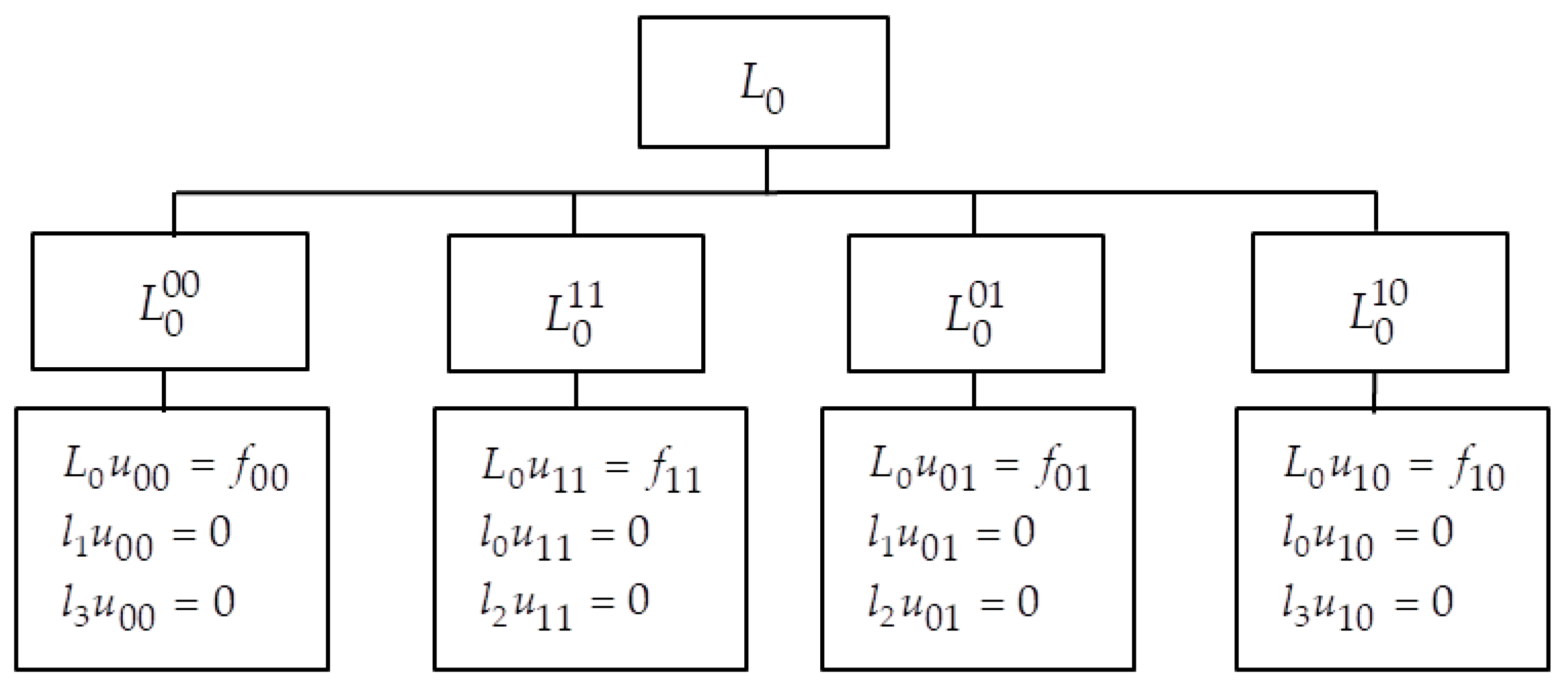
α = 0, we obtain a boundary value problem for an elliptic equation. This problem can be divided into two semi-homogeneous problems, (11), (12) and (13), (14), each of which is well researched, and it is a well-known fact that each of which has a single solution and holds inequality
L 1 u ( x , y ) L 0 u ( x , y ) = f ( x , y ) ,   α R , f L 2 ( K )
m = 1, 2
{ l m u u ( x , y ) | x = 0 + ( 1 ) m + 1 u ( x , y ) | x = 1 = 0 , l m + 2 u u ( x , y ) | y = 0 + ( 1 ) m + 1 u ( x , y ) | y = 1 = 0 ,
and
a f L 2 ( K ) 2 w W 2 2 ( K ) 2 b f L 2 ( K ) 2 ,   a , b > 0
Given that L 0 : H s j H s j ,   s , j = 0 , 1 , and operator L 0 has the representation L 0 = L 0 00   L 0 01   L 0 10 L 0 11 (which is easy to show), where   L 0 s j u = L 0 u ,   u H s j D ( L 0 ) ,   s , j = 0 , 1 .
We construct boundary value problems for each operator. The boundary value problems for each operator are shown in Figure 1.
L 1 u ( x , y ) L 0 u ( x , y ) = 0 ,   α R , f L 2 ( K )
m = 1, 2
{ l m u u ( x , y ) | x = 0 + ( 1 ) m + 1 u ( x , y ) | x = 1 = φ m ( y ) , l m + 2 u u ( x , y ) | y = 0 + ( 1 ) m + 1 u ( x , y ) | y = 1 = φ m + 2 ( x ) ,
u ( x , y ) W 2 2 ( K ) 2 C 1 j = 1 2 φ j W 2 3 2 ( 0 , 1 ) 2 + C 2 j = 3 4 φ j W 2 3 2 ( 0 , 1 ) 2 , C 1 , C 2 = c o n s t
Definition 1. 
The function u W 2 2 ( K ) is called a solution to problems (7)–(9) if the function u satisfies the conditions: L 1 u f L 2 ( K ) = 0 , l j u φ j W 2 3 2 ( 0 , 1 ) = 0 ,   j = 1 , 2 , 3 , 4 .
At first, we consider the problem (15), (16):
L 1 u ( x , y ) L 0 u ( x , y ) + α L 1 , x u ( x , y ) = f ( x , y ) ,   α R , f L 2 ( K )
u ( x , y ) | Γ = 0
Let L 1 be the task (15), (16) operator, L 1 u ( x , y ) L 1 u ( x , y ) ,   D ( L 1 ) = { u W 2 2 ( K ) , u | Γ = 0 } , and operator L 1 , x u ( x , y ) L 1 , x u ( x , y ) , D ( L 1 , x ) = D ( L 1 ) . Operator L 1 is the perturbation of operator L o .
When α = 0 , we get L 1 = L o for operators L 1 , L o , D ( L o ) = D ( L 1 ) .
Lemma 1. 
The operator L 1 , x has the following properties:
L 1 , x : H 0 j W 2 1 ( K ) 0 , L 1 , x : H 1 j W 2 1 ( K ) H 0 j , j = 0 , 1
.
Proof of Lemma 1. 
Since the operator has the form L 1 , x u ( x , y ) = D x u ( x , y ) D x u ( 1 x , y ) , and from the definition of the projector p 1 x and properties (1) and (2), we obtain
L 1 , x u ( x , y ) = D x ( u ( x , y ) u ( 1 x , y ) ) = 2 D x p 1 x u ( x , y )
Let u = p 0 x u H 0 j W 2 1 ( K ) , j = 0 , 1 , then L 1 , x : H 0 j W 2 1 ( K ) 0 , j = 0 , 1 .
Let u = p 1 x u H 1 j W 2 1 ( K ) ,   j = 0 , 1 , then using Formula (17) and the properties of operators (3)–(5), we obtain   L 1 , x u = 2 D x p 1 x p 1 x u = 2 D x p 1 x u = 2 p 0 x D x u H 0 j , j = 0 , 1 .
Finally, we get L 1 , x : H 1 j W 2 1 ( K ) H 0 j , j = 0 , 1 and L 1 , x : H 0 j W 2 1 ( K ) 0 , j = 0 , 1 . Lemma is proved. □
We consider the spectral problem:
Theorem 1. 
 
1. The pointwise spectrum of operator L 1 coincides with that of operator L 0 : σ p ( L 1 ) = σ p ( L 0 ) = { λ k , m : λ k , m = ( π k ) 2 + ( π m ) 2 ,   k , m N } .
2. System V ( L 1 ) of eigenvectors is complete and the minimal spanning system (set) of a space L 2 ( K ) .
Proof of Theorem 1. 
Operator L 0 has the eigenvalue { λ k , m : λ k , m = ( π k ) 2 + ( π m ) 2 ,   k , m N } and the system of eigenvectors V ( L 0 ) = { v k , m 0 L 2 ( K ) : v k , m 0 ( x , y ) = 2 sin ( π k x ) sin ( π m y ) ,   k , m N } .
Define eigenvectors of operator L 1 :
v k , m ( x , y ) = v k , m 0 ( x , y ) + v k , m 1 ( x , y ) , k , m N
where v k , m 0 ( x , y ) are eigenvectors of operator L 0 , k , m N .
If k = 2 s 1 then v 2 s 1 , m 0 H 0 j ,   j = 0 , 1 , L 1 , x v 2 s 1 , m 0 ( x , y ) = 0 follows from Lemma 1, and it also holds that L 1 v 2 s 1 , m 0 ( x , y ) = L 0 v 2 s 1 , m 0 ( x , y ) + α L 1 , x v 2 s 1 , m 0 ( x , y ) = L 0 v 2 s 1 , m 0 ( x , y ) .
Therefore, eigenvectors v 2 s 1 , m 0 ( x , y ) of operator L 0 are also eigenvectors of operator L 1 :
v 2 s 1 , m ( x , y ) = v 2 s 1 , m 0 ( x , y ) , s , m N
If k = 2 s , eigenvectors of operator L 1 are defined as below:
v 2 s , m ( x , y ) = v 2 s , m 0 ( x , y ) + v 2 s , m 1 ( x , y ) , s , m N
Let v 2 s , m 1 H 0 j , j = 0 , 1 , s , m N in the form of a series v 2 s , m 1 = r = 1 A s , m r sin ( 2 r 1 ) π x sin m π y , where A s , m r are unknown coefficients.
To determine the coefficients A k , m r , combining expression (20) and expression
L 1 v 2 s , m = λ 2 s , m v 2 s , m , we obtain
( L 0 λ 2 s , m ) v 2 s , m 1 ( x , y ) = α L 1 , x v 2 s , m 0 ( x , y ) ,
r = 1 A s , m r π 2 [ ( ( 2 r 1 ) 2 m 2 ) ( 2 s ) 2 m 2 ] sin ( 2 r 1 ) π x sin m π y = 8 α π s cos 2 s π x sin m π y .
On the other hand, cos 2 s π x = l = 1 4 ( 2 l 1 ) π ( ( 2 l 1 ) 2 ( 2 s ) 2 ) sin ( 2 l 1 ) π x . From the previous equality and the fact that the system { 2 sin π m y } m N is orthonormal of a Hilbert space L 2 ( 0 , 1 ) , we obtain
A s , m r = 32 α s ( 2 r 1 ) π 2 ( ( 2 r 1 ) 2 ( 2 s ) 2 ) 2 .
Finally, we have system V ( L 1 ) of eigenvectors:
{ v 2 s 1 , m ( x , y ) = 2 sin ( 2 s 1 ) π x sin m π y , s , m N ; v 2 s , m ( x , y ) = 2 sin 2 s π x sin m π y + r = 1 32 α s ( 2 r 1 ) π 2 ( ( 2 r 1 ) 2 ( 2 s ) 2 ) 2 sin ( 2 r 1 ) π x sin m π y .
Now, we want to prove that system V ( L 1 ) is complete.
We will prove it by this contradiction. For every h L 2 ( K ) using the properties of operators (6) h = h 1 , 1 + h 0 , 0 + h 0 , 1 + h 1 , 0 , where h i , j H i j ,   i , j = 0 , 1 . Let ( h , v k , m ) L 2 ( K ) = 0 , k , m N , v k , m V ( L 1 ) .
Let k = 2 s 1 , using Formulas (6) and (19), we obtain: ( h , v 2 s 1 , m ) L 2 ( K ) = ( h 1 , 1 + h 0 , 0 + h 0 , 1 + h 1 , 0 , v 2 s 1 , m 0 ) L 2 ( K ) = ( h 0 , 0 + h 0 , 1 , v 2 s 1 , m 0 ) L 2 ( K ) = 0 , s , m N .
If m = 2 l then ( h 0 , 0 + h 0 , 1 , v 2 s 1 , 2 l 0 ) L 2 ( K ) = ( h 0 , 1 , v 2 s 1 , 2 l 0 ) L 2 ( K ) = 0 , and using the fact that the system { v 2 s 1 , 2 l 0 } s , l = 1 is orthonormal of a space H 01 , we obtain h 0 , 1 ( x , y ) = 0 .
If m = 2 l 1 then ( h 0 , 0 , v 2 s 1 , 2 l 1 0 ) L 2 ( K ) = 0 ,   s , l N , and using the fact that the system { v 2 s 1 , 2 l 1 0 } s , l = 1 is orthonormal of a space H 00 , we obtain h 0 , 0 = 0 .
Let k = 2 s , using Formula (20) and inclusion v 2 s , m 1 H 0 j ,   j = 0 , 1 , we obtain ( h , v 2 s , m ) L 2 ( K ) = ( h 1 , 0 + h 1 , 1 , v 2 s , m ) L 2 ( K ) = ( h 1 , 0 + h 1 , 1 , v 2 s , m 0 + v 2 s , m 1 ) L 2 ( K ) = ( h 1 , 0 + h 1 , 1 , v 2 s , m 0 ) L 2 ( K ) , s , m N .
If m = 2 l 1 then ( h 1 , 0 + h 1 , 1 , v 2 s , 2 l 1 0 ) L 2 ( K ) = ( h 1 , 0 , v 2 s , 2 l 1 0 ) L 2 ( K ) = 0 ,   s , l N , and also using the fact that the system { v 2 s , 2 l 1 0 } s , l = 1 is orthonormal of a space H 01 , we obtain h 1 , 0 = 0 .
If m = 2 l then ( h 1 , 0 + h 1 , 1 , v 2 s , 2 l 0 ) L 2 ( K ) = ( h 1 , 1 , v 2 s , 2 l 0 ) L 2 ( K ) = 0 , s , l N ; similarly, one gets h 1 , 1 = 0 .
We conclude that h ( x , y ) 0 , which is a contradiction. We proved that system V ( L 1 ) is complete in the space of L 2 ( K ) .
Now, we want to prove that system V ( L 1 ) is the minimal spanning system (set) of a space L 2 ( K ) .
Define operator Q 1 as below:
{ Q 1 v 2 s 1 , m 0 ( x , y ) v 2 s 1 , m 0 ( x , y ) , s , m N Q 1 v 2 s , m 0 ( x , y ) v 2 s , m 0 ( x , y ) + v 2 s , m 1 ( x , y ) .
Let R 1 : L 2 ( K ) L 2 ( K ) , R 1 Q 1 E , and E : L 2 ( K ) L 2 ( K ) —identity operator L 2 ( K ) .
Therefore, using Formula (21), it holds that
{ R 1 v 2 s 1 , m 0 ( x , y ) 0 , s , m N R 1 v 2 s , m 0 ( x , y ) v 2 s , m 1 ( x , y ) .
Then, R 1 : H 1 j H 0 j , R 1 : H 0 j 0 , j = 0 , 1 . Operator R 1 is the transformation operator and it follows that operators Q 1 1 and ( Q 1 ) 1 exist:
Q 1 1 = E R 1 , ( Q 1 ) 1 = ( E + R 1 * ) 1 = E R 1 *
Using Formula (22), define the elements of the system W ( L 1 ) biorthogonal to the system V ( L 1 ) : w ( x , y ) = ( Q 1 1 ) * v ( x , y ) , where v V ( L 1 ) . System V ( L 1 ) of eigenvectors is the minimal spanning system (set) of a space L 2 ( K ) . Theorem 1 is proved. □
Theorem 2. 
The system of eigenvectors V ( L 1 ) is a Riesz basis of a space L 2 ( K ) .
Proof of Theorem 2. 
We will prove that operator R 1 is bounded.
For every h L 2 ( K ) , we have h = k , m = 1 h k , m v k , m 0 ( x , y ) .
R 1 h L 2 ( K ) 2 = R 1 k , m = 1 h k , m v k , m 0 L 2 ( K ) 2 = s , m = 1 h 2 s , m R 1 v 2 s , m 0 L 2 ( K ) 2 = s , m = 1 h 2 s , m v 2 s , m 1 L 2 ( K ) 2 .
Using equality: ( 2 x 1 ) sin 2 k π x = r = 1 32 k ( 2 r 1 ) π 2 ( ( 2 r 1 ) 2 ( 2 k ) 2 ) 2 sin ( 2 r 1 ) π x .
We obtain R 1 h L 2 ( K ) 2 = s , m = 1 h 2 s , m α ( 2 x 1 ) sin 2 s π x sin m π y L 2 ( K ) 2 C 3 s , m = 1 | h 2 s , m | 2 C 4 h L 2 ( K ) 2 , C 3 , C 4 = c o n s t , where C 4 = α 2 12 .
Operators Q 1 1 = E R 1 , Q 1 = E + R 1 are bounded to a space L 2 ( K ) . Following the theorem [22], we obtain that the system of eigenvectors V ( L 1 ) is a Riesz basis of a space L 2 ( K ) .
Theorem 2 is proved. □
We consider a boundary value problem:
L 1 w ( x , y ) = L 0 w ( x , y ) + α L 1 , x w ( x , y ) = f ( x , y ) ,   α R , f L 2 ( K ) ,
L 0 w ( x , y ) = Δ w ( x , y ) = ( D x 2 w ( x , y ) + D y 2 w ( x , y ) ) ,
L 1 , x w ( x , y ) = D x w ( x , y ) D x w ( 1 x , y ) .
w ( x , y ) | x = 0 + w ( x , y ) | x = 1 = φ 1 ( y ) , w ( x , y ) | x = 0 w ( x , y ) | x = 1 = φ 2 ( y ) , w ( x , y ) | y = 0 + w ( x , y ) | y = 1 = φ 3 ( x ) , w ( x , y ) | y = 0 w ( x , y ) | y = 1 = φ 4 ( x ) ,
where φ s W 2 3 2 ( 0 , 1 ) ,   s = 1 , 2 , 3 , 4 .
Now, let us proceed to problem (23), (24).
The function w ( x , y ) can be presented as the sum w ( x , y ) = u ( x , y ) + z ( x , y ) . Functions u ( x , y ) , z ( x , y ) are solutions to the following problems:
L 1 u ( x , y ) = L 0 u ( x , y ) + α L 1 , x u ( x , y ) = f ( x , y ) ,   α R , f L 2 ( K ) { u ( x , y ) | x = 0 + u ( x , y ) | x = 1 = 0 , u ( x , y ) | x = 0 u ( x , y ) | x = 1 = 0 , u ( x , y ) | y = 0 + u ( x , y ) | y = 1 = 0 , u ( x , y ) | y = 0 u ( x , y ) | y = 1 = 0 ,
L 1 z ( x , y ) = L 0 z ( x , y ) + α L 1 , x z ( x , y ) = 0 ,   α R , { z ( x , y ) | x = 0 + z ( x , y ) | x = 1 = φ 1 ( y ) , z ( x , y ) | x = 0 z ( x , y ) | x = 1 = φ 2 ( y ) , z ( x , y ) | y = 0 + z ( x , y ) | y = 1 = φ 3 ( x ) , z ( x , y ) | y = 0 z ( x , y ) | y = 1 = φ 4 ( x ) .
Theorem 3. 
If f L 2 ( K ) then a unique solution to problem (25) exists and satisfies the following estimate:
u L 2 ( K ) 2 C f L 2 ( K ) 2 .
Proof of Theorem 3. 
Now let us proceed to problem (25). The function u ( x , y ) , f ( x , y ) can be presented as a sum:
u ( x , y ) = u   1 , 0 ( x , y ) + u 1 , 1 ( x , y ) + u 0 , 0 ( x , y ) + u 0 , 1 ( x , y ) , f ( x , y ) = f 1 , 0 ( x , y ) + f 1 , 1 ( x , y ) + f 0 , 0 ( x , y ) + f 0 , 1 ( x , y ) ,
where u s , j H s j W 2 2 ( K ) , f s , j H s j ,   s , j = 0 , 1 .
Combining both expressions (25) and (28), we obtain
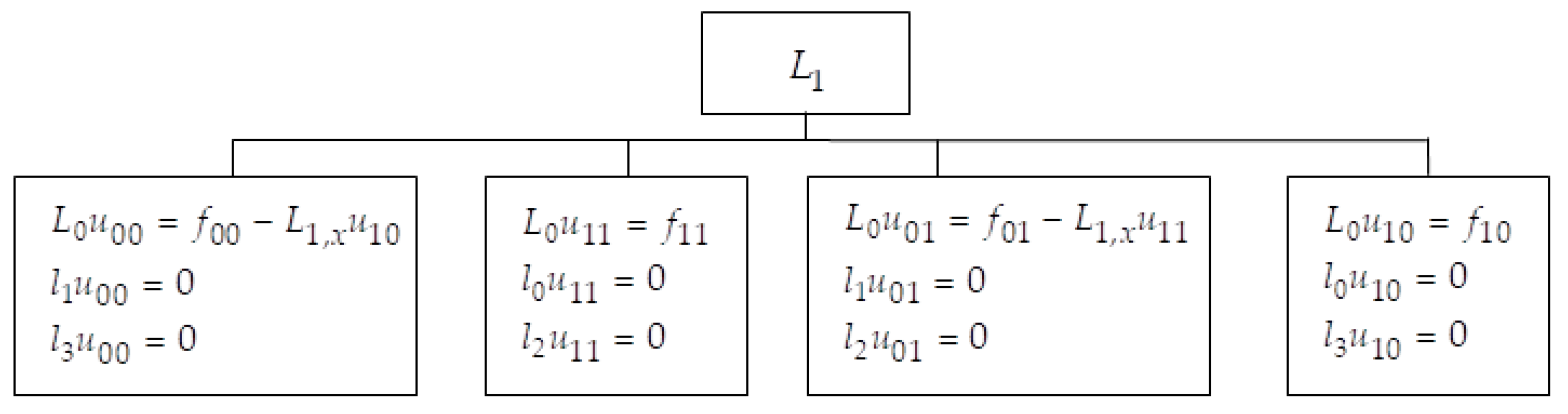
( L 0 + L 1 , x ) s , j = 0 1 u s , j = s , j = 0 1 f s , j ,
s , j = 0 1 L 0 u s , j + s , j = 0 1 L 1 , x u s , j = s , j = 0 1 f s , j ,
{ s , j = 0 1 u s , j ( x , y ) | x = 0 + s , j = 0 1 u s , j ( x , y ) | x = 1 = 0 , s , j = 0 1 u s , j ( x , y ) | x = 0 s , j = 0 1 u s , j ( x , y ) | x = 1 = 0 , s , j = 0 1 u s , j ( x , y ) | y = 0 + s , j = 0 1 u s , j ( x , y ) | y = 1 = 0 , s , j = 0 1 u s , j ( x , y ) | y = 0 s , j = 0 1 u s , j ( x , y ) | y = 1 = 0 .
Using Lemma 1 (Figure 2), it also holds that L 1 , x u 0 , j ( x , y ) = 0 ,   j = 0 , 1 and
s , j = 0 1 L 0 u s , j + L 1 , x u 1 , 0 + L 1 , x u 1 , 1 = s , j = 0 1 f s , j
We solve each of these problems similarly to problems (11) and (12).
Using the properties of operator (4) and inclusion L 1 , x u 1 , 0 H 00 , L 1 , x u 1 , 1 H 01 (following Lemma 1), problem (25) is divided into parts:
L 0 u 1 , 0 ( x , y ) = f 1 , 0 ( x , y ) , { u 1 , 0 ( x , y ) | x = 0 + u 1 , 0 ( x , y ) | x = 1 = 0 , u 1 , 0 ( x , y ) | x = 0 u 1 , 0 ( x , y ) | x = 1 = 0 , u 1 , 0 ( x , y ) | y = 0 + u 1 , 0 ( x , y ) | y = 1 = 0 , u 1 , 0 ( x , y ) | y = 0 u 1 , 0 ( x , y ) | y = 1 = 0 ,
L 0 u 1 , 1 ( x , y ) = f 1 , 1 ( x , y ) , { u 1 , 1 ( x , y ) | x = 0 + u 1 , 1 ( x , y ) | x = 1 = 0 , u 1 , 1 ( x , y ) | x = 0 u 1 , 1 ( x , y ) | x = 1 = 0 , u 1 , 1 ( x , y ) | y = 0 + u 1 , 1 ( x , y ) | y = 1 = 0 , u 1 , 1 ( x , y ) | y = 0 u 1 , 1 ( x , y ) | y = 1 = 0 ,
L 0 u 00 ( x , y ) = f 00 ( x , y ) L 1 , x u 10 ( x , y ) , { u 0 , 0 ( x , y ) | x = 0 + u 0 , 0 ( x , y ) | x = 1 = 0 , u 0 , 0 ( x , y ) | x = 0 u 0 , 0 ( x , y ) | x = 1 = 0 , u 0 , 0 ( x , y ) | y = 0 + u 0 , 0 ( x , y ) | y = 1 = 0 , u 0 , 0 ( x , y ) | y = 0 u 0 , 0 ( x , y ) | y = 1 = 0 ,
L 0 u 0 , 1 ( x , y ) = f 0 , 1 ( x , y ) L 1 , x u 1 , 1 ( x , y ) , { u 0 , 1 ( x , y ) | x = 0 + u 0 , 1 ( x , y ) | x = 1 = 0 , u 0 , 1 ( x , y ) | x = 0 u 0 , 1 ( x , y ) | x = 1 = 0 , u 0 , 1 ( x , y ) | y = 0 + u 0 , 1 ( x , y ) | y = 1 = 0 , u 0 , 1 ( x , y ) | y = 0 u 0 , 1 ( x , y ) | y = 1 = 0 .
Problems (29) and (30) are similar to problems (11) and (12). There are unique solutions to each of the problems (29) and (30) and they hold inequality
M i f 1 , i L 2 ( K ) 2 u 1 , i W 2 2 ( K ) 2 L i f 1 , i L 2 ( K ) 2 , M i , L i > 0 , i = 0 , 1 .
For problems (31) and (32), we prove that f 0 , 0 L 1 , x u 1 , 0 L 2 ( K ) and f 0 , 1 L 1 , x u 1 , 1 L 2 ( K ) :
f 0 , 0 L 1 , x u 1 , 0 L 2 ( K ) 2 2 ( f 0 , 0 L 2 ( K ) 2 + L 1 , x u 1 , 0 L 2 ( K ) 2 )
2 ( f 0 , 0 L 2 ( K ) 2 + 4 D x u 1 , 0 L 2 ( K ) 2 ) 2 ( f 0 , 0 L 2 ( K ) 2 + 4 | α | 2 D α u 1 , 0 L 2 ( K ) 2 )
2 ( f 0 , 0 L 2 ( K ) 2 + 4 C 5 u 1 , 0 W 2 2 ( K ) 2 ) < ,
f 0 , 1 L 1 , x u 1 , 1 L 2 ( K ) 2 2 ( f 0 , 1 L 2 ( K ) 2 + L 1 , x u 1 , 1 L 2 ( K ) 2 ) 2 ( f 0 , 1 L 2 ( K ) 2 + 4 C 6 u 1 , 1 W 2 2 ( K ) 2 ) < .
We proved that problems (29) and (30) are similar to problems (11) and (12). So, there is a unique solution to these problems and it holds inequality
C ¯ i f 0 , i L 2 ( K ) 2 u 0 , i W 2 2 ( K ) 2 C i f 0 , i L 2 ( K ) 2 , i = 0 , 1 , C ¯ i , C i > 0
Following the previous results and equality: u L 2 ( K ) 2 = u 0 , 1 L 2 ( K ) 2 + u 1 , 0 L 2 ( K ) 2 + u 1 , 1 L 2 ( K ) 2 + u 0 , 0 L 2 ( K ) 2 , we obtain the existence of a unique solution to problem (25) that satisfies inequality (27).
Theorem 3 is proved. □
Solution z ( x , y ) of problem (25) can be presented as a sum:
z ( x , y ) = v 1 ( x , y ) + v 2 ( x , y ) , where v 1 ( x , y ) , v 2 ( x , y ) are the solutions to problems (33) and (34):
L 1 v 1 ( x , y ) = L 0 v 1 ( x , y ) + α L 1 , x v 1 ( x , y ) = 0 , { v 1 ( x , y ) | x = 0 + v 1 ( x , y ) | x = 1 = φ 1 ( y ) , v 1 ( x , y ) | x = 0 v 1 ( x , y ) | x = 1 = φ 2 ( y ) , v 1 ( x , y ) | y = 0 + v 1 ( x , y ) | y = 1 = 0 , v 1 ( x , y ) | y = 0 v 1 ( x , y ) | y = 1 = 0 .
L 1 v 2 ( x , y ) = L 0 v 2 ( x , y ) + α L 1 , x v 2 ( x , y ) = 0 , { v 2 ( x , y ) | x = 0 + v 2 ( x , y ) | x = 1 = 0 , v 2 ( x , y ) | x = 0 v 2 ( x , y ) | x = 1 = 0 , v 2 ( x , y ) | y = 0 + v 2 ( x , y ) | y = 1 = φ 3 ( x ) , v 2 ( x , y ) | y = 0 v 2 ( x , y ) | y = 1 = φ 4 ( x ) .
We rewrite problem (33) in differential-operator form, and it is defined as operator B 2 : L 2 ( 0 , 1 ) L 2 ( 0 , 1 ) ,   B 2 h ( y ) d 2 h ( y ) d y 2 , D ( B 2 ) = { h W 2 2 ( 0 , 1 ) : h ( 0 ) = h ( 1 ) = 0 } .
Since operator B 2 is positively defined, then operator A 2 exists:
A 2 B 2 ,   D ( A 2 ) = { h = k h k 2 sin k π y L 2 ( 0 , 1 ) : k k 2 | h k | 2 < }
Let H = L 2 ( 0 , 1 ) ,   v 1 ( x , y ) = v 1 ( x ) , φ 1 = φ 1 ( y ) H , φ 2 = φ 2 ( y ) H ,
α L 1 , x v 1 ( x , y ) α L 1 , x v 1 ( x ) = α D x ( v 1 ( x ) v 1 ( 1 x ) ) .
Problem (33) has a differential-operator formulation:
{ D x 2 v 1 ( x ) + A 2 2 v 1 ( x ) + α L 1 , x 1 v 1 ( x ) = 0 , v 1 ( x ) | x = 0 + v 1 ( x ) | x = 1 = φ 1 , v 1 ( x ) | x = 0 v 1 ( x ) | x = 1 = φ 2 .
Further, we rewrite problem (34) in differential-operator form.
Define operator: B 1 : L 2 ( 0 , 1 ) L 2 ( 0 , 1 ) , B 1 g ( x ) d 2 g ( x ) d x 2 + α L x 1 g ( x ) , α R ,
D ( B 1 ) = { g W 2 2 ( 0 , 1 ) : g ( 0 ) = g ( 1 ) = 0 } .
Since operator B 1 is positively defined, there is the operator
A 1 B 1 , D ( A 1 ) = { g ( x ) = k g k 2 sin k π x L 2 ( 0 , 1 ) : k k 2 | g k | 2 < } .
Let H = L 2 ( 0 , 1 ) , v 2 ( y ) = v 2 ( x , y ) , φ 3 = φ 3 ( x ) H , φ 4 = φ 4 ( x ) H .
Problem (34) has a differential-operator formulation:
{ D y 2 v 2 ( y ) + A 1 2 v 2 ( y ) = 0 , v 2 ( y ) | y = 0 + v 2 ( y ) | y = 1 = φ 3 , v 2 ( y ) | y = 0 v 2 ( y ) | y = 1 = φ 4 .
Problems (35) and (36) were researched [25], each of which has a single solution and holds inequalities
v 1 W 2 2 ( K ) 2 C 6 ( φ 2 W 2 3 2 ( 0 , 1 ) 2 + φ 1 W 2 3 2 ( 0 , 1 ) 2 )   and   v 2 W 2 2 ( ( 0 , 1 ) ; H ) 2 C 7 ( φ 0 H ( A 3 2 ) 2 + φ 1 H ( A 3 2 ) 2 ) .
Additionally, they hold
z W 2 2 ( K ) 2 C 8 ( v 1 W 2 2 ( K ) 2 + v 2 W 2 2 ( K ) 2 ) ,
where C 8 = max { 2 C 6 , 2 C 7 } .
Theorem 4. 
For every f L 2 ( K ) and φ 1 , φ 2 ,   φ 3 , φ 4 W 2 3 2 ( 0 , 1 ) exists a unique solution, w ( x , y ) W 2 2 ( K ) , to problems (25) and (26) which satisfies the following inequality:
w W 2 2 ( K ) 2 C 9 ( f L 2 ( K ) 2 + j = 1 2 φ j W 2 3 2 ( 0 , 1 ) 2 + j = 3 4 φ j W 2 3 2 ( 0 , 1 ) 2 ) .
Proof of Theorem 4. 
The existence of a single solution, w = u + z , to problems (22) and (24) follows from the existence of solutions to problems (25) and (26), respectively, of Theorem 3, and for Formula (38), a unique solution, w , exists and holds inequality w L 2 ( K ) 2 2 ( u L 2 ( K ) 2 + z L 2 ( K ) 2 ) , therefore, by adding inequalities (27) and (38), we obtain inequality (39), where C 9 = max { 2 C , 2 C 8 } .
Theorem 4 is proved. □

4. Conclusions

We investigated the Dirichlet problem for the elliptic equation perturbed by the selected variable and established the spectral properties of the perturbed operator. Further, we explicitly found the eigenvalues and eigenfunctions of the perturbed task operator. We proved the isospectrality of the perturbed operator to the operator of the Dirichlet problem for an elliptic equation and proved the completeness, minimality, and basicity of the system of eigenfunctions of this operator. We proved the theorem on the existence and uniqueness of the solution to the boundary value problem for a perturbed elliptic equation. We obtained an upper bound solution to the researched problem.
Similar results we can obtain if we consider the perturbations are of the following forms:
L 2 , x u ( x , y ) = D x u ( x , y ) + D x u ( 1 x , y )
L 1 , y u ( x , y ) = D y u ( x , y ) D y u ( x , 1 y ) ,
L 2 , y u ( x , y ) = D y u ( x , y ) + D y u ( x , 1 y ) ,
L 2 , x u ( x , y ) = D x u ( x , y ) + D x u ( 1 x , y ) ,
L 1 , y u ( x , y ) = D y u ( x , y ) D y u ( x , 1 y ) ,
L 2 , y u ( x , y ) = D y u ( x , y ) + D y u ( x , 1 y ) ,
L 1 , x y u ( x , y ) = D x ( u ( x , y ) u ( 1 x , 1 y ) )
In further research, we plan to show the general class of perturbations for elliptic equations of the Dirichlet problem and the study of the Dirichlet problem for differential equations in partial derivatives of higher orders. We will also show the selection of isospectrality classes for such a problem and proof of the theorems of existence and uniqueness of the solution to such problems.

Author Contributions

Studies analysis, U.Y.; methodology, U.Y. and S.F.; resources, S.F. and U.Y.; validation, U.Y.; writing—original draft preparation, U.Y. and S.F.; writing—review and editing, U.Y., S.F. and P.V.; visualization, U.Y., and S.F.; project administration, S.F. All authors have read and agreed to the published version of the manuscript.

Funding

This research received no external funding.

Conflicts of Interest

The authors declare no conflict of interest.

References

  1. Azbelev, N.; Maksimov, V.; Simonov, P. Functional-differential equations and their applications. Vestn. Udmurt. Univ. Mat. Fur. Comput. Sci. 2009, 1, 3–23. [Google Scholar] [CrossRef] [Green Version]
  2. Bitsadze, A. Some Classes of Partial Differential Equations; CRC Press: Boca Raton, FL, USA, 1988; p. 504. [Google Scholar]
  3. Gorbachuk, V.; Gorbachuk, M. Some questions of the spectral theory of differential equations in the space of vector functions on a finite interval. Ukr. Mat. J. 1976, 28, 12–26. [Google Scholar] [CrossRef]
  4. Gorbachuk, V.; Gorbachuk, M. Boundary Value Problems for Differential Operator Equations; Springer: Berlin/Heidelberg, Germany, 1984; 284p. [Google Scholar]
  5. Myshkis, A. Mixed functional differential equations. In Contemporary Mathematics. Fundamental Directions; Peoples’ Friendship University of Russia: Moscow, Russia, 2003; Volume 4, pp. 5–120. [Google Scholar]
  6. Rossovskii, L.E.; Skubachevsky, A.L. Solvability and regularity of solutions for some classes of elliptic functional-differential equations. J. Math. Sci. 2001, 104, 1008–1011. [Google Scholar] [CrossRef]
  7. Skubachevsky, A. On the spectrum of some nonlocal elliptic boundary value problems. Mat. Sat. 1982, 117, 548–558. [Google Scholar] [CrossRef]
  8. Yakubov, S. Linear Differential-Operator Equations and Their Transformations; ELM: Baku, Azerbaijan, 1985; 189p. [Google Scholar]
  9. Yakubov, S.; Mamedov, K. Completeness of eigenfunctions and associated functions of some irregular boundary value problems for ordinary differential equations. Funk. Anal. Appl. 1980, 14, 93–94. [Google Scholar]
  10. Phage, M.; Nagnibida, N. The Equivalence Problem for Ordinary Linear Differential Operators. Available online: https://iopscience.iop.org/article/10.1088/1742-6596/621/1/012002/pdf (accessed on 12 September 2020).
  11. Izonin, I.; Kryvinska, N.; Vitynskyi, P.; Tkachenko, R.; Zub, K. Grnn approach towards missing data recovery between iot systems. Adv. Intell. Syst. Comput. 2020, 1035, 445–453. [Google Scholar]
  12. Dronyuk, I.; Verhun, V.; Kryvinska, N. The mathematical model for ranking students of online IT courses. CEUR Workshop Proc. 2019, 2533, 107–116. [Google Scholar]
  13. Hoshovska, O.; Poplavska, Z.; Kryvinska, N.; Horbal, N. Considering random factors in modeling complex microeconomic systems. Mathematics 2020, 8, 1206. [Google Scholar] [CrossRef]
  14. Fedushko, S.; Ustyianovych, T.; Gregus, M. Real-time high-load infrastructure transaction status output prediction using operational intelligence and big data technologies. Electronics 2020, 9, 668. [Google Scholar] [CrossRef] [Green Version]
  15. Kryvinska, N. An analytical approach for the modeling of real-time services over IP network. Math. Comput. Simul. 2008, 79, 980–990. [Google Scholar] [CrossRef]
  16. Baskakov, A. Harmonic Analysis of Linear Operators; Voronezh State University: Voronezh, Russia, 1987; 164p. [Google Scholar]
  17. Aibeche, A. Coerciveness inequality for nonlocal boundary value problems for second order abstract elliptic differential equations. J. Inequ. Appl. Math. 2003, 4, 80–109. [Google Scholar]
  18. Aibeche, A.; Amroune, N.; Maingot, S. On elliptic equations with general non-local boundary conditions in UMD spaces. Mediterr. J. Math. 2016, 13, 1051–1063. [Google Scholar] [CrossRef]
  19. Kritskov, L.V.; Sarsenbi, A.M. Spectral properties of a nonlocal problem for a second-order differential equation with an involution. Differ. Equ. 2015, 51, 984–990. [Google Scholar] [CrossRef]
  20. Ashyralyev, A.; Sarsenbi, A.M. Well-posedness of an elliptic equations with an involution. Electr. J. Differ. Equ. 2015, 284, 1–8. [Google Scholar]
  21. Cabada, A.; Tojo, F. Existence results for a linear equation with reflection, non-constant coefficient and periodic boundary conditions. J. Math. Anal. Appl. 2014, 412, 529–546. [Google Scholar] [CrossRef]
  22. Kirane, M.; Al-Salti, N. Inverse problems for a nonlocal wave equation with an involution perturbation. J. Nonlinear Sci. Appl. 2016, 9, 1243–1251. [Google Scholar] [CrossRef]
  23. Kalenyuk, P.; Baranetsky, Y.; Nitrebich, Z. Generalized Method of Separating Variables; Naukova Dumka: Kyiv, Ukraine, 1993; 232p. [Google Scholar]
  24. Baranetsky, Y.; Yarka, U. On a class of boundary value problems for integro-differential equations. Bull. LPNU Appl. Math. 1999, 364, 310–315. [Google Scholar]
  25. Baranetsky, Y.; Yarka, U. On a class of boundary value problems for differential equations of even order–Operator. Matt. Methods Phys. Fur. Polya. 1999, 2, 1–6. [Google Scholar]
  26. Baranetskij, Y.; Yarka, U. Solution of boundary value problems for abstract differential equations. In International Conference on Functional Analysis and Its Applications; Lviv Ivan Franko National University: Lviv, Ukraine, 2002; p. 29. [Google Scholar]
  27. Baranetskij, Y.; Yarka, U.B.; Fedushko, S. Abstract perturbations of the Dirichlet differential operator. Spectral properties. Sci. Bull. Uzhg. Univ. Ser. Mat. Inf. 2012, 3, 12–16. [Google Scholar]
  28. Baranetskij, Y.; Basha, A. Nonlocal multipoint problem for differential-operator equations of order 2n. J. Math. Sci. 2016, 217, 176–186. [Google Scholar] [CrossRef]
  29. Baranetskij, Y.; Kolyasa, L. Boundary-value problem for abstract second-order differential equation with involution. Bull. Lpnu Phys. Math. Sci. 2017, 871, 20–27. [Google Scholar]
  30. Baranetskij, Y.O.; Kalenyuk, P.I.; Kolyasa, L.I. Boundary-value problem for abstract differential equations with operator involution. Bukov. Math. J. 2016, 4, 22–29. [Google Scholar]
  31. Baranetsky, Y.O.; Kaleniuk, P.I.; Yarka, U.B. Perturbations boundary value problems for ordinary differential equations of the second order. Bull. LPNU Appl. Math. 1998, 337, 70–73. [Google Scholar]
  32. Tribel, H. Interpolation Theory. Functional Spaces, Differential Operators; Johann Ambrosius Barth Verlag: Heidelberg, Germany; Leipzig, Germany, 1987. [Google Scholar]
Figure 1. Boundary value problems for operators L 0 s j ,   i , j = 0 , 1 .
Mathematics 08 02108 g001
Figure 2. Division of a boundary value problem for a perturbed operator L 1 into parts according to subspaces H i j ,   i , j = 0 , 1 .
Mathematics 08 02108 g002
Publisher’s Note: MDPI stays neutral with regard to jurisdictional claims in published maps and institutional affiliations.

