Optimal Control Problem Solution with Phase Constraints for Group of Robots by Pontryagin Maximum Principle and Evolutionary Algorithm

Abstract

A numerical method based on the Pontryagin maximum principle for solving an optimal control problem with static and dynamic phase constraints for a group of objects is considered. Dynamic phase constraints are introduced to avoid collisions between objects. Phase constraints are included in the functional in the form of smooth penalty functions. Additional parameters for special control modes and the terminal time of the control process were introduced. The search for additional parameters and the initial conditions for the conjugate variables was performed by the modified self-organizing migrating algorithm. An example of using this approach to solve the optimal control problem for the oncoming movement of two mobile robots is given. Simulation and comparison with direct approach showed that the problem is multimodal, and it approves application of the evolutionary algorithm for its solution.

1. Introduction

The optimal control belongs to complex computational problems for which there are no universal solution algorithms. The most well-known result in this area [1] transforms the optimization problem into a boundary-value problem, and the dimension of the problem doubles. The goal of solving the boundary-value problem is to find the initial conditions for conjugate variables such that the vector of state variables falls into a given terminal condition. In general, for this problem, there is no guarantee that the functional for the boundary-value problem is not unimodal and convex on the space of initial conditions of conjugate variables.

The optimal control problem with phase constraints is considered. Phase constraints are included in the functional, so they are included in the system of equations for conjugate variables. This greatly complicates the analysis of the problem on the convexity and unimodality of the target functional. The accurate solution of optimal control problem has to use additional functions and regularization of equations at the search of control [2,3]. An additional problem in solving a boundary-value problem is determination of time for checking the fulfillment of boundary conditions.

In this paper, for the numerical solution of the problem, it is proposed to use evolutionary algorithms that have shown efficiency in solving optimal control problems [4]. SOMA is a universal algorithm for various difficult optimization problems [5,6]. However, our attempt to apply SOMA to the optimal control problem of four robots with constraints has failed to find a good solution for any values of the algorithm parameters. We supposed that the modification of each possible solution in population in the process of evolution using the best current possible solution is not enough [7]. We expanded the modification of SOMA by introducing the best historical solution among randomly selected ones for each possible solution in the population.

The article consists of an introduction and eight sections. Statement of the optimal control problem with phase constraints is presented in Section 2. Section 3 contains Pontryagin maximum principle as one of main approaches for its numerical solution. Section 4 contains a description of one of the evolutionary algorithms, modified SOMA. An example is given in Section 5. The computational experiment and results are presented in Section 6. Section 7 describes the search of optimal control by direct method. Alternative non-deterministic control methods are observed in Section 8. Results and future research directions are discussed in Section 9.

2. Optimal Control Problem with Phase Constraints for Group of Robots

Consider the problem of optimal control for a group of robots with phase constraints. Given a mathematical model of control objects in the form of the system of ordinary differential equations

$${\dot{\mathbf{x}}}^j={\mathbf{f}}^j({\mathbf{x}}^j,{\mathbf{u}}^j),$$

(1)

where ${\mathbf{x}}^j$ is a state space vector of control object j, ${\mathbf{x}}^j\in {\mathbb{R}}^{n_j}$, ${\mathbf{u}}^j$ is a control vector of object j, ${\mathbf{u}}^j\in {\mathrm{U}}^j\subseteq {\mathbb{R}}^{m_j}$, ${\mathrm{U}}^j$ is a compact limited set, $m_j⩽n_j$, $j=1,\dots ,M$, M is a number of objects. For the system (1) initial conditions are given

$${\mathbf{x}}^j\left(0\right)={\mathbf{x}}^{j,0}\in {\mathbb{R}}^{n_j},j=1,\dots ,M.$$

(2)

Given terminal conditions

$${\mathbf{x}}^j\left(t_{f,j}\right)={\mathbf{x}}^{j,f}\in {\mathbb{R}}^{n_j},$$

(3)

where $t_{f,j}$ is an unknown limited positive value, that corresponds to time when object j achieves its terminal position

$$t_{f,j}⩽t^{+},$$

(4)

$t^{+}$ is a given time of achievement of terminal conditions (3),

$$t_{f,j}=\left\{\begin{array}{c}t,ift<t^{+}and\parallel {\mathbf{x}}^j\left(t\right)-{\mathbf{x}}^{j,f}\parallel ⩽{\epsilon }_1\hfill \\ t^{+},\mathrm{otherwise}\hfill \end{array}\right.,$$

(5)

${\epsilon }_1$ is a small positive value, $j=1,\dots ,M$. The phase constraints are given

$${\phi }_i\left({\mathbf{x}}^j\left(t\right)\right)⩽0,i=1,\dots ,r,j=1,\dots ,M.$$

(6)

The conditions of collision avoidance are described as

$$\chi ({\mathbf{x}}^j\left(t\right),{\mathbf{x}}^k\left(t\right))⩽0,j=1,\dots ,M-1,k=j+1,\dots ,M.$$

(7)

The quality functional is given in general integral form

$$J_0=\underset{0}{\overset{t_f}{\int }}{f}_0({\mathbf{x}}^1\left(t\right),\dots ,{\mathbf{x}}^M\left(t\right),{\mathbf{u}}^1\left(t\right),\dots ,{\mathbf{u}}^M\left(t\right))dt\to min,$$

(8)

where

$$t_f=max\{t_{f,1},\dots ,t_{f,M}\}.$$

(9)

It is necessary to find control as a time function

$${\mathbf{u}}^j={\mathbf{v}}^j\left(t\right),j=1,\dots ,M,$$

(10)

in order to provide terminal conditions (3) with optimal value of functional (8) without violation of constraints (6) and with collision avoidance (7). For a numerical solution of the problem, let us insert phase constraints and terminal conditions in quality functional (8)

$$J_1=\underset{0}{\overset{t_f}{\int }}{f}_0({\mathbf{x}}^1\left(t\right),\dots ,{\mathbf{x}}^M\left(t\right),{\mathbf{u}}^1\left(t\right),\dots ,{\mathbf{u}}^M\left(t\right))dt+a\underset{0}{\overset{t_f}{\int }}\sum _{i=1}^r\sum _{j=1}^M{\mu }^2\left({\phi }_i\left({\mathbf{x}}^j\left(t\right)\right)\right)dt+$$

$$b\underset{0}{\overset{t_f}{\int }}\sum _{j=1}^{M-1}\sum _{k=j+1}^M{\mu }^2\left(\chi ({\mathbf{x}}^j\left(t\right),{\mathbf{x}}^k\left(t\right))\right)dt+c\sum _{j=1}^M\left|\right|{\mathbf{x}}^j\left(t_f\right)-{\mathbf{x}}^{j,f}\left|\right|\to min,$$

(11)

where a, b, c are given positive weight coefficients, $\mu \left(A\right)=max\{0,A\}$.

To solve the problem stated above, we use the Pontryagin maximum principle.

3. The Pontryagin Maximum Principle

The Pontryagin maximum principle allows one to transform the problem of optimization on infinite dimensional space to the boundary-value problem for the system of differential Equations (1). Let us construct Hamilton function for this problem on the base of the system (2) and the quality functional (2) without terminal conditions

$$H({\mathbf{x}}^1,\dots ,{\mathbf{x}}^M,{\mathbf{u}}^1,\dots ,{\mathbf{u}}^M,\psi )=-f_0({\mathbf{x}}^1,\dots ,{\mathbf{x}}^M,{\mathbf{u}}^1,\dots ,{\mathbf{u}}^M)-$$

$$a\sum _{i=1}^r\sum _{j=1}^M{\mu }^2\left({\phi }_i\left({\mathbf{x}}^j\right)\right)-b\sum _{j=1}^{M-1}\sum _{k=j+1}^M{\mu }^2\left(\chi ({\mathbf{x}}^j,{\mathbf{x}}^k)\right)+{\psi }^T{\mathbf{f}}^j({\mathbf{x}}^j,{\mathbf{u}}^j),$$

(12)

where $\psi ={[{\psi }_1\dots {\psi }_n]}^T$ is a vector of conjugate variables, $n=n_1+\dots +n_M$,

$$\dot{\psi }=-\frac{\partial H({\mathbf{x}}^1,\dots ,{\mathbf{x}}^M{\mathbf{u}}^1,\dots ,{\mathbf{u}}^M,\psi )}{\partial {\mathbf{x}}^1,\dots ,\partial {\mathbf{x}}^M}.$$

(13)

According to the Pontryagin maximum principle, a necessary condition for optimal control is the maximum of Hamilton function (12)

$$\underset{{\mathbf{u}}^1\in {\mathrm{U}}^1,\dots ,{\mathbf{u}}^M\in {\mathrm{U}}^M}{max}H({\mathbf{x}}^1,\dots ,{\mathbf{x}}^M,{\mathbf{u}}^1,\dots ,{\mathbf{u}}^M,\psi ).$$

(14)

Pontryagin maximum principle allows one to transform the optimal control problem to a boundary-value problem. It is necessary to find the initial values of conjugate variables so that the state vector reaches terminal conditions (3). To solve the boundary-value problem, we have to solve a finite dimensional problem of nonlinear programming with the following functional

$$F\left(\mathbf{q}\right)=\sum _{j=1}^M\parallel {\mathbf{x}}^j\left(t_{f,j}\right)-{\mathbf{x}}^{j,f}\parallel \to \underset{\mathbf{q}\in \mathrm{Q}}{min},$$

(15)

where $\mathbf{q}={[q_1\dots q_n]}^T$, $\mathrm{Q}$ is a limited compact set, $q_i={\psi }_i\left(0\right)$, $i=1,\dots ,n$,

$$\sum _{i=1}^n{q}_i^2=1.$$

(16)

In a boundary-value problem, it is not known exactly when it is necessary to check the boundary conditions (15). The maximum principle does not provide equations for definition of terminal time $t_{f,j}$ of the control process, while a numerical search of some possible solutions may not reach the terminal condition. To avoid this problem, let us add parameter $q_{n+1}$ for the time limit of reaching the terminal state. As a result, the goal functional for the boundary-value problem is the following

$$\tilde{F}\left(\mathbf{q}\right)=\sum _{j=1}^M\parallel {\mathbf{x}}^j(t^{+}+q_{n+1})-{\mathbf{x}}^{f,j}\parallel \to \underset{\tilde{\mathbf{q}}\in \tilde{\mathrm{Q}}}{min},$$

(17)

where $\tilde{\mathbf{q}}={[q_1\dots q_{n+1}]}^T$,$\tilde{\mathrm{Q}}=\mathrm{Q}\times [q_{n+1}^{-};q_{n+1}^{+}]$, $q_{n+1}^{-}$, $q_{n+1}^{+}$ are low and up limitations of the parameter $q_{n+1}$. During the search process, we can decrease time $t^{+}$ according to sign of parameter $q_{n+1}$. If found parameter $q_{n+1}$ is less than zero, then $t^{+}$ is decreased and the interval for values of parameter $[q_{n+1}^{-};q_{n+1}^{+}]$ is also narrowed.

4. Evolutionary Algorithm

The boundary-value problem may have a nonconvex and nonunimodal objective functional (15) on the parameter space $\mathbf{q}$, therefore, to solve this problem, it is advisable to use an evolutionary algorithm.

Evolutionary algorithms differ in the form of changing possible solutions. The first evolutionary algorithms appeared at the end of the XX century and continue to appear. Currently, hundreds of evolutionary algorithms are known. Most of them are named after animals, although the connection between animal behavior and computational algorithms is not strictly proven anywhere and is determined only by the statement of the author of the algorithm. Common steps of evolutionary algorithms are: generation of a set of possible solutions, assessment of solutions by objective function to find one or more best solutions, modification of solutions in accordance with the value of its objective function and with information about the values of the objective functions of other solutions by evolutionary operators.

In this work, we investigate the application of the Pontryagin maximum principle to solve the optimal control problem for a group of robots with phase constraints, and do not compare evolutionary algorithms. We applied one of the effective evolutionary algorithms, self-organizing migrating algorithm (SOMA) [5,6], with modification [7] to find the parameters, i.e., initial conditions of conjugate variables and additional parameter $q_{n+1}$ for terminal time. The modified SOMA includes the following steps.

Generate a population of H possible solutions, taking into account

$${\overline{q}}_i^j=\xi (q_i^{+}-q_i^{-})+q_i^{-},i=1,\dots ,n+1,j=1,\dots ,H,$$

(18)

where $q_i^{+}=1$, $q_i^{-}=-1$, $i=1,\dots ,n$, $q_{n+1}^{+}=0.2$, $q_{n+1}^{-}=-2.5$, H is a cardinal number of the population set, $\xi$ is a random number from 0 to 1. Normalize the first n possible solutions according to (16)

$$q_i^j=\frac{{\overline{q}}_i^j}{\sqrt{{\sum }_{k=1}^n{\left({\overline{q}}_k^j\right)}^2}},i=1,\dots ,n,j=1,\dots ,H.$$

(19)

In the optimization problem, we have to find a vector of optimal parameters $\mathbf{q}={[q_1\dots q_{n+1}]}^T$ in order to receive the minimal value of functional

$$J_1\left(\mathbf{q}\right)=\sum _{j=1}^M\left|\right|\mathbf{x}(t^{+}+q_{n+1})-{\mathbf{x}}^{f,j}\left|\right|\to min.$$

(20)

For each vector of parameters, we set a historical vector. Initially, historical vectors contain zero elements

$${\tilde{q}}_i^j=0,i=1,\dots ,n+1,j=1,\dots ,H.$$

(21)

Calculate the values of functional for each possible solution

$$f_j=J_1\left({\mathbf{q}}^j\right),j=1,\dots ,H.$$

(22)

Find the best possible solution ${\mathbf{q}}^{j_0}$ on a stage of evolution

$$J_1\left({\mathbf{q}}^{j_0}\right)=min\{f_1,\dots ,f_H\}.$$

(23)

For each historical vector, find the best vector among the randomly selected ones ${\overline{\mathbf{q}}}^j$ in current population

$$J_1\left({\mathbf{q}}^{j*}\right)=min\{f_{j_1},\dots ,f_{j_K}\},$$

(24)

where $j_i\in \{1,\dots ,H\}$, $i=1,\dots ,K$. Transform each historical vector

$${\tilde{q}}_i^j\leftarrow \alpha {\tilde{q}}_i^j+\beta (q_i^{j^{*}}-q_i^j),$$

(25)

where $i=1,\dots ,n+1$, $j=1,\dots ,H$, $\alpha$ and $\beta$ are parameters of the algorithm, positive numbers less than one. Let us set a step $t=\delta$. Calculate some new values for each possible solution

$${\widehat{q}}_i^j\left(t\right)=\left\{\begin{array}{c}{q}_i^j+{\tilde{q}}_j^i+t(q_i^{j_0}-q_i^j),if\xi <P_{rt}\hfill \\ q_i^j+{\tilde{q}}_j^i,\mathrm{otherwise}\hfill \end{array},\right.$$

(26)

where $i=1,\dots ,n+1$, $P_{rt}$ is a parameter of the algorithm. Check each component of a new vector for restrictions

$$q_i^j\left(t\right)=\frac{{\widehat{q}}_i^j\left(t\right)}{\sqrt{{\sum }_{k=1}^n{\left({\widehat{q}}_k^j\left(t\right)\right)}^2}},i=1,\dots ,n,$$

(27)

$$q_{n+1}^j=\left\{\begin{array}{c}{q}_{n+1}^{+},if{\widehat{q}}_{n+1}^j\left(t\right)>q_{n+1}^{+}\hfill \\ q_{n+1}^{-},if{\widehat{q}}_{n+1}^j\left(t\right)<q_{n+1}^{-}\hfill \\ {\widehat{q}}_{n+1}^j\left(t\right),\mathrm{otherwise}\hfill \end{array}\right..$$

(28)

Calculate the functional for a new vector

$$f_j\left(t\right)=J_1\left({\mathbf{q}}^j\left(t\right)\right).$$

(29)

If $f_j\left(t\right)⩽f_j$, then we change possible solution ${\mathbf{q}}^j$ by a new vector

$${\mathbf{q}}^j\leftarrow {\mathbf{q}}^j\left(t\right),$$

(30)

$$f_j\leftarrow f_j\left(t\right).$$

(31)

Increase t

$$t=t+\delta .$$

(32)

If $t<P_{length}$ then repeat calculations (25)–(32), $P_{length}$ is a parameter of the algorithm. Repeat calculations (22)–(32) for all possible solutions in the population. Then again, find the best solution (23) and change historical vector (25). Repeat all stages R times. The last best vector is a solution of the optimization problem.

An applied algorithm with historical vector is called a modified SOMA. The value of parameter $\beta =0$ transforms the algorithm from modified SOMA to classical SOMA. Pseudo code of the modified SOMA has the following form, see Algorithm 1.

Algorithm 1. Modified SOMA for Optimal Control Problem.

Procedure ModSOMA ($H,R,P_{length},P_{rt},\delta$; var ${\mathbf{q}}^{j_0}$)

for $(j=1,\dots ,H)$                                 //generation of initial population

$s=0$

for $(i=1,\dots ,n)$                          //normalization of first n elements of each ${\mathbf{q}}^j$

$q_i^j=2·\mathrm{Random}-1$

$s=s+{\left(q_i^j\right)}^2$

end for

for $(i=1,\dots ,n)$

$q_i^j=q_i^j/\sqrt{s}$

${\tilde{q}}_i^j=0$                                    //* setting of initial values of historical vector

end for

$q_{n+1}^j=q_{n+1}^{-}+\mathrm{Random}·(q_{n+1}^{+}-q_{n+1}^{-})$

${\tilde{q}}_{n+1}^j=0$                                        //*

$f_j=J_1\left({\mathbf{q}}^j\right)$                                 //estimation of each possible solution

end for

for $(r=1,\dots ,R)$                              //generations

$j_0=1$

for $j=2,\dots ,H$                          //search for the best current solution

if $f_j<f_{j_0}$then

$j_0=j$

end for

for $(j=1,\dots ,H)$                           //evolution of all solutions

$j^{*}=\mathit{Random}\left(H\right)$                     //*

for $(l=1,\dots ,K)$                     //* search for the best solutions among randomly selected ones

$j_l=\mathit{Random}\left(H\right)$           //*

if$f_{j_l}<f_{j^{*}}$then

$j^{*}=j_l$                 //*

end if                        //*

end for                             //*

for $(i=1,\dots ,n+1)$           //* transformation of historical vectors

${\tilde{q}}_i^j=\alpha {\tilde{q}}_i^j+\mathit{Random}·\beta (q_i^{j^{*}}-q_i^j)$            //*

end for                             //*

$t=\delta$

while $t<P_{length}$do              //termination condition

$s=0$

for $(i=1,\dots ,n)$           //calculation of new values of parameters

if$\mathit{Random}<P_{rt}$then

${\widehat{q}}_i^j\left(t\right)=q_i^j+{\tilde{q}}_i^j+t(q_i^{j_0}-q_i^j)$

else

${\widehat{q}}_i^j=q_i^j+{\tilde{q}}_i^j$

end if

$s=s+{\left({\tilde{q}}_i^j\right)}^2$

end for

for $(i=1,\dots ,n)$              //normalization

$q_i^j\left(t\right)={\widehat{q}}_i^j\left(t\right)/\sqrt{s}$

end for

if$\mathit{Random}<P_{rt}$then

${\widehat{q}}_{n+1}^j\left(t\right)=q_{n+1}^j+{\tilde{q}}_{n+1}^j+t(q_{n+1}^{j_0}-q_{n+1}^j)$

else

${\widehat{q}}_{n+1}^j\left(t\right)={\widehat{q}}_{n+1}^j\left(t\right)$

end if

if${\widehat{q}}_{n+1}^j>q_{n+1}^{+}$then

$q_{n+1}^j=q_{n+1}^{+}$

end if

if${\widehat{q}}_{n+1}^j<q_{n+1}^{-}$then

$q_{n+1}^j=q_{n+1}^{-}$

end if

$f_j\left(t\right)=J_1\left({\mathbf{q}}^j\left(t\right)\right)$                    //estimation of new vector of parameters

if$f_j\left(t\right)<f_j$$\mathbf{then}$

$f_j=f_j\left(t\right)$

for$(i=1,\dots ,n+1)$

$q_i^j=q_i^j\left(t\right)$                    //transformation of vector of parameters

end for

end if

$t=t+\delta$

end while do

end for$(j=H)$

end for$(r=R)$

In pseudo code, subroutine Random generates a random real number from 0 to 1, and subroutine Random(A) generates random integer number from 0 to $A-1$. We used * in comments to highlight the modification of modified SOMA in comparison to original SOMA.

The effectiveness of modified SOMA, as with all evolutionary algorithms, depends on the parameters that influence the number of computational operations, i.e., number of elements in initial population (H), number of generations (R), number of evolutions (P). To evaluate one single solution, we need to simulate the whole system, thus, for the problem, we have to calculate the functional minimum $H+nRP$ times, where n depends on parameter of algorithm $P_{length}$.

As for all evolutionary algorithms, the convergence of modified SOMA is determined by probability. The more solutions are looked through, the more is the probability to find the optimal one. In evolutionary algorithms, the value of goal function depends on the number of generations as descending exponent. If the solution is not improved for some generations, then the search is stopped, and the best current solution is considered to be the solution to the problem. The optimal control problem with phase constraints is not unimodal, and the search algorithm is not deterministic, thus, to find the solution, the algorithm ran multiple times.

5. An Example

Consider a control problem for two similar mobile robots. Mathematical model of control objects has the following form

$$\begin{array}{c}{\dot{x}}^j=0.5(u_1^j+u_2^j)cos{\theta }^j,\hfill \\ {\dot{y}}^j=0.5(u_1^j+u_2^j)sin{\theta }^j,\hfill \\ {\dot{\theta }}^j=0.5(u_1^j-u_2^j),\hfill \end{array}$$

(33)

where $j=1,2$.

The control is limited

$$u_i^{-}⩽u_i^j⩽u_i^{+},$$

(34)

where $j=1,2$, $u_i^{-}$, $u_i^{+}$ are the given constraints, $i=1,2$. For the system (33), the initial conditions are

$$x^j\left(0\right)=x_0^j,y^j\left(0\right)=y_0^j,{\theta }^j\left(0\right)={\theta }_0^j.$$

(35)

The terminal conditions are

$$x^j\left(t\right)=x_f^j,y^j\left(t\right)=y_f^j,{\theta }^j\left(t\right)={\theta }_f^j.$$

(36)

The static phase constraints are

$${\phi }_i(x^j,y^j)=r_i^2-{(x_i^{*}-x^j)}^2-(y_i^{*}-y^j)⩽0,$$

(37)

where $j=1,2$, $r_i$, $x_i^{*}$, $y_i^{*}$ are the given parameters of constraints, $i=1,\dots ,r$, r is a number of static phase constraints. For two robots, we have only one dynamic phase constraint

$$\chi ({\mathbf{x}}^1,{\mathbf{x}}^2)=d^2-{(x^1-x^2)}^2-{(y^1-y^2)}^2⩽0,$$

(38)

where d is a given minimal distance between robots.

A quality functional is

$$J=t_f+\sum _{j=1}^2{\delta }_j\left(t_f\right),$$

(39)

where

$$t_f=\left\{\begin{array}{c}t,ift<t^{+}and\sum _{j=1}^2{\delta }_j\left(t\right)<\epsilon \hfill \\ t^{+}otherwise\hfill \end{array}\right.,$$

(40)

$${\delta }_j\left(t\right)=\sqrt{{\left({∆}_x^j\right)}^2\left(t\right)+{\left({∆}_y^j\right)}^2\left(t\right)+{\left({∆}_{\theta }^j\right)}^2\left(t\right)},$$

(41)

$${∆}_x^j\left(t\right)=x^j\left(t\right)-x_f^j,$$

$${∆}_y^j\left(t\right)=y^j\left(t\right)-y_f^j,$$

$${∆}_{\theta }^j\left(t\right)={\theta }^j\left(t\right)-{\theta }_f^j,$$

$j=1,2$, $\epsilon$ is a small positive value.

To obtain equations for conjugate variables, all constraints are included in the quality criterion, and terminal conditions are excluded as follows

$$J=t_f+a{\int }_0^{t_f}\sum _{j=1}^2{\mu }^2\left({\phi }_i(x^j,y^j)\right)dt+b{\int }_0^{t_f}{\mu }^2\left(\chi ({\mathbf{x}}^1,{\mathbf{x}}^2)\right)dt.$$

(42)

Suggesting that the problem is not abnormal, let us write down the Hamilton function in the following form

$$H\left(\mathbf{x},\mathbf{u},\psi \right)=-1-\sum _{j=1}^2{\mu }^2\left({\phi }_i(x^j,y^j)\right)-a{\mu }^2\left(\chi ({\mathbf{x}}^1,{\mathbf{x}}^2)\right)+0.5\sum _{j=1}^2{\psi }_{1+3(j-1)}(u_1^j+u_2^j)\cos {\theta }^j+$$

$$0.5\sum _{j=1}^2{\psi }_{2+3(j-1)}(u_1^j+u_2^j)\sin {\theta }^j+0.5\sum _{j=1}^2{\psi }_{3j}(u_1^j-u_2^j).$$

(43)

As a result, the differential equations for conjugate variables are

$${\dot{\psi }}_{1+3(j-1)}=-\frac{\partial H\left(\mathbf{x},\mathbf{u},\psi \right)}{\partial x^j}=4\mu (r_1^2-{(x_1^{*}-x^j)}^2-(y_1^{*}-y^j))(x_1^{*}-x^j)+$$

$$4\mu (r_1^2-{(x_2^{*}-x^j)}^2-(y_2^{*}-y^j))(x_2^{*}-x^j)-4\mu (d^2-{(x^1-x^2)}^2-(y^1-y^2))(x^1-x^2),$$

$${\dot{\psi }}_{2+3(j-1)}=-\frac{\partial H\left(\mathbf{x},\mathbf{u},\psi \right)}{\partial y^j}=4\mu (r_1^2-{(x_1^{*}-x^j)}^2-(y_1^{*}-y^j))(y_1^{*}-y^j)+$$

(44)

$$4\mu (r_1^2-{(x_2^{*}-x^j)}^2-(y_2^{*}-y^j))(y_2^{*}-y^j)+4\mu (d^2-{(x^1-x^2)}^2-(y^1-y^2))(y^1-y^2),$$

$${\dot{\psi }}_{3j}=-\frac{\partial H\left(\mathbf{x},\mathbf{u},\psi \right)}{\partial {\theta }^j}=0.5{\psi }_{1+3(j-1)}(u_1^j+u_2^j)sin{\theta }^j-0.5{\psi }_{2+3(j-1)}(u_1^j+u_2^j)cos{\theta }^j,$$

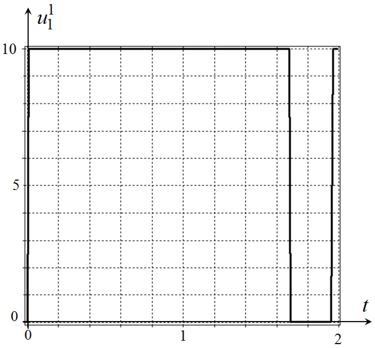
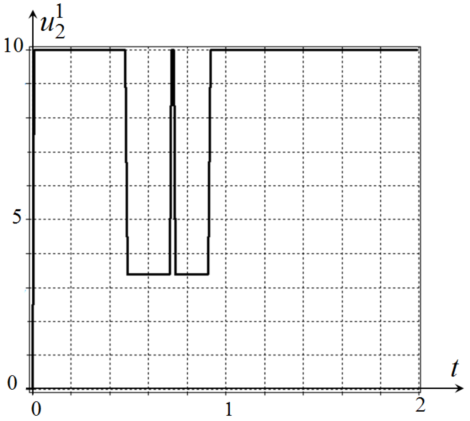
where $j=1,2$. Optimal control is calculated from equations

$${\tilde{u}}_1^j=\left\{\begin{array}{c}{u}_1^{j+},\mathrm{if}{W}_j+{\psi }_{3j}>0\hfill \\ u_1^{j-},\mathrm{if}{W}_j+{\psi }_{3j}<0\hfill \\ \mathrm{special}\mathrm{control}\mathrm{mode},\mathrm{if}{W}_j+{\psi }_{3j}=0\hfill \end{array}\right.,$$

(45)

$${\tilde{u}}_2^j=\left\{\begin{array}{c}{u}_2^{j+},\mathrm{if}{W}_j-{\psi }_{3j}>0\hfill \\ u_2^{j-},\mathrm{if}{W}_j-{\psi }_{3j}<0\hfill \\ \mathrm{special}\mathrm{control}\mathrm{mode},\mathrm{if}{W}_j-{\psi }_{3j}=0\hfill \end{array}\right.,$$

(46)

where

$$W_j={\psi }_{1+3(j-1)}sin{\theta }^j+{\psi }_{2+3(j-1)}cos{\theta }^j,$$

(47)

$u_1^{j+}$, $u_2^{j+}$, $u_1^{j-}$, $u_2^{j-}$ are upper and lower values of control for robot j, $j=1,2$.

The nonlinear programming problem consists of finding initial conditions for conjugate variables

$$q_i={\psi }_i\left(0\right),i=1,\dots ,6,$$

(48)

so that initial conditions have to allocate on a sphere with a unit radius

$$\sqrt{\sum _{i=1}^6{q}_i^2}=1,$$

(49)

as well as terminal time

$$t_f=t^{+}+q_7,$$

(50)

and special control modes

$$u_1^1=q_8,\mathrm{if}|W_1+{\psi }_3|<{\epsilon }_0,$$

(51)

$$u_2^1=q_9,\mathrm{if}|W_1-{\psi }_3|<{\epsilon }_0,$$

(52)

$$u_1^2=q_{10},\mathrm{if}|W_2+{\psi }_6|<{\epsilon }_0,$$

(53)

$$u_2^2=q_{11},\mathrm{if}|W_1-{\psi }_6|<{\epsilon }_0,$$

(54)

where ${\epsilon }_0$ is a small positive value.

A goal function for the nonlinear programming has the following form

$$F=\sum _{j=1}^2{\delta }_j\left(t_f\right)+a{\int }_0^{t_f}\sum _{j=1}^2{\mu }^2\left({\phi }_i(x^j,y^j)\right)dt+b{\int }_0^{t_f}{\mu }^2\left(\chi ({\mathbf{x}}^1,{\mathbf{x}}^2)\right)dt.$$

(55)

6. Computational Experiment

The problem had the following parameters: a number of objects $M=2$, dimensions of objects $n_1=3$, $n_2=3$, dimension of state space vector $n=3+3=6$, dimensions of control $m_1=2$, $m_2=2$, dimension of control space $m=2+2=4$ dimension of parameter vector $n+1+m=11$.

The following values of parameters of the algorithm were used: $x_0^1=0$, $y_0^1=0$, ${\theta }_0^1=0$, $x_0^2=10$, $y_0^2=10$, ${\theta }_0^2=0$, $x_f^1=10$, $y_f^1=10$, ${\theta }_f^1=0$, $x_f^2=0$, $y_f^2=0$, ${\theta }_f^2=0$, $u_i^{+}=10$, $u_i^{-}=-10$, $i=1,2$, $t^{+}=3.5$ s, $x_1^{*}=5$, $y_1^{*}=8$, $r_1=2$, $x_2^{*}=5$, $y_2^{*}=2$, $r_2=2$, $d=2$, ${\epsilon }_0=0.1$, $a=2$, $b=2$, $\epsilon =0.01$, $H=32$, $P=256$, $P_{length}=8$, $P_{rt}=0.33$, $∆=0.22$, $\beta =0.2$, $\alpha =0.3$, $K=7$, constraints on parameter values are $q_i^{-}=-1$, $q_i^{+}=1$, $i=1,\dots ,6$, $q_7^{-}=-2$, $q_7^{+}=1$, $q_i^{-}=-10$, $q_i^{+}=10$, $i=8,\dots ,11$.

An obtained optimal vector of parameters was

$$\mathbf{q}={[0.77220.2142-0.2825-0.2968-0.230.3702-1.51120.01793.3965-2.96-0.5945]}^T.$$

This solution provided the value of the goal function (55) $F=0.1238$.

To obtain the solution of optimal control problem for (33) and (44) by using the Pontryagin maximum principle, the complexity of search was the following: $H=32$, $P=256$, $R=H$, $P_{length}=8$, $step=0.22$, $n=8/0.22=36$, $H+nRP=32+36\times 32\times 256=294,944$, i.e., the functional was calculated 294,944 times. Simulation was performed in Lazarus, an open-source Free Pascal-based software, on PC with Intel Core i7, 2.8 GHz, OS Win 7. Series of 10 runs was implemented. The CPU time for 10 runs was approx. 20 min, i.e., 1 run was approx. 2 min.

The trajectories of the robots are shown in Figure 1. On Figure 1, red circles present the static constraints. Plots of obtained control are presented on Figure 2, Figure 3, Figure 4 and Figure 5. Figure 2, Figure 3, Figure 4 and Figure 5 show that optimal control includes sectors of special control modes [8]. The controls $u_2^1$ and $u_1^2$ have sliding modes.

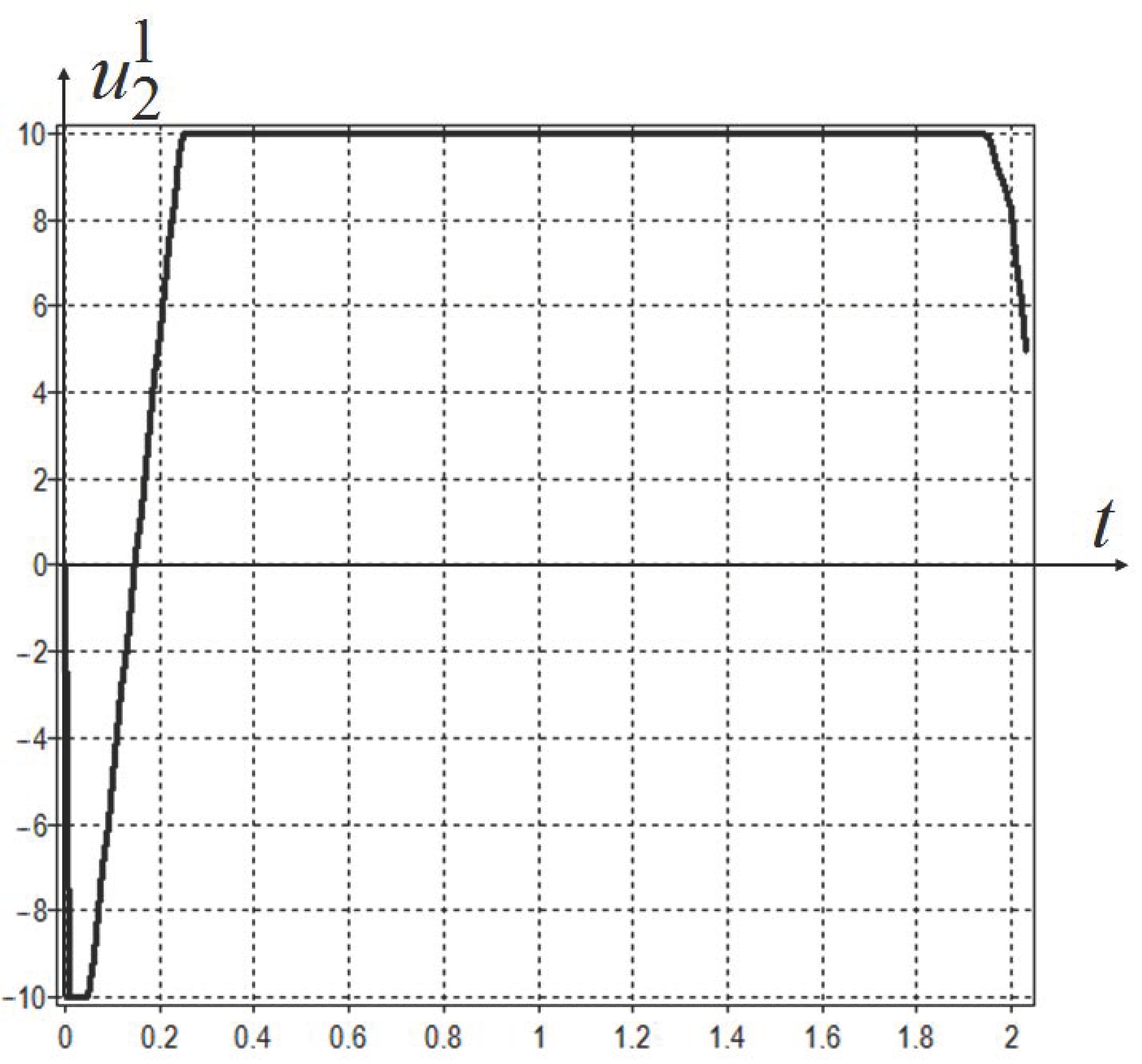
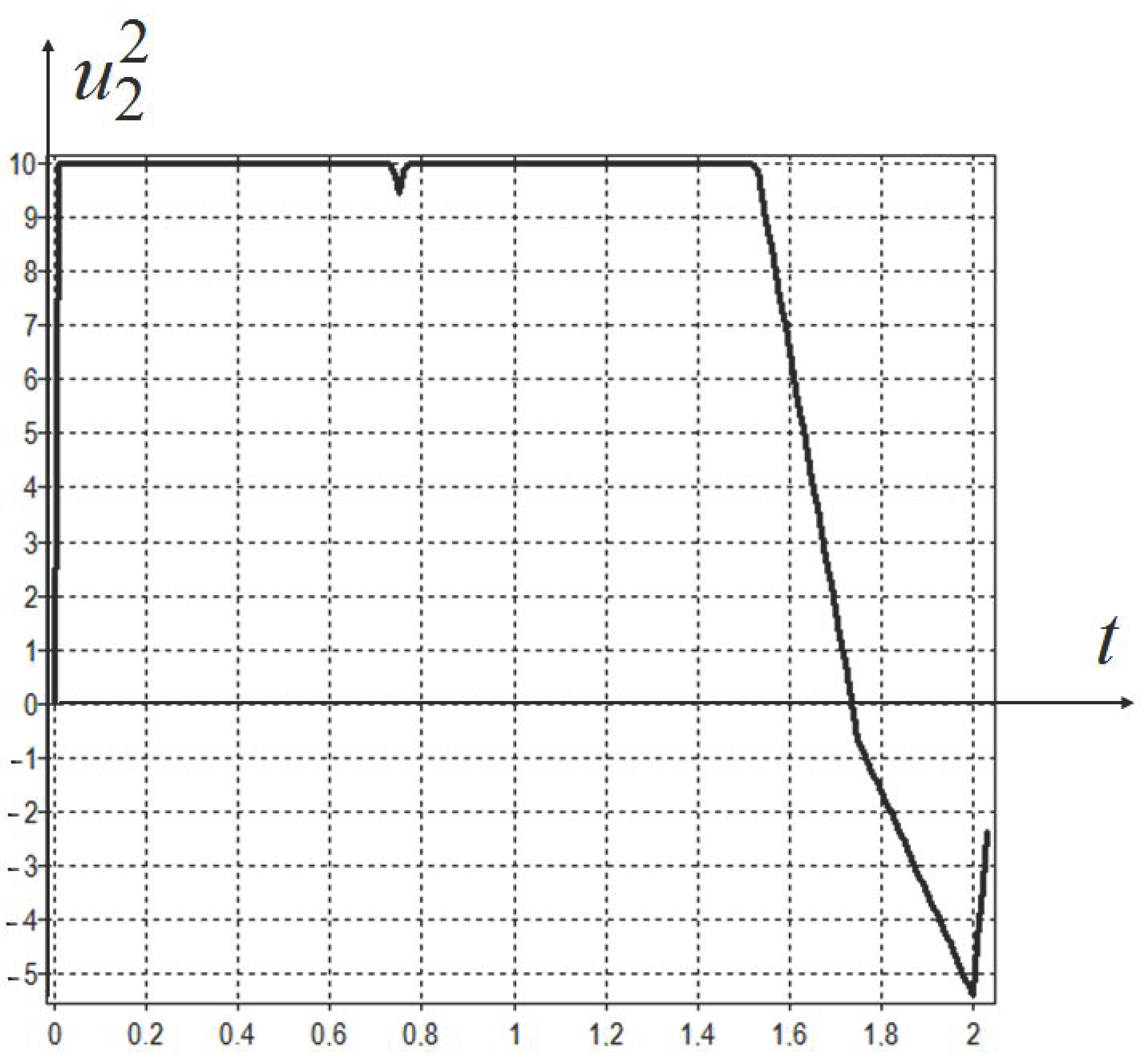
7. Search of Optimal Control by Direct Method

The same problem was solved by direct numerical method. Control for each robot was searched as a piece-wise liner function on interval as follows

$$u_i^j=\left\{\begin{array}{c}{u}_i^{+},\mathrm{if}{u}_i^{+}\le {\tilde{u}}_i^j\hfill \\ u_i^{-},\mathrm{if}{\tilde{u}}_i^j\le u_i^{-},\hfill \\ {\tilde{u}}_i^j,\mathrm{otherwise}\hfill \end{array}\right.$$

(56)

where

$${\tilde{u}}_1^1=q_i+(q_{i+1}-q_i)\frac{(t-i∆t)}{∆t},$$

(57)

$${\tilde{u}}_2^1=q_{i+K}+(q_{i+K+1}-q_{i+K})\frac{(t-i∆t)}{∆t},$$

(58)

$${\tilde{u}}_1^2=q_{i+2K}+(q_{i+2K+1}-q_{i+2K})\frac{(t-i∆t)}{∆t},$$

(59)

$${\tilde{u}}_2^2=q_{i+3K}+(q_{i+3K+1}-q_{i+3K})\frac{(t-i∆t)}{∆t},$$

(60)

$i=1,\dots ,K$, $t\in [i∆t;(i+1)∆t)$, $∆t=0.25$,

$$K=⌊\frac{t^{+}}{∆t}⌋+1=⌊\frac{2.5}{0.25}⌋+1=11,$$

(61)

Eleven time intervals were used. For each control, it was necessary to find 11 parameters of piece-wise linear function at the boundaries of intervals. Totally, we searched for forty-five parameters $\mathbf{q}={[q_1\dots q_{45}]}^T$, forty-four parameters were for control of two robots, and $q_{45}$ was for terminal time $t^{+}+q_{45}$. Values of parameters were constrained

$$q_i^{-}⩽q_i⩽q_i^{+},i=1,\dots ,45,$$

(62)

where $q_i^{-}=-20$, $q_i^{+}=20$, $i=1,\dots ,44$, $q_{45}^{-}=-0.8$, $q_{45}^{+}=0.8$.

The parameter search was also performed by modified SOMA. Vector of obtained parameters was as follows

$$\begin{array}{ccc}\hfill \mathbf{q}& =& [15.012917.468717.67722.253212.54889.00410.388619.999919.389919.01849\hfill \\ \hfill & & -8.8472-15.266910.516419.904416.572418.032817.559718.356316.86078,2100\hfill \\ \hfill & & -18.71274.3724-8.9377-0.793610.630918.966018.459718.974217.278114.6362\hfill \\ \hfill & & 18.4152-13.7367-2.852117.083718.175317.52789.461819.517817.600711.3479\hfill \\ \hfill & & {-0.6898-5.401519.92159.68500.6628]}^T.\hfill \end{array}$$

For direct approach, when we searched for 45 parameters by modified SOMA, the complexity of the algorithm was the following: $H=32$, $P=1024$, $R=H$, $P_{length}=8$, $step=0.22$, $n=8/0.22=36$, $H+nRP=32+36\times 32\times 1024=$ 1,179,680. Simulation was performed on PC with Intel Core i7, 2.8 GHz. A series of 10 runs was implemented. The CPU time for 10 runs was approx. 3 hours and 10 min, i.e., 1 run was approx. 19 min. We used $P=1024$ for direct approach, because the number of searched parameters was 45, and it was several times bigger than 11 parameters in the first experiment.

The obtained solution is presented on Figure 6. On Figure 7, Figure 8, Figure 9 and Figure 10, the plots of direct controls are presented.

8. An Alternative Non-Deterministic Control

One of the most important issues for swarm robotics applications is catching up with moving targets and avoiding multiple dynamic obstacles. It is complicated in that it requires an algorithm to work in real time to avoid obstacles that are standing or moving in an unknown environment, where the robot does not know their position until detecting them by sensors arranged on the robot. As an alternative to the method presented above, the use of swarm intelligence algorithms as reported in [9] can be discussed. The paper [9] presents a method for swarm robot to catch the moving target and to avoid multiple dynamic obstacles in the unknown environment. An imaginary map is built, representing N targets, M obstacles and N robots and a swarm intelligence algorithm is used to control them so that targets are captured correctly and in the shortest time. The robot dynamics can be viewed as a flow of water moving from high to low. The flow of water is the robot trajectory that is divided into a set of points created by an algorithm called SOMA [5,6]. Simulation results are also presented to show that the obstacle avoidance and catching target task can be reached using this method. All details about those experiments are discussed in [9]. Results are also visualized in selected videos (https://zelinkaivan65.wixsite.com/ivanzelinka/videa). The typical example is in Figure 11.

Besides the long-standing methods such as potential field method [10,11], and the vector field histogram [12], several new methods such as “follow the gap method” [13], and barrier function [14], or artificial intelligence methods such as genetic algorithm [15], neural network [16], and fuzzy logic [17,18] also demonstrate their effectiveness. Among the methods of artificial intelligence used to solve the problem as a function optimization problem, the self-organizing migrating algorithm (SOMA) emerges as a fast, powerful and efficient algorithm [5,6].

9. Discussion

The optimal control problem for two mobile robots with phase constraints was considered. To solve the problem, an approach based on the Pontryagin maximum principle was used. The mathematical model of robots include linear control in the right parts of differential equations; that is why the optimal control has sectors of special control modes. It should be noted that we used two robots to test the proposed technology and partially to test methodology. A larger group is required to fully test the proposed methodology and it will be our future research, but in the case of many robots, the optimization problem will go on backstage and the collision avoidance will become the real problem.

To solve a boundary-value problem and search of initial conditions of conjugate variables, the modified SOMA was used. Additional parameters for terminal conditions check and control in special modes were introduced.

The optimal control problem was also solved by direct approach. Control time was divided into intervals, and control at each interval was a piece-wise linear function. Additional parameter was also a time of terminal conditions check. The direct approach showed another character of objects movement.

The aim of this paper was to show for the first time how modern evolutionary algorithms can be applied to solution of boundary-value problems that occur when we solve the optimal control problem by an indirect method based on the Pontryagin maximum principle. Other known applications of evolutionary algorithms were mainly with direct approach [4].

Thus, one can conclude that the considered problem is multimodal and application of evolutionary algorithms to both direct and indirect approaches is expedient and prospective. The next research will be focused on an extensive comparative study of classical and swarm control based methods.

10. Patents

Certificate of software registration No.2020619668 Diveev A.I., Sofronova E.A. “Optimal control of group of robots based on Pontryagin maximum principle” 21 August 2020.

Certificate of software registration No.2020619960 Diveev A.I., Sofronova E.A. “Optimal control of group of robots by direct approach based on piece-wise linear approximation”, 26 August 2020.