1. Introduction
Model predictive control (MPC) is an optimal controller that minimizes a cost index over a finite horizon implemented in the receding horizon framework. The advantage of MPC over conventional controllers is the ability to handle the state and control constraints. When the state is measured at a sampling time, an optimization problem is solved. However, only the first element of the optimal solution is applied to the system. Then, the whole procedure is repeated at the next sampling time [
1].
The concept of a dual-mode MPC is widely used to guarantee the stability of MPC for both linear systems, e.g., [
2,
3], and nonlinear systems, e.g., [
4,
5,
6]. The terminal penalty function is used as an upper bound of the infinite horizon cost needed to drive the state trajectory to the origin when the initial condition is in the terminal region. Moreover, closed-loop stability is ensured by forcing the terminal state to belong to a feasible and invariant set. Hence, the region of attraction is the set of initial conditions that can be steered to the terminal region in
N steps or less, where
N is the prediction horizon. In other words, it is a
N-steps stabilizable set. Several studies have been devoted to formulate a terminal set that makes the region of attraction as large as possible. By increasing the prediction horizon, the domain of attraction can be enlarged at the expense of more computational effort due to the increasing number of decision variables [
7]. Hence, in the literature, various approaches have been proposed to enlarge the region of attraction through a larger terminal set. In [
8], it is shown that the saturated local control law is used to yield a considerably larger terminal constraint set. A sequence of sets is used in [
9] to replace a single terminal set. The contractive set does not need to be invariant as long as there is an admissible control that eventually steers the states to an invariant set. Hence, a larger domain of attraction can be obtained by extending the sequence with a reachable set. In [
10], the terminal constraint is only applied to the unstable states, giving the flexibility to have a larger set. A linear time-varying MPC is mostly used to extend a linear MPC with an enlarged terminal set for a nonlinear system, e.g., in [
11,
12,
13,
14].
Interpolation-based MPC for a linear system is studied by [
15,
16] to achieve a compromise between the size of domain attraction and the optimality. The MPC is designed by selecting several invariant sets and expressing the terminal state as a convex combination of states belonging to the invariant sets. By doing that, the resulting terminal set becomes the convex hull of the predefined-invariant sets. For reducing the number of decision variables, the interpolation method can be implicitly employed, meaning that the terminal state is not explicitly expressed as the convex combination of several states but is still the convex hull of several invariant sets, e.g., in [
17,
18]. The design procedure starts by designing several stabilizing feedback control gains
for a given linear time-invariant system. Then, feasible and invariant ellipsoids
,
, are defined such that some necessary linear matrix inequalities (LMIs) are satisfied for each matrix
. These LMIs are popularly used to show that
can be applied as the terminal set for a linear MPC [
19]. It is then shown that applying a convex combination to the
m given LMIs yields a new LMI. As a result, the set
is a feasible and invariant set for any
satisfying
. In view of this, the method used in [
17,
18] is highly dependant on the definition of the invariant sets through the use of an LMI form. Although an LMI form has been widely applied for many applications, e.g., in a consensus problem [
20,
21], the terminal set for a nonlinear MPC is not generally defined in an LMI form; thus, the convex hull may not be an invariant set despite that the ingredient sets
are invariant. To deal with this, a linear differential inclusion (LDI) is used in [
12,
13] to represent the nonlinear system. Specifically, the nonlinear system
can be represented as
where
and
with properly chosen
. As a result, after computing all ellipsoids using a common LDI, the convex hull of the several invariant sets can be used as the terminal set of a nonlinear MPC [
12]. However, LDI representation is generally conservative and is hard to obtain [
22]. With this in mind, this paper is interested in applying a more general convex combination to several terminal sets of a nonlinear MPC.
This paper aims to enlarge the domain of attraction of a nonlinear MPC by having a larger terminal region. Given several feasible and invariant sets , this paper proposes a convex combination strategy to define a new set to define a larger terminal set. The proposed strategy is different from the one discussed above as it does not require the help of LDI to make to be used as a terminal set for a nonlinear MPC. Moreover, it is shown that results in the union of . The feasibility and stability of the MPC can be guaranteed with the enlarged terminal set through the use of a common local Lyapunov function defined in all sets . Numerical simulations demonstrate that the proposed MPC has a larger region of attraction than the one obtained by the conventional MPC.
Notation
Given any sets and , the union and the convex hull of these sets are denoted by and , respectively. For a square matrix , denotes a positive definite matrix, and is the eigenvalue of A whose absolute value is smallest and is defined similarly.
2. Preliminary Result: Nonlinear MPC
Consider discrete-time nonlinear systems:
where
,
is the state and
is the input at time instant
k. The system is subject to the control input and state constraints
where
and
are convex and compact sets. It is assumed that the state
is measurable and there is neither external disturbance nor model uncertainty. The following assumption is required for system (
1).
Assumption 1. The function f is twice differentiable, and .
Having this assumption,
is an equilibrium of system (
1). The optimization problem for the finite horizon nonlinear MPC for nonlinear system (
1) is formulated as follows:
where
and
is the current state measurement. Here,
and
denote input and state predictions at time
that are computed at time
k. Thus,
is the control prediction over the prediction horizon. The function
is known as the terminal penalty cost. The matrix
and
are the weighting matrices for the state and input variables. Set
denotes the terminal penalty set where a popular choice for the terminal set is an ellipsoid set
, where
is a symmetric matrix.
The nonlinear MPC design procedure starts by solving the optimization problem when the state
is measured at the
kth sampling time. As a result, the optimal control sequence
is obtained, and
is applied to the plant. Therefore, the (implicit) model predictive control law is
. Afterward, the same procedure is repeated at the next sampling time. For details, see [
1,
5,
23].
Stability of MPC
The terminal region
and terminal penalty function
play a pivotal role in ensuring the stability of the nonlinear MPC (
3). The following lemma describes the required condition for stability.
Lemma 1. [1,3] With , , suppose that the following holds - A.1
such that , (feasibility)
- A.2
, (invariance)
- A.3
- A.4
.
Then, the origin is asymptotically stable for the closed loop system with a region of attraction , i.e., is the set of states steerable to by an admissible control in N steps or less.
For the purpose of enlarging the domain of attraction , this paper is interested in formulating an MPC in which its terminal set is defined as the convex combination of several invariant sets and is discussed in the next section.
3. MPC Based on the In-Between Terminal Set
In this paper, several sets are used as the ingredients of the time-varying terminal set for a nonlinear MPC. Specifically, given
m ellipsoids
, let
be an ellipsoid given by
where
and
. From (
5), a convex combination of
and
are used to define the new ellipsoid
. In [
24],
is called as the in-between ellipsoid. Note that
when
,
. Hence,
holds true, where
. In view of this,
in (
4) can be seen as a general way to define all
. A question arises on how the set
looks like. Note that
includes all the possible set
for any
such that
. In the following lemma, it is shown that
is a subset of the union of
.
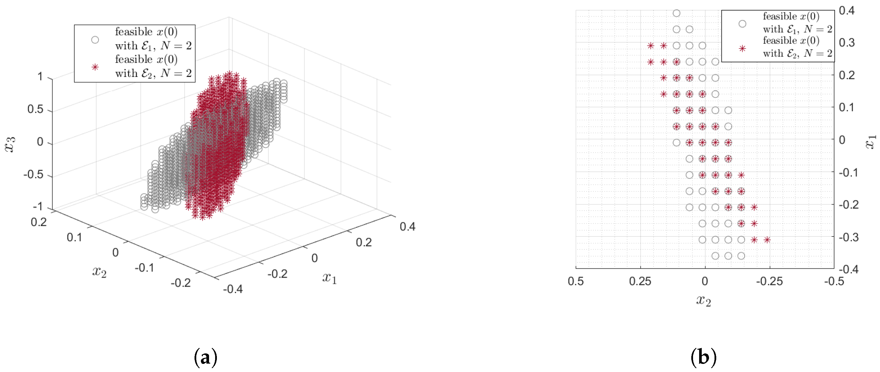
Lemma 2. in (
4)
is an ellipsoid satisfyingfor any satisfying . Since
when
and (
6) holds true, it follows that
, meaning that the union of all possible
results in the union of
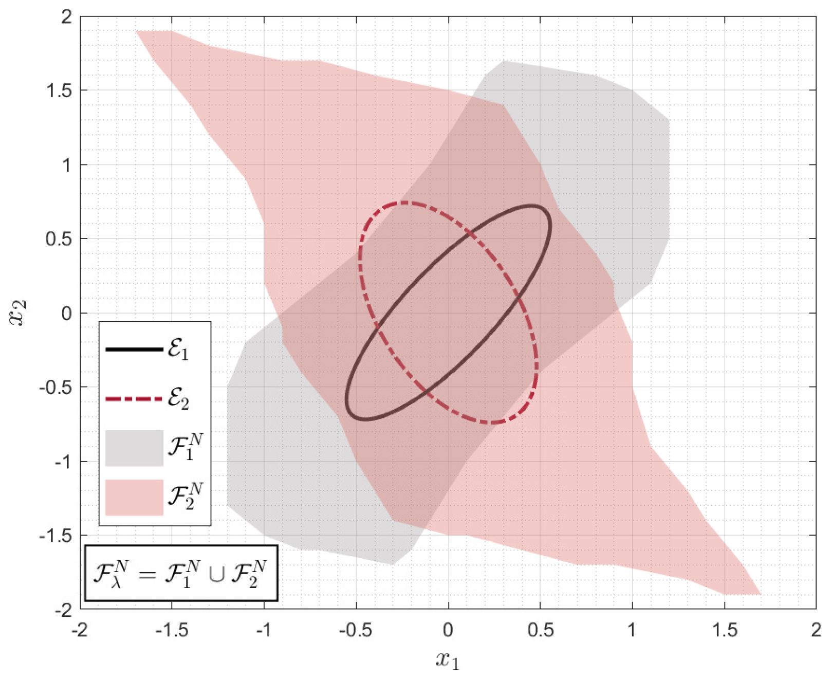
Figure 1 demonstrates Lemma 2 when only two ellipsoids
and
are considered. The property of
given by (
6) is depicted in
Figure 1b with
. It is important to note that convex combination (
5) does not result in convex hull of
as a convex hull is made by applying a convex combination of ellipsoids expressed by
with
[
17,
18]. See
Table 1. Instead, as can be seen in
Figure 1, the convex combination (
5) yields the union of
. Since, in general,
holds true, (
6) implies that
.Although this shows that the convex combination used in this paper results in a smaller set than the one obtained in [
17,
18], it is shown that under the following assumption, the in-between ellipsoid
can be used as the terminal set of an MPC and requires a relatively simple procedure even for nonlinear systems.
Assumption 2. For given and , suppose that there exist m pairs of satisfying A.1-A.3 of Lemma 1, and such thatwhere is a symmetric and positive definite matrix and . In the literature, there are several methods to find an invariant set and a terminal penalty cost such that the stability of the quasi-infinite horizon-based MPC (
3) can be guaranteed, e.g., [
5,
25,
26]. In these studies,
is shown as a local Lyapunov function in the set
under a stabilizing control law
, meaning that A1-A4 in Lemma 1 are satisfied. Thus,
and
can be used as the terminal penalty and the terminal region of a nonlinear MPC, respectively. However, Assumption 2 requires the existence of a common local Lyapunov function
defined in all the sets
[
27]. Suppose that
satisfying Lemma 1 are given in the first place, the common Lyapunov function can be found by choosing a positive definite matrix
such that the following holds true
Note that (
8) is equivalent with (
7). A method based on the existing method [
5,
25,
26] can also be employed to make Assumption 2 holds true. In fact, the following lemma can be obtained by extending the result in [
26].
Lemma 3. Suppose that Assumption 1 holds true, and that the following linearized system of (
1)
in the neighborhood of the origin is controllableLet be a stabilizing feedback control law with feedback gain K and P be a positive definite matrix satisfyingwhere , . Moreover, suppose that is a positive definite matrix such thatThen, there exists a constant α specifying an ellipsoid in the form of such that , , is an invariant set for nonlinear system (
1)
, and that the following holds true Having this lemma, the sets
satisfying Assumption 2 can be obtained through the use of the linearized system and state feedback control laws. Specifically,
is chosen such that (
11) holds true for the given
, and
is chosen such that (
12) holds true. The details of the method and the proof of the lemma are given in
Appendix B.
Given
, the proposed MPC with enlarged terminal region is computed by solving the following optimization problem
where
,
and
. In the following, it is shown that the stability of the proposed MPC computed by (
13) can be guaranteed.
Theorem 4. For the nonlinear system (
1)
, suppose that Assumptions 1 and 2 hold true, and that the optimization problem (
13)
with and is initially feasible. Then, the closed-loop system consisting of the system (
1)
and the nonlinear MPC obtained from (
13)
is asymptotically stable. Proof. Let
, and
,
, be the optimal solution of problem (
13) at time
k. Then, the optimal vector
and
are given by
Having this, the optimal cost function at time
k is given by
By Lemma 2, there is at least one
j,
, such that
. Note that
,
, are feasible at
since
is an invariant set with
. Thus, the following is a feasible control sequence at
The resulting state prediction is given by
where
due to the invariant set
. Using (
15) and (
16), the cost function at
is
Note that
is not the optimal cost function at
. Moreover, (
17) can be rewritten as follows
where
is defined in (
14). Applying (
7) to this inequality yields
As a result, the optimal cost function at time
, denoted by
, satisfies
In other words, the optimal cost function is a Lyapunov function for system (
1). Having this and the terminal state constraint, nonlinear system (
1) under the solution of (
13) is asymptotically stable at the origin. □
Note that optimization problem (
13) uses
as the fixed penalty cost function but employs a time-varying terminal set
. Since
can be any non-negative constants such that their sum is one, the union of
can be seen as the terminal set of (
13), meaning that the proposed method potentially yields larger region of attraction when the region of attraction of each invariant set
is not the subset of the others, i.e.,
.
Although the resulting terminal set is not the convex hull of the predefined sets, the proposed method can be easily employed for a nonlinear system without the need for an LDI argument. Moreover, the ingredient sets
can be obtained using a similar procedure as in [
5,
25], or [
26]. In the next section, numerical simulations are used to investigate the performance of the proposed MPC for a nonlinear system.


