Advances in Tracking Control for Piezoelectric Actuators Using Fuzzy Logic and Hammerstein-Wiener Compensation

Abstract

Piezoelectric actuators (PEA) are devices that are used for nano- microdisplacement due to their high precision, but one of the major issues is the non-linearity phenomena caused by the hysteresis effect, which diminishes the positioning performance. This study presents a novel control structure in order to reduce the hysteresis effect and increase the PEA performance by using a fuzzy logic control (FLC) combined with a Hammerstein–Wiener (HW) black-box mapping as a feedforward (FF) compensation. In this research, a proportional-integral-derivative (PID) was contrasted with an FLC. From this comparison, the most accurate was taken and tested with a complex structure with HW-FF to verify the accuracy with the increment of complexity. All of the structures were implemented in a dSpace platform to control a commercial Thorlabs PEA. The tests have shown that an FLC combined with HW was the most accurate, since the FF compensate the hysteresis and the FLC reduced the errors; the integral of the absolute error (IAE), the root-mean-square error (RMSE), and relative root-mean-square-error (RRMSE) for this case were reduced by several magnitude orders when compared to the feedback structures. As a conclusion, a complex structure with a novel combination of FLC and HW-FF provided an increment in the accuracy for a high-precision PEA.

1. Introduction

Smart materials, like piezoelectric, are widely used in systems where nano- microdisplacement and precision are required [1,2]. Piezoelectric actuators (PEAs) are derived from this technology, where not only can they provide high-precision at small displacements, but also support high forces in comparison to their size [3]; these properties are advantageous due to the downsizing needed for actuators nowadays [4]. PEAs are also designed and produced in different degrees of freedom (DOF), which depend on the required application [5]; a vast number of uses for these actuators, such as computer components [6], machine tools [7], energy recovery [8], and micro-drones [9], are available. Furthermore, PEAs are also used in medicine, where precision is extremely important for purposes as cell puncture [10], drug delivery systems [11], and needle positioning for complex injections [12].

Nonetheless, the demeanour of PEA contains non-linearities. like vibration dynamics, creep, and hysteresis, which yields undesirable operation [13]. Vibration dynamics are caused by the input voltage excitation that operates the equivalent mechanical system, although this should be considered when the input frequency reaches the resonance of the PEA [14]. Creep represents an effect that is produced by the polarization that remains in time during the actuation in a quasi-static situation [15]. The hysteresis is provoked by the non-linear piezoelectric effect in combination with the mechanical action and electric field [16].

The hysteresis has not only has been studied in electromagnetic materials [17], but also in PEAs positioning due to adverse causes in the accuracy and margins of stability [18]; usually, the error inaccuracy can be up to 22% in an open-loop configuration [19]. The microscopic origin and theory of hysteresis in PEAs are complex, although an explanation in [20] shows that this feature is associated to the irreversible restoration of the unit cells when the electric field is reduced; on the other hand, ref. [16] encompass the theory with the movement of the domain walls. Certainly, for these reasons, the hysteresis not only depends on the presently applied input, but also in the previous input schedule [21]. Despite the natural origin of hysteresis, where elimination is inconceivable, it can be diminished while using a suitable control strategy in order to achieve an ultra-precision in the guidance.

The decline of hysteresis can be done via an advanced control strategy. Feedforward (FF) compensation aims to map the non-linearity of the device in order to compensate for the phenomena; it has been demonstrated that when the PEA is unloaded, FF is effective [22]. However, the error reduction, dynamic changes, and unknown effects are properties in which FF fails to compensate, but where a feedback strategy can deal with. The latter mentioned offers a solution that can increase the precision, although the close-loop can result in a low gain margin that narrows the use of high-gain controllers [13].

Despite the drawbacks of the mentioned strategies, a combination of both frameworks can be a suitable option to analyse. Feedforward-feedback controllers can increase the control accuracy of PEAs through the advantages that both techniques can provide separately [23]; furthermore, this strategy can produce multiple structure combinations. In [24], the hysteresis was compensated with a linear and artificial neural network (ANN) combined with a conventional proportional-integral-derivative (PID) and a neural type; results shown that the combination of ANN with the neural PID has been the most precise one, since the integral of the absolute error (IAE) was reduced to 0.049. The authors of [25] described the FF compensation by a Prandtl–Ishlinskii hysteresis model merged with sliding mode control (SMC) as feedback; results unveiled an error less than 1%. Another solution was presented by [26], where a polynomial based approach mapped the hysteresis curve for FF and combined with a PID control; the results have shown a precision increment, although the deviation was also significant. Another advance strategy was used in [27], where the authors employed a mathematical based model, such as Dhal, merged with ${\mu }_{\infty }$, which provided an error of 0.51%. However, these structures have certain drawbacks as computational requirements in the case of ANNs training, time-consumption to achieve a suitable model when a FF was used, or complexity implementation as the preceding explained example.

Fuzzy logic control (FLC) is a structure that mimics human knowledge or action based on linguistic rules that are tuned according to the designer [28,29,30]; these type of controllers have been used in applications for maximum power point tracking, such as fuel cells and photo-voltaic systems [31,32], electrical drivers [33], etc. The author of [34] indicated that FLC that is based on PID grants a high accuracy for PEAs guidancem, but it can also provide other advantages over alternative control structures. The authors of [35] compared an $H_{\infty }$, which is a robust controller already used in PEAs [36], with a FLC for a tracking problem; the results displayed a superior performance in terms of the steady-state error and overshoot. On the other hand, SMC is another well-used framework for PEAs [37]; however, the researchers from [38] encourage the use of FLC over SMC due to its practicality and no chattering effect.

In this research, a type-1 FLC based on PID was used; according to [39], this kind of structure tends to perform better than a conventional PID, since it handles uncertainties that are related to the controller input and output, operational changes, and disturbances through rules and the fuzzifier. In combination with the FLC and to improve the uncertainty, analytic methods could have been used, although certain disadvantages were taken into account. Bouc–Wen is an efficient hysteresis model that could be merged as FF; however, its performance decreases when the non-linearity shows asymmetry [40]. Another option is Prandtl–Ishlinksii model, which is widely used; however, its inversion is complex, and it could increase the error compensation [41].

Black-box (BB) models are a block based approach that provide a mapping between the input and the output, but without taking the physical relations of the system into account [42]. Hammerstein–Wiener (HW) is an advance BB where the shape consists of a linear representation followed and preceded by non-linear blocks. This identification tool is widely used in non-linear systems, such as chemical reactors [43], voltage distortion of batteries [44], and motion precision of electro-mechanical systems [45].

The structure of this paper is organized, as follows: Section 2 provides an overview of the hardware that was used in the research, a brief description of the hysteresis, and an explanation about how the HW block works. Section 2.3 resumes the control structures which were involved: in this investigation, a PID, a type-1-FLC and a type-1 FLC-HW were used and compared. Section 3 presents the results in two steps, where the PI and type-1-FLC were compared as feedback controllers and the one that had performed best was contrasted in the following subsection with a complex FF with HW and FLC to grasp the contribution in terms of performance. Finally, Section 4 concludes and analyses the results of the work done along with the research.

2. Materials and Methods

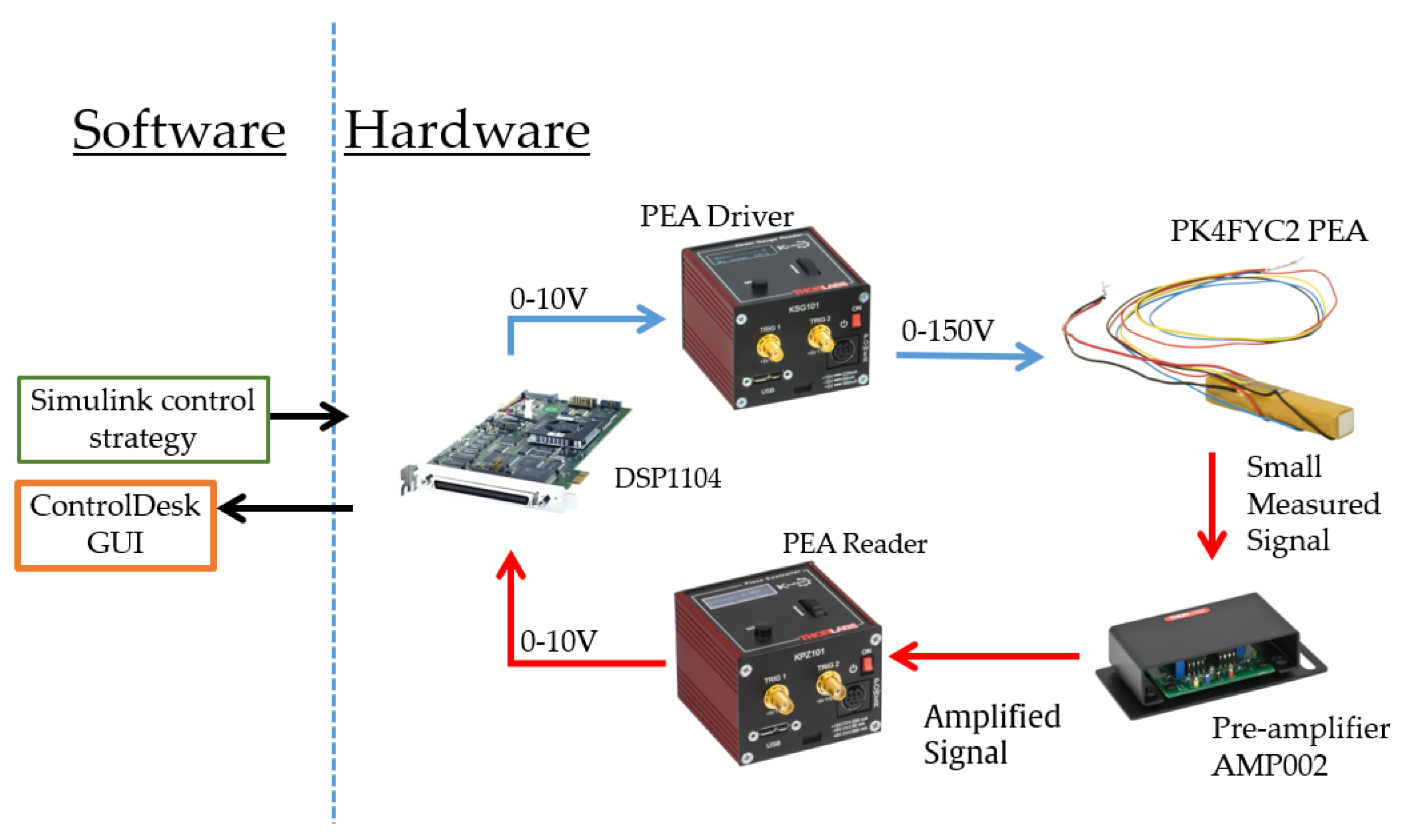
Figure 1 shows the framework implemented for hardware and software, where a commercial Thorlabs PK4FYC2 PEA was used, which is a stack actuator that consists of multiple chips stick with epoxy and glass beads; the measurement of displacement is acquired with a four attached metal foil strain gauges that are configured as a Wheatstone bridge circuit. At the maximum drive voltage (150 V), the displacement is 38.5 $\mathsf{\mu }$m with a hysteresis that can produce up to 15% of error. The actuator has a length of 36 mm and squared transverse section with a length of 7.3 mm. The maximum force that the device can support is 1000 N and the resonant frequency is 34 kHz.

The ancillary equipment consisted of a pre-amplifier Thorlabs AMP002, a measurement cube reader Thorlabs KSG101, a driver cube Thorlabs KPZ101 (which works in open and close loop operation), and controller board dSpace DSP1104. The hardware was configured so that the DSPS1104 could generate an analog signal of 0–10 V and sent to the KPZ101 that magnified into 0–150 V for the PEA actuation. As a result, the strain gauge could monitor the displacement of the PEA and this signal was augmented through the AMP002, which was afterward sent to the KSG101 and scaled in a 0–10V signal, which is the input range that the DSP1104 could acquire.

As means to the software architecture, Simulink by Mathworks was used in order to design the control frameworks; System Identification Toolbox was used for the FF and FLC Toolbox for the feedback. The data acquisition, supervision, and tuning of the parameters was done in a graphical user interface through ControlDesk, which belongs to dSpace. Finally, due to the relation of hardware limitation versus data acquisition, the sampling time was defined as 1 kHz.

2.1. Hysteresis Description and Reference Design

A hysteresis graph can be obtained using sine or triangular waves in time as an input and as post-processing, the generation of a plot of input voltage versus displacement. The triangle wave is a complex source as a reference, since it consists of high-frequency harmonics that can raise the tracking difficulty, according to [46]. Thus, a triangle wave was used to obtain the hysteresis graph and as a reference for guidance, a configuration as in [24] where the period chosen was 2 s with a maximum amplitude of 150 V, since, at the utmost driving voltage, the non-linearity analysed has its maximum reflection.

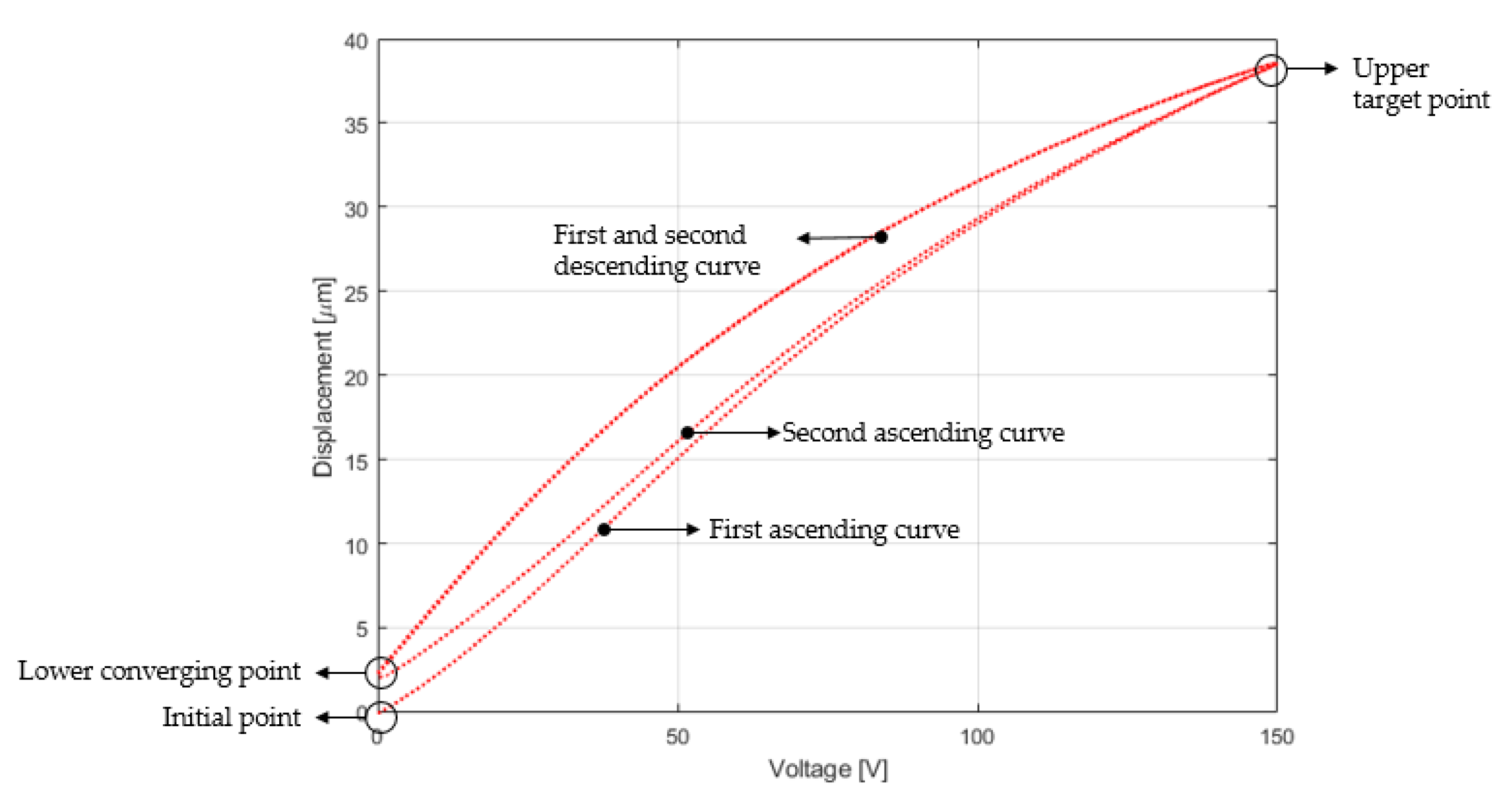
Figure 2 is the PK4FYC2 hysteresis graph for two triangle cycles, where the first ascending curve has its initial point that begins at the origin or also called Initial point and ends at the Upper target point. Provided that the amplitude and frequency of the input do not change [24], this demeanour only occurs for the first rising curve, since the following cycles converge to a single hysteresis curve, where the lower converging point and the upper target point will be permanent. According to this analysis, the conversion from voltage to displacement for reference design cannot be done by multiplying the maximum displacement divided by the maximum voltage which implies a straight line between the initial point and the upper target point. Therefore, a realistic approach is the usage of a straight line as a reference path, where Displacement [$\mathsf{\mu }$m] = m*Voltage [V] + c, where m is 38.5 − c $\mathsf{\mu }$m/150 V and c is the vertical offset of the lower converging point.

2.2. Hammerstein-Wiener Model

As previously seen, the hysteresis is highly non-linear not only because there are two different values for a voltage, but also an asymmetry is present that can be difficult to represent with an analytical method. Hence, a mapping strategy should be designed to trim the phenomena because there can be two values of voltage for a single reference point. According to [47], Hammerstein blocks are used when the input behaves with significant non-linearity; thus, the input $u\left(t\right)$ is transformed by a non-linear function f, which is then multiplied by a linear transfer function B/F. Conversely, the Wiener block uses a non-linear function h, where the arguments are the input signal multiplied by the linear transfer function and results in an output y(t). The conjunction between both theories (Hammerstein–Wiener) results in a three-block step that maps systems with strong non-linearities in the inputs as in the outputs. The fringes of HW which correspond to the non-linear functions f and h can be approximated with different methods such as piece-wise linear functions, sigmoid, dead-band, wavelet, and polynomial. A summary of these theories is mathematically expressed in Equation (1).

Equation (2) is the linear subsystem B/F, where $n_b$, $n_f$, and $n_d$ denote, respectively, the degree of B, F and the associated delay. This transfer function is expressed in the time shift operator $q^{-1}$, which represents $q^{-1}u\left(t\right)=u(t-T)$, where u(t) is the system input and T is the sample time. The coefficients that correspond with the three functions can be obtained using real the data of the PEA.

$$\left\{\begin{array}{c}\mathrm{Hammerstein}\mathrm{block}\Rightarrow y\left(t\right)=f\left(u\left(t\right)\right)x\left(q^{-1}\right)\hfill \\ \mathrm{Wiener}\mathrm{block}\Rightarrow y\left(t\right)=h\left(x\left(q^{-1}\right)\right)\hfill \\ \mathrm{HW}\Rightarrow y\left(t\right)=h\left(f\left(u\left(t\right)\right)x\left(q^{-1}\right)\right)\hfill \end{array}\right.$$

(1)

$$x\left(q^{-1}\right)=q^{-n_d}\frac{B}{F}=q^{-n_d}\frac{{\sum }_{i=1}^{n_b}{b}_i{q}^{-i+1}}{1+{\sum }_{j=1}^{n_f}{b}_j{q}^{-j}}$$

(2)

The MATLAB System Identification Toolbox was used in order to estimate the parameters of HW block; the software approximates the input and output nonlinearities using a loss function as a first metric in order to reduce the error between the model output and response measured. The iteration algorithm was set into automatic choice, so that the software can search the adequate one. The second metric that was taken into account was the Fit Percent, which is related to “how good the model fits the experimental data”, and it varies from $-\infty$ to 100, which represents, respectively, the lowest and highest fitting accuracy. This metric is expressed as Equation (3) shows, where $y_{measured}$ is the measured output data, $\overline{y_{measured}}$ is its mean and $y_{model}$ is the predicted response of the model.

$$FitPercent=100\left(1-\frac{\left|\right|y_{measured}-y_{model}\left|\right|}{\left|\right|y_{measured}-\overline{y_{measured}}\left|\right|}\right)$$

(3)

2.3. Feedback Control Design

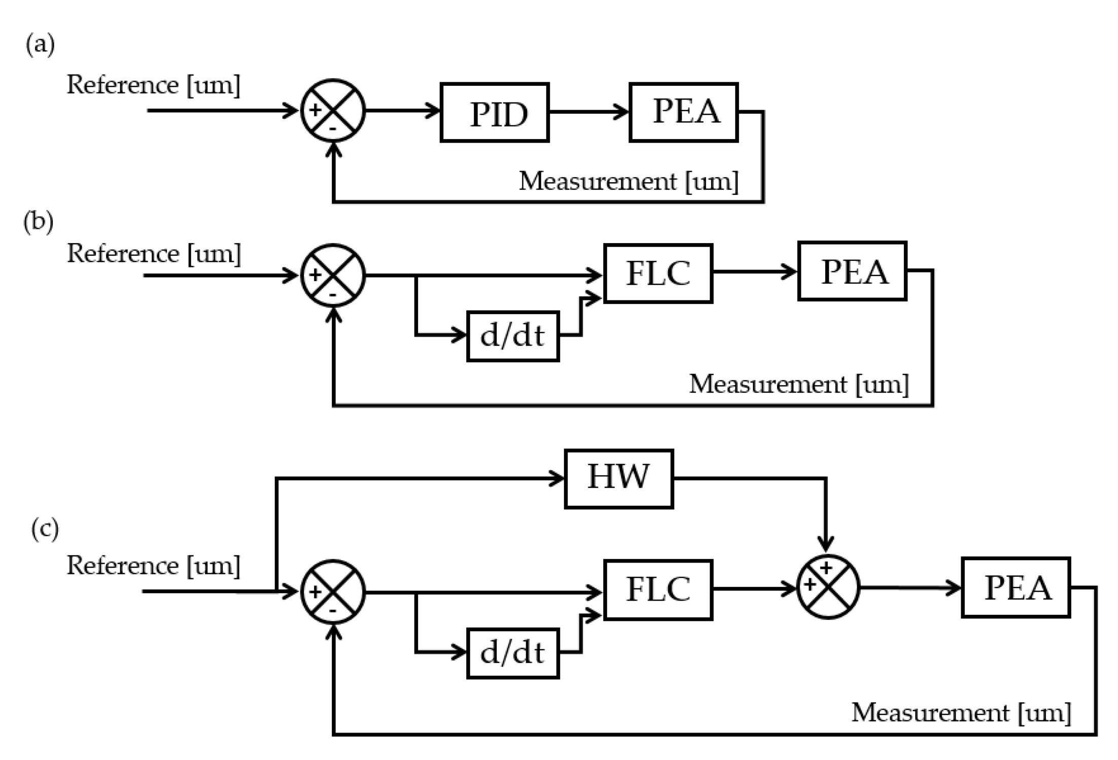
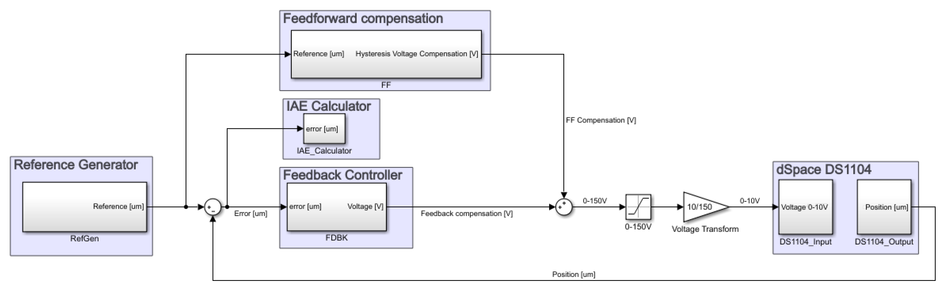
The comparison was undertaken with three different types of control frameworks in order to verify their performance. The progression criterion of the test was done from a simple to a complex structure, where each controller was embedded into the hardware previously described. Figure 3 shows these configurations that were embedded in Simulink (Figure 4 shows the complex structure embedded as an example). The contrast of results, which will be presented in the following sections, was made in two groups: in a first step, feedback controllers (PID and FLC) were analysed and the one that behaved better was picked for an ultimate comparison with the complex architecture (FLC with HW), since it was expected to exceed due to the FF compensation.

Since all three structures had gains to be tuned, the IAE was used in order to achieve the best performance. Equation (4) defines this metric where e(t) represents the error and that resembles a perceptive expression for positive and negative values.

$$IAE={\int }_0^{\infty }\left|e\left(t\right)\right|dt$$

(4)

Additionaly, in order to quantify the performance of the control frameworks, the root-mean-square error (RMSE) and relative root-mean-square-error (RMSE) were calculated for the tracking signals. The expressions of these metrics are shown in Equations (5) and (6), where $e_i$ and $r_i$, respectively, the error and the reference at the i-th sample, the length of the sampling data and the reference trajectory; N represents the length of the analysed data.

$$RMSE=\sqrt{\frac{1}{N}\sum _{i=1}^N{\left(e_i\right)}^2}$$

(5)

$$RMSE=\sqrt{\sum _{i=1}^N{\left(e_i\right)}^2/\sum _{i=1}^N\left(r_i\right)}\times 100\%$$

(6)

2.3.1. PID Control

A simple structure, like PID, can be a suitable launch for many systems to be controlled and, since the FLC used in this research is based on a PID, a comparison with a conventional controller is fair for contrasting the performance. The classical expression from Equation (7) was embedded in Simulink and tuned while taking into account the values that can drive the system to an unstable or unsuitable performance as well as reducing the IAE. The terms $K_p$, $K_i$, and $K_d$ are the tuning parameters that correspond to the proportional, integral, and derivative, which were settled by the reduction of the IAE that depends on the error e(k).

$$u\left(k\right)=K_{p}e\left(k\right)+K_i\sum _{i=1}^{k}e\left(i\right)\Delta t+\frac{K_d[e\left(k\right)-e(k-1)]}{\Delta t}$$

(7)

2.3.2. Type-1 Fuzzy Control

If the error value is positive and large with a positive increase, then a big control effort needs to be applied considering that its magnitude should shrink as the error is reaching the zero so that overshoots can be avoided, as was experimentally observed. It was considered that with negative values the situation is symmetric.

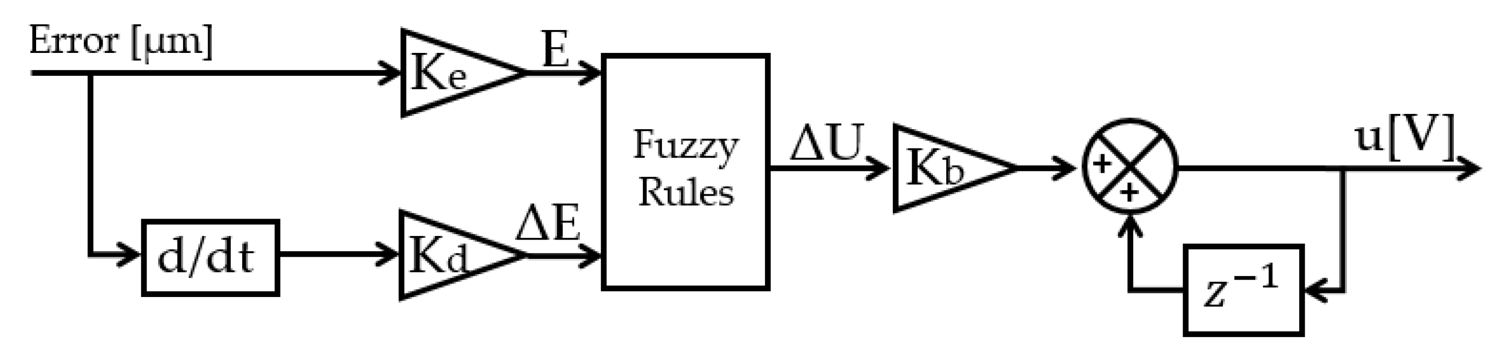
An improved procedure from the last presented architecture is a type-1 fuzzy interference, which is a non-linear controller that operates better than a conventional PID, especially for severe nonlinearities [39]. The input to the controller consists of the error and its derivative that are multiplied by the factors $K_e$ and $K_d$; this results in the variables E and $\Delta$E, which represent error and its change normalized in the range of [$-1$ 1]. The constant $K_b$ is intended to increase the output of the FLC based on an incremental control action (Figure 5).

The structure of the rules was configured, as the Equation (8), where $\Delta$U is the output of the fuzzy block, $G_m$ is the corresponding crisp set in which m goes from 1 to the total number of rules used; k and l cover the range of membership functions that corresponds to E and $\Delta E$, respectively. The fuzzification process entails triangular overlapped membership functions that are related to each normalized input. In this research, the membership functions for the inputs were uniformly discretized in terms of negative big (NB), negative medium (NM), negative small (NS), zero (Z), positive small (PS), positive medium (PM), and positive big (PB); these values were defined as $-1$, $-0.66$, $-0.33$, 0, 0.33, 0.66, and 1, respectively. Therefore, 25 fuzzy rules were adapted, where its defuzzification mechanism was configured in constants discretized uniformly in the range of [$-1$ 1].

$$R_m:\mathit{If}E=B_{1k}\mathrm{and}\Delta E=B_{2l}\Rightarrow \Delta U=G_m$$

(8)

This controller was tested under two frameworks: first, as a feedback structure and, secondly, the HW was added as an FF. The gains had to be different in both cases, since, with the same values, the comparison would have had a significant gap in terms of error. Figure 3b presents a feedback control with FLC that has the role of suppressing errors, alteration of the PEA dynamics, or unknown uncertainties. Figure 3c displays the same structure, but with an FF that pretends to compensate the non-linear effects with an HW model.

2.3.3. FLC Stability Proof

Although the scope of the current article is to provide experimental results for PEA tracking performance, a semi-formal stability proof is presented based on the Lyapunov theory of stability [48]: if a dynamical system is asymptotically stable, then there exists a positive definite Lyapunov function V: $R^n\to R$, so that $V\left(x\right)>0$, $V(\infty )=\infty$, $V\left(0\right)=0$ & $\dot{V}\left(x\right)<0,\forall x\ne 0$,. Therefore, if the normalized error is defined as $E=X_{ref}-X$, then a Lyapunov function is defined as Equation (9).

$$V=\frac{1}{2}{E}^2$$

(9)

$$\dot{V}=E\dot{E}$$

(10)

Thus, if the derivative (Equation (10)) of the Lyapunov function is negative, then it implies that the system is asymptotically stable and it converges to a null error. Considering when the control signal $\Delta$U is positive, then $\Delta$X is positive and $\Delta$E is negative, which implies that $\dot{E}<0$. In the same way, when $\Delta$U is negative, $\Delta$X is negative, which yields to a positive $\Delta$E and, hence, $\dot{E}>0$. Therefore, linguistic rules are analysed, as follows:

• Case 1: if E is PS or PB and $\Delta$E is PB, PS or Z | E is PB and $\Delta$ E is NS | E is Z and $\Delta$E is PB or PS $\Rightarrow U=PS$, PM or PB.

During this situation, the increment of $\Delta$U drives to $\dot{E}<0$ with a positive E and, hence, the error converges to the null value because $\dot{V}<0$

• Case 2: if E is PS and $\Delta$E is NB | E is NS and $\Delta$E is PB $\Rightarrow U=Z$.

In this condition, the signal $\Delta$U is null and it means that the feedback control signal does not change, so that the $\dot{V}<0$, although the trend stills tends the error to a null value due to the sign of $\Delta$E.

• Case 3: if E is NB or NS and $\Delta$E is NS, NB, or Z | E is NB and $\Delta$E is PS | E is Z and $\Delta$E is NB or NS $\Rightarrow U=NS$, NM or NB.

Reciprocally to case 1, when $E<0$ and $\dot{E}<0$, which is switched to a positive value, since $\Delta$U decreases; thus, this yields the error to converge to a zero value.

For the rest of the linguistic rules, which are the cases of the diagonal of

Table 1. FLC linguistic rules.

E$\setminus \mathbf{\Delta }$E	NB	NS	Z	PS	PB
NB	NB	NM	NM	NS	Z
NS	NM	NM	NS	Z	Z
Z	NM	NS	Z	PS	PM
PS	Z	Z	PS	PM	PM
PB	Z	PS	PM	PM	PB

, the Lyapunov stability is verified, since, at each moment, $\dot{V}<0$, and the error tends to decrease due to the demeanour of E and $\dot{E}$.

3. Results and Discussion

3.1. Hammerstein-Wiener Training Results

The different options of approximators for the non-linear blocks were tested in order to find the best solution in terms of the fit percentage. The results provided a fit percentage of 99.58, 93.33, 91.02, 96, and 99.57, which correspond with a piece-wise, sigmoid, dead-zone, wavelet, and polynomial, respectively. Therefore, the piece-wise had the best fit-percentage, which works, as follows: within the chosen inputs and outputs, there are breakpoints that are associated ($x_i$, $y_i$) such that i = 1 … n so $y_i$ = R($x_i$), where n is the number of breakpoints (input or output), R is the piece-wise function that is approximated through the breakpoints, where $x_i$ and $y_i$ are obtained by the algorithm previously explained.

3.2. Hysteresis Fitting Results

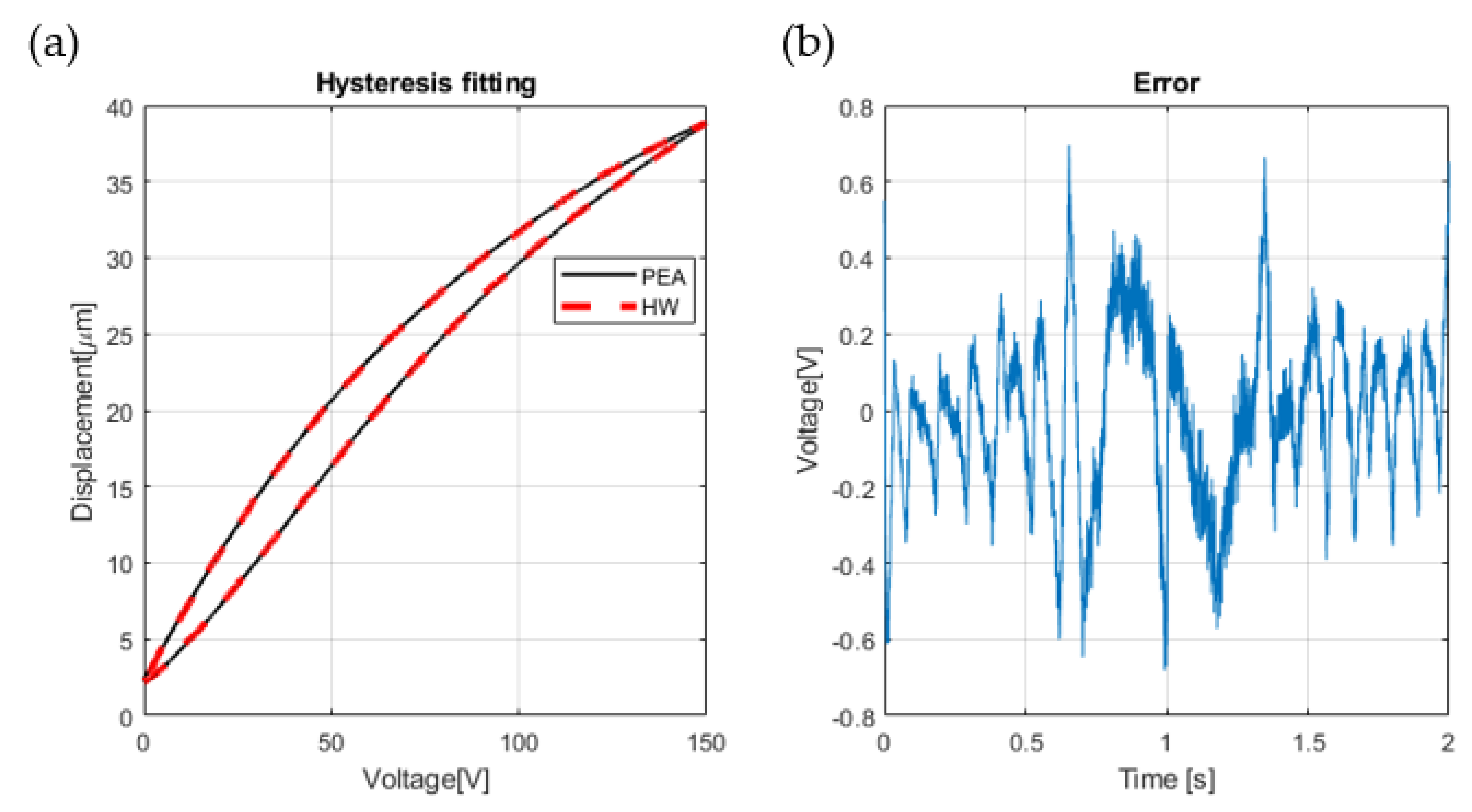
A first step before the control evaluation in feedback with FF structure is to test the mapping performance for achieving the tracking persistence. The HW was tested in a hysteresis graph to analyse the fitting of the model although the previous fit percent obtained was suitable. Because the input was expected to be the main reference so that the voltage was the output to be fed into the control system, the comparison was done in terms of the voltage error.

Figure 6a displays the fitting comparison of the HW model with the real data; Figure 6b is an associated error graph that displays the development of the fitting along one arbitrary cycle. The comparison shows an acceptable behaviour, since HW could manage to fit the hysteresis graph from the lower converging point up to the upper converging point, as well as the asymmetry feature that this PEA has. Moreover, the error graph augments the previously described manner, where it can be seen that the magnitude fluctuates between $-1$ and 1 V; a harsh demeanour occurs at 1 s, which is the moment where the input changes its slope to decrease and, thus, this was an expected unfolding due to the complex alteration.

3.3. Tracking Control Results

The three control architectures were embedded in the hardware distribution that was presented in Figure 1. The first was a PID as feedback without FF compensation, the second FLC in feedback, and finally, FLC combined with HW-FF. The comparisons were performed in two groups by separately comparing feedback controllers to inspect the performance and emphasize the best feature of each; from this contrast, the best one was analysed against the complex structure, the FLC with HW-FF.

As previously seen, all of the controllers had gains to be tuned, which were obtained by reduction of the IAE so as to pursue the maximum performance. Regarding the FLC, since the input to the rules block is between [$-1$ 1], this was also monitored, so that the controller behaviour could be suitable. Furthermore, it was taken into account the limits of the PEA input voltage by implementing saturations to prevent critical situations for the device.

The gains that were obtained for the PID controller were 10, 1000 and 0 for the $K_p$, $K_i$, and $K_d$, respectively. The parameters for the FLC in close loop mode were set as 16.2, 0.008, and 0.8 which correspond, respectively, to $K_e$, $K_d$, and $K_b$. Finally, to improve the performance, the constants of the FLC with HW-FF were switched, so that the obtained values were 4.2, 0.006, and 0.8, which correlate with $K_e$, $K_d$, and $K_b$.

3.4. PID vs. FLC

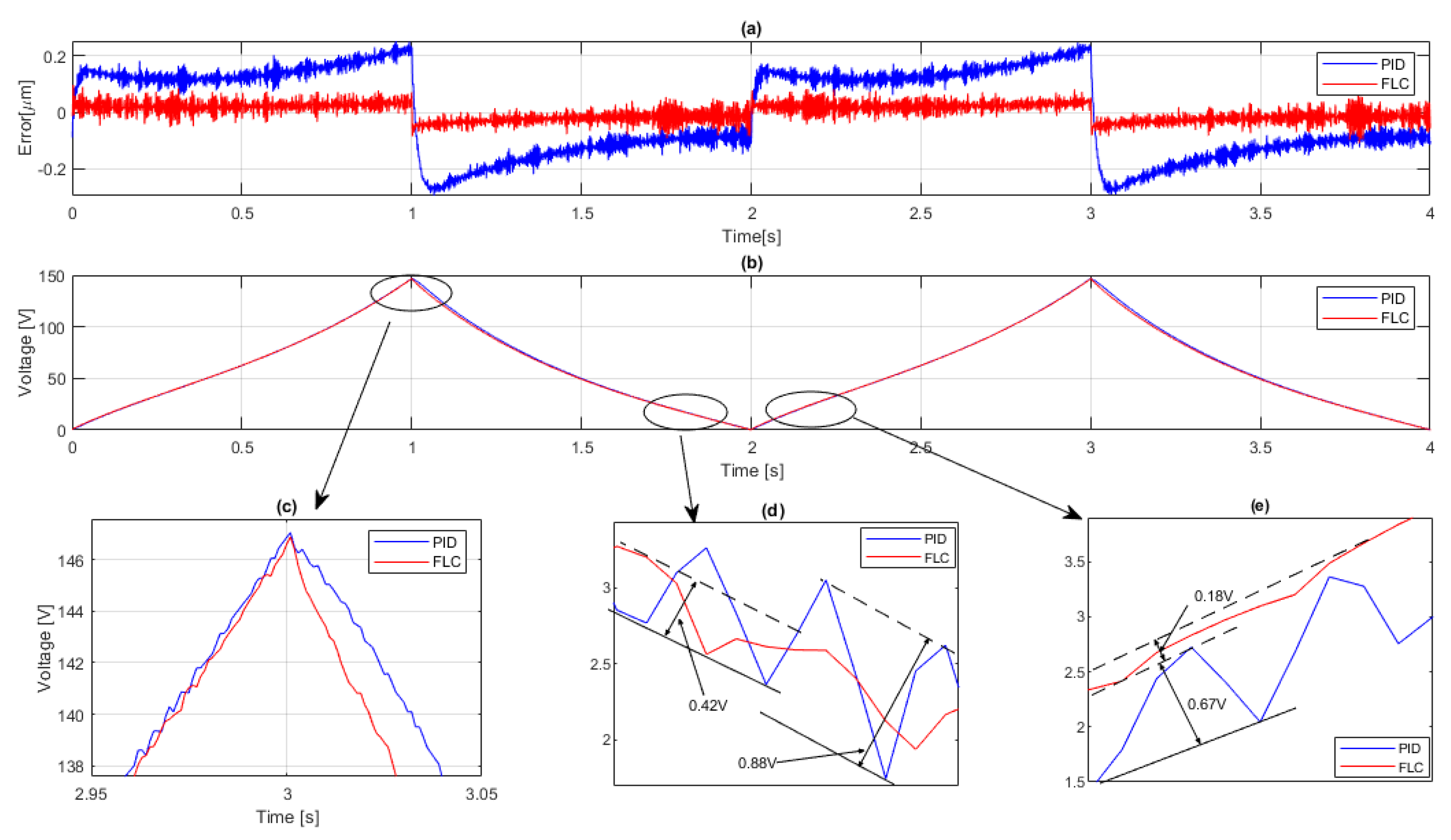
The first contrast was made with a simple PID controller against the FLC. Figure 7a is the error comparison, where it can be seen that the PID has a maximum value that varies between 0.1 and 0.2 $\mathsf{\mu }$m during the rising and descending. However, the relevant feature appears during the peaks where the top ones are at 1 and 3 s, and this yields a severe behaviour where the error flips its sign into the same absolute value, which is expected due to the slope change. Throughout the lower peak, at 2 s, the amplitude of the error was reduced with a smaller value as compared to the top one. On the other hand, the FLC behaves similarly, although the error magnitude was reduced dramatically since its value is below 0.2 $\mathsf{\mu }$m. Additionally, the sign change feature previously explained is still present, but the error was lowered in magnitude during these moments.

As regards the control signal shown in Figure 7b, both of the architectures seemed to behave similarly, but at the top peak, the FLC increased the performance, since the signal is smooth when compared to the conventional PID as Figure 7c shows. In a deep analysis near the lower peak in Figure 7d, it can be seen that, in the descending, the FLC provided a better signal with less noise. Along the analysed area, the FLC reached 0.42 V, whereas the PID resulted in 0.88 V. This means that the FLC supplied a control actuation that has the half of the one provided by the PID. On the other hand, Figure 7e is a reflection of the analysed situation but after the lower peak where the variation is higher since the PID generate 0.67 V and the FLC 0.18 V, which means a difference of around 3.7 times lower for the FLC.

3.5. FLC vs. FLC with HW-FF

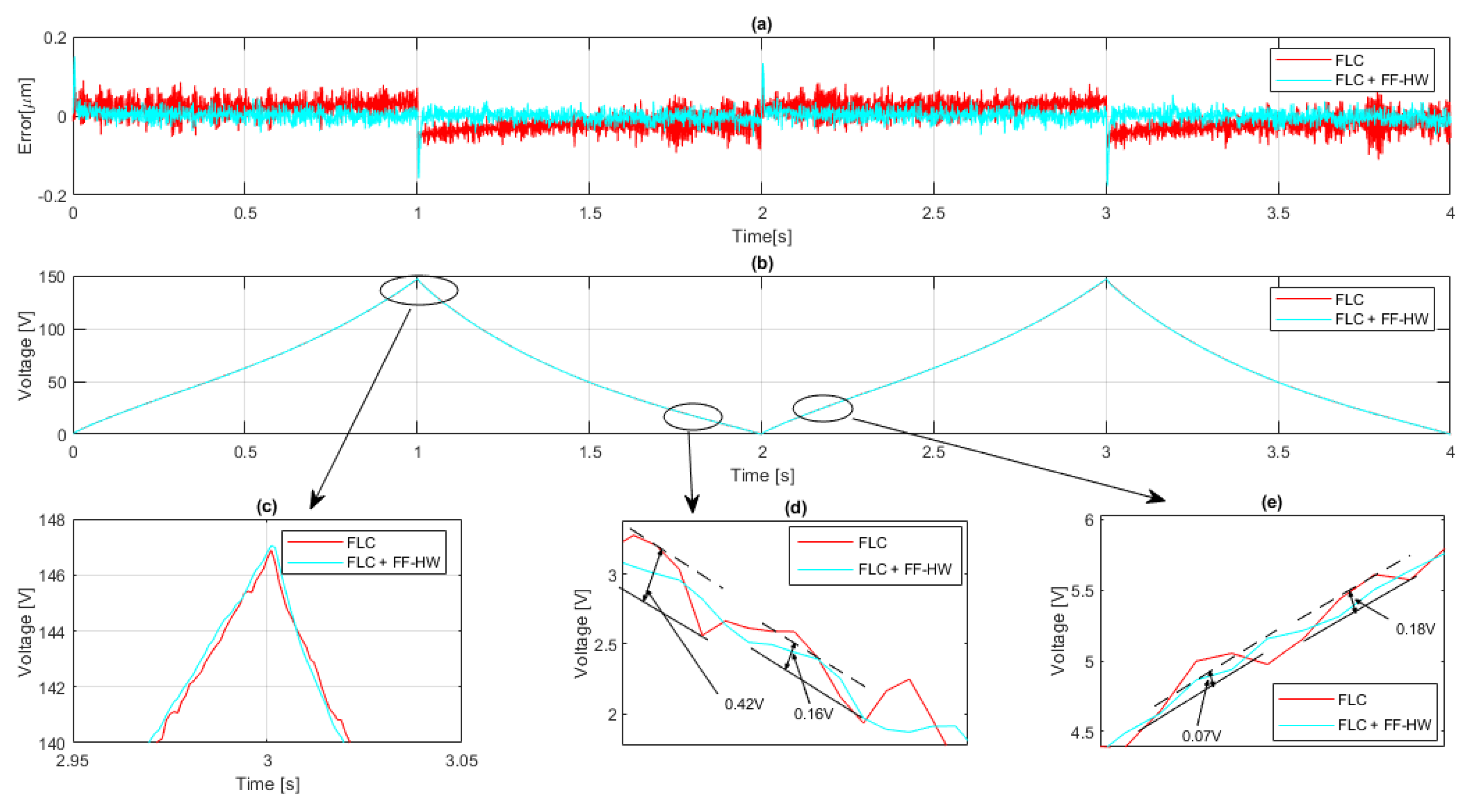
The previous comparison indicated that the FLC performed better than the PID controller and, thus, it was compared with the complex structure with FF since it was expected to increase the performance due to the compensation. Figure 8a shows the error of the two contrasted structures, where the combination of FLC with FF improved the accuracy; although there is a discrepancy during the top peaks, the enhanced framework reduces the error variation, and diminishes the issue at highest levels.

Therefore, the peaks can be analysed in-depth, since the FLC controller still has a change of error sign every one second as previously was evaluated; the FLC-HW could shrink this difference at the cost of increasing the error amplitude at around 0.1 $\mathsf{\mu }$m. However, another critical factor is the speed in which the controller could reduce the error: The FLC has a slow response to reduce the error after a top peak that has a length of about 0.5 s. In opposition, the FLC-HW could counteract with a small perception.

Concerning the control actuation that Figure 8b exposes, the manner is similar to the previous case where both behaved similarly. Figure 8c discloses the mild demeanour described since the signal is acceptable for the complex structure at the top peak. Moreover, the control signal during the lower peak resembles in a similar effort in the FF compensated structure in contrast with the FLC in the feedback alone. For instance, Figure 8d shows a comparison, where the FLC-HW has an amplitude variation of 0.16 V and the FLC developed 0.58 V; this means that the difference is 3.6 times less. Furthermore, this nature is present during the rising at Figure 8e, since the difference is three times less for the FLC-HW, which implies that the control signal had improved in comparison with the FLC and the PID.

3.6. IAE, RMSE, and RRMSE Results

The performance evaluation of all displayed structures was based on the IAE values that were obtained in each experiment which were calculated on a period of 4 s for two triangle cycles. Additionally, other metrics, such as RMSE and relative root-mean-square-error (RRMSE), were calculated to compare the performance in depth. All the values obtained are expressed in the

Table 2. Results obtained of the integral of the absolute error (IAE), root-mean-square error (RMSE) and relative root-mean-square-error (RRMSE).

Structure	IAE	RMSE [$\mathsf{\mu }$m]	RRMSE [%]
PID	0.578	0.153	3.42
FLC	0.111	0.033	0.74
FLC + HW-FF	0.017	0.018	0.38

according to the progress of complexity of each architecture.

Regarding the IAE, the PID, FLC and its combination with HW-FF provided, respectively, values of 0.578, 0.111 and 0.048. Undoubtedly, the progression of the complexity of every structure improved the results which are not only reflected in the error and control figures previously presented but also in the IAE. The difference in value for FLC is 5.2 times less than the PID one, although the discrepancy was still enhanced with the FLC combined with HW where the discrepancy was 2.3 times less compared with the FLC alone.

On the other hand, the RMSE and RRMSE had the same disposition as it was expected. The FLC compared with the PID, showed a considerable difference since the FLC decremented the RMSE to 0.033 $\mathsf{\mu }$m; the RRMSE was reduced to 0.74%. Finally, the complex feedback with FF structure had a higher performance since the RMSE was trimmed to 0.017 and the RRMSE decreased 0.36% respect to the FLC alone.

4. Conclusions

The hysteresis of PEAs represents a problem that can produce a performance reduction when these devices are employed for positioning. In this paper, an analysis of structures was attempted to diminish the error with an acceptable control signal, so as to increase the effectiveness in tracking. All of the results were part of experimental tests with a commercial PEA with its respective driver and measurement device.

First, an HW block was used to map the hysteresis, where it was found that a piece-wise function reflected the non-linearities with acceptable precision and the errors presented could be compensated by adding a feedback controller. Subsequently, the structures proposed to be tested were: PID, FLC and its combination with HW-FF. The first structure was contrasted with the FLC, where the latter presented an enhancement in regards to the error reduction, even at complex situations as peaks of the triangle reference; in terms of the IAE, the improvement resulted in a decline of 5.2 times. The control signal was acceptable, since it mirrored a shrink in the noise, during the delicate situation as in top and lower peak, which is favourable for the PEA life-span.

The use of the FLC with HW-FF not only showed that the error was trimmed to lower values, but also it was compensated during slope changes where previous frameworks suffered difficulties to overcome these variations. As an overall metric, the IAE dwindled 2.3 times less in comparison with the uncompensated feedback. The control signal raised a significant improvement, as the noise was even lower than in the previously tested structure. Performance growth was also viewed in during the peaks, where no saturation or rough changes were observed, which could damage the hardware.

In comparison with recent works that were related to a similar control architecture and device; the results presented in [24] reached an IAE of 0.049, which means that this research could improve 3% of the value; as PEAs are for high-precision, then any enhancement in tracking is completely accepted. Additionally, the authors of [49] provided a similar FLC combined with FF for the PEA with lower displacement range, but the error is higher than the one reached in this research. On the other hand, the study that was done in [46] showed that a neural PID implemented in PEA, could produce a RRMSE of 0.76% for a similar signal.

As future research objectives, there are considerable options and combinations to test with the experimental PEA rig. An increase in the structural complexity yields to an FF compensation with a type-2 FLC, which will need to be evaluated in terms of computational limitations; other feedback structures to be implemented are gain scheduling PID combined with fuzzy logic, also related to the type-1 used in this research. In terms of the FF compensation, an analysis of Hammerstein versus Wiener can be analysed in-depth, such as using artificial neural networks as non-linear blocks at the input or the output.