Nonlinear Operators as Concerns Convex Programming and Applied to Signal Processing

Abstract

Splitting methods have received a lot of attention lately because many nonlinear problems that arise in the areas used, such as signal processing and image restoration, are modeled in mathematics as a nonlinear equation, and this operator is decomposed as the sum of two nonlinear operators. Most investigations about the methods of separation are carried out in the Hilbert spaces. This work develops an iterative scheme in Banach spaces. We prove the convergence theorem of our iterative scheme, applications in common zeros of accretive operators, convexly constrained least square problem, convex minimization problem and signal processing.

1. Introduction

Let $\mathcal{E}$ be a real Banach space. The zero point problem is as follows:

$$\mathrm{find}x\in \mathcal{E}\mathrm{such}\mathrm{that}0\in \mathcal{A}u+\mathcal{B}u,$$

(1)

where $\mathcal{A}:\mathcal{E}\to \mathcal{E}$ is an operator and $\mathcal{B}:\mathcal{E}\to 2^{\mathcal{E}}$ is a set-valued operator. This problem includes, as special cases, convex programming, variational inequalities, split feasibility problem and minimization problem [1,2,3,4,5,6,7]. To be more precise, some concrete problems in machine learning, image processing [4,5], signal processing and linear inverse problem can be modeled mathematically as the form in Equation (1).

Signal processing and numerical optimization are independent scientific fields that have always been mutually influencing each other. Perhaps the most convincing example where the two fields have met is compressed sensing (CS) [2]. Several surveys dedicated to these algorithms and their applications in signal processing have appeared [3,6,7,8].

Fixed point iterations is an important tool for solving various problems and is known in a Banach space $\mathcal{E}$. Let $\mathcal{K}$ be a nonempty closed convex subset of $\mathcal{E}$ and $\mathcal{S}:\mathcal{K}\to \mathcal{K}$ is the operator with at least one fixed point. Then, for $u_1\in \mathcal{K}:$

• The Picard iterative scheme [9] is defined by:

  $$u_{n+1}=\mathcal{S}{u}_n,\forall n\in \mathbb{N}.$$
• The Mann iterative scheme [10] is defined by:

  $$u_{n+1}=(1-{\eta }_n)u_n+{\eta }_n\mathcal{S}{u}_n,\forall n\in \mathbb{N},$$

  where $\left\{{\eta }_n\right\}$ is a sequence in $(0,1).$
• The Ishikawa iterative scheme [11] is defined by:

  $$u_{n+1}=(1-{\eta }_n)u_n+{\eta }_n\mathcal{S}[(1-{\vartheta }_n)u_n+{\vartheta }_n\mathcal{S}{u}_n],\forall n\in \mathbb{N},$$

  where $\left\{{\eta }_n\right\}$ and $\left\{{\vartheta }_n\right\}$ are sequences in $(0,1).$
• The $\mathcal{S}$-iterative scheme [12] is defined by:

  $$u_{n+1}=(1-{\eta }_n)\mathcal{S}{u}_n+{\eta }_n\mathcal{S}[(1-{\vartheta }_n)u_n+{\vartheta }_n\mathcal{S}{u}_n],\forall n\in \mathbb{N},$$

  where $\left\{{\eta }_n\right\}$ and $\left\{{\vartheta }_n\right\}$ are sequences in $(0,1).$

Recently, Sahu et al. [13] and Thakur et al. [14] introduced the following same iterative scheme for nonexpansive mappings in uniformly convex Banach space:

$$\left\{\begin{array}{c}{w}_n=(1-{\xi }_n)u_n+{\xi }_n\mathcal{S}{u}_n,\hfill \\ z_n=(1-{\vartheta }_n)w_n+{\vartheta }_n\mathcal{S}{w}_n,\hfill \\ u_{n+1}=(1-{\eta }_n)\mathcal{S}{w}_n+{\eta }_n\mathcal{S}{z}_n,\forall n\in \mathbb{N},\hfill \end{array}\right.$$

where $\left\{{\eta }_n\right\},\left\{{\vartheta }_n\right\}$ and $\left\{{\xi }_n\right\}$ are sequences in $(0,1)$. The authors proved that this scheme converges to a fixed point of contraction mapping, faster than all known iterative schemes. In addition, the authors provided an example to support their claim.

In this paper, we first develop an iterative scheme for calculating common solutions and using our results to solve the problem in Equation (1). Secondly, we find common solutions of convexly constrained least square problems, convex minimization problems and applied to signal processing.

2. Preliminaries

Let $\mathcal{E}$ be a real Banach space with norm $\parallel ·\parallel$ and ${\mathcal{E}}^{\ast }$ be its dual. The value of $f\in {\mathcal{E}}^{\ast }$ at $u\in \mathcal{E}$ ia denoted by $\langle u,f\rangle .$ A Banach space $\mathcal{E}$ is called strictly convex if $\frac{\parallel u+v\parallel }{2}<1,$ for all $u,v\in \mathcal{E}$ with $\parallel u\parallel =\parallel v\parallel =1.$ It is called uniformly convex if ${lim}_{n\to \infty }\parallel u_n-v_n\parallel =0$ for any two sequences $\left\{u_n\right\},\left\{v_n\right\}$ in $\mathcal{E}$ such that $\parallel u\parallel =\parallel v\parallel =1$ and ${lim}_{n\to \infty }\frac{\parallel u+v\parallel }{2}=1.$

The (normalized) duality mapping $\mathcal{J}$ from $\mathcal{E}$ into the family of nonempty (by Hahn Banach theorem) weak-star compact subsets of its dual $\mathcal{E}$ is defined by

$$\mathcal{J}\left(u\right)=\{f\in {\mathcal{E}}^{\ast }:\langle u,f\rangle =\parallel u{\parallel }^2=\parallel f{\parallel }^2\}$$

for each $u\in \mathcal{E},$ where $\langle ·,·\rangle$ denotes the generalized duality pairing.

For an operator $\mathcal{A}:\mathcal{E}\to 2^{\mathcal{E}},$ we denote its domain, range and graph as follows:

$$\begin{array}{cc}\hfill \mathcal{D}\left(\mathcal{A}\right)& =\{u\in \mathcal{E}:\mathcal{A}u\ne \varnothing \}\hfill \\ \hfill \mathcal{R}\left(\mathcal{A}\right)& =\cup \{\mathcal{A}p:p\in \mathcal{D}(\mathcal{A}\left)\right\},\hfill \end{array}$$

and

$$\mathcal{G}\left(\mathcal{A}\right)=\left\{\right(u,v)\in \mathcal{E}\times \mathcal{E}:u\in \mathcal{D}(\mathcal{A}),v\in \mathcal{A}u\},$$

respectively. The inverse ${\mathcal{A}}^{-1}$ of $\mathcal{A}$ is defined by $u\in {\mathcal{A}}^{-1}v,$ if and only if $v\in \mathcal{A}u.$ If $\forall u_i\in \mathcal{D}\left(\mathcal{A}\right)$ and $v_i\in \mathcal{A}{u}_i(i=1,2),$ and there is $j\in \mathcal{J}(u_1-u_2)$ such that $\langle v_1-v_2,j\rangle \ge 0,$ then $\mathcal{A}$ is called accretive.

An accretive operator $\mathcal{A}$ in a Banach space $\mathcal{E}$ is said to satisfy the range condition if $\overline{\mathcal{D}\left(\mathcal{A}\right)}\subset \mathcal{R}(I+\mu \mathcal{A})$ for all $\mu >0,$ where $\overline{\mathcal{D}\left(\mathcal{A}\right)}$ denotes the closure of the domain of $\mathcal{A}.$ We know that for an accretive operator $\mathcal{A}$ which satisfies the range condition, ${\mathcal{A}}^{-1}0=\mathcal{F}ix\left({\mathcal{J}}_{\mu }^{\mathcal{A}}\right)$ for all $\mu >0.$

A point $u\in \mathcal{K}$ is a fixed point of $\mathcal{S}$ provided $\mathcal{S}u=u.$ Denote by $\mathcal{F}ix\left(\mathcal{S}\right)$ the set of fixed points of $\mathcal{S}$, i.e., $\mathcal{F}ix\left(\mathcal{S}\right)=\{u\in \mathcal{K}:\mathcal{S}u=u\}.$

• The mapping $\mathcal{S}$ is called $\mathcal{L}–$Lipschitz, $\mathcal{L}>0$, if

  $$\parallel \mathcal{S}u-\mathcal{S}v\parallel \le \mathcal{L}\parallel u-v\parallel ,\forall u,v\in \mathcal{K}.$$
• The mapping $\mathcal{S}$ is called nonexpansive if

  $$\parallel \mathcal{S}u-\mathcal{S}v\parallel \le \parallel u-v\parallel ,\forall u,v\in \mathcal{K}.$$
• The mapping $\mathcal{S}$ is called quasi-nonexpansive if $\mathcal{F}ix\left(\mathcal{S}\right)\ne \varnothing$ and

  $$\parallel \mathcal{S}u-v\parallel \le \parallel u-v\parallel ,\forall u\in \mathcal{K},v\in \mathcal{F}ix\left(\mathcal{S}\right).$$

In this case, $\mathcal{H}$ is a real Hilbert space. If $\mathcal{A}:\mathcal{E}\to 2^{\mathcal{E}}$ is an $m–$accretive operator (see [15,16,17]), then $\mathcal{A}$ is called maximal accretive operator [18], and for all $\mu >0$, $\mathcal{R}(I+\mu \mathcal{A})=\mathcal{H}$ if and only if $\mathcal{A}$ is called maximal monotone [19]. Denote by $\mathrm{dom}\left(h\right)$ the domain of a function $h:\mathcal{H}\to (-\infty ,\infty ],\mathrm{i}.\mathrm{e}.,$

$$\mathrm{dom}\left(h\right)=\{u\in \mathcal{H}:h(u)<\infty \}.$$

The subdifferential of $h\in {\mathsf{\Gamma }}_0\left(\mathcal{H}\right)$ at $u\in \mathcal{H}$ is the set

$$\partial h\left(u\right)=\{z\in \mathcal{H}:h(u)\le h(v)+\langle z,u-v\rangle ,\forall v\in \mathcal{H}\},$$

where ${\mathsf{\Gamma }}_0\left(\mathcal{H}\right)$ denotes the class of all $l.s.c.$ functions from $\mathcal{H}$ to $(-\infty ,\infty ]$ with nonempty domains.

Lemma 1

([20]). Let $h\in {\mathsf{\Gamma }}_0\left(\mathcal{H}\right).$ Then, $\partial h$ is maximal monotone.

We denote by $B_{\lambda }\left[v\right]$ the closed ball with the center at v and radius $\lambda :$

$$B_{\lambda }\left[v\right]=\{u\in \mathcal{E}:\parallel v-u\parallel \le \lambda \}.$$

Lemma 2

([21]). Let $\mathcal{E}$ be a Banach space, and $p>1$ and $R>0$ be two fixed numbers. Then, $\mathcal{E}$ is uniformly convex if and only if there exists a continuous, strictly increasing, and convex function $\phi :[0,\infty )\to [0,\infty )$ with $\phi \left(0\right)=0$ such that

$${\parallel \alpha u+(1-\alpha )v\parallel }^p\le {\parallel u\parallel }^p+{(1-\alpha )\parallel v\parallel }^p-\alpha (1-\alpha )\phi (\parallel u-v\parallel ),$$

for all $u,v\in B_R\left[0\right]$ and $\alpha \in [0,1].$

Definition 1

([22]). A vector space $\mathcal{H}$ is said to satisfy Opial’s condition, if for each sequence $\left\{u_n\right\}$ in $\mathcal{H}$ which converges weakly to point $u\in \mathcal{H},$

$$\underset{n\to \infty }{lim\; inf}\parallel u_n-u\parallel <\underset{n\to \infty }{lim\; inf}\parallel u_n-v\parallel ,v\in \mathcal{H},v\ne u.$$

Lemma 3

([23]). Let $\mathcal{K}$ be a nonempty subset of a Banach space $\mathcal{E}$, let $\mathcal{S}:\mathcal{K}\to \mathcal{E}$ be a uniformly continuous mapping, and let $\left\{u_n\right\}\subset \mathcal{K}$ an approximating fixed point sequence of $\mathcal{S}.$ Then, $\left\{v_n\right\}$ is an approximating fixed point sequence of $\mathcal{S}$ whenever $\left\{v_n\right\}$ is in $\mathcal{K}$ such that ${lim}_{n\to \infty }\parallel u_n-v_n\parallel =0.$

Lemma 4

([16]). Let $\mathcal{K}$ be a nonempty closed convex subset of a uniformly convex Banach space $\mathcal{E}$. If $\mathcal{S}:\mathcal{K}\to \mathcal{E}$ is a nonexpansive mapping, then $I-\mathcal{S}$ has the demiclosed property with respect to $0.$

A subset $\mathcal{K}$ of Banach space $\mathcal{E}$ is called a retract of $\mathcal{E}$ if there is a continuous mapping $\mathcal{Q}$ from $\mathcal{E}$ onto $\mathcal{K}$ such that $\mathcal{Q}u=u$ for all $u\in \mathcal{K}.$ We call such $\mathcal{Q}$ a retraction of $\mathcal{E}$ onto $\mathcal{K}.$ It follows that, if a mapping $\mathcal{Q}$ is a retraction, then $\mathcal{Q}v=v$ for all v in the range of $\mathcal{Q}.$ A retraction $\mathcal{Q}$ is called a sunny if $\mathcal{Q}(\mathcal{Q}u+\lambda (u-\mathcal{Q}u\left)\right)=\mathcal{Q}u$ for all $u\in \mathcal{E}$ and $\lambda \ge 0.$ If a sunny retraction $\mathcal{Q}$ is also nonexpansive, then $\mathcal{K}$ is called a sunny nonexpansive retract of $\mathcal{E}$ [24].

Let $\mathcal{E}$ be a strictly convex reflexive Banach space and $\mathcal{K}$ be a nonempty closed convex subset of $\mathcal{E}.$ Denote by ${\mathcal{P}}_{\mathcal{K}}$ the (metric) projection from $\mathcal{E}$ onto $\mathcal{K}$, namely, for $u\in \mathcal{E},{\mathcal{P}}_{\mathcal{K}}\left(u\right)$ is the unique point in $\mathcal{K}$ with the property

$$inf\{\parallel u-v\parallel :v\in \mathcal{K}\}=\parallel u-{\mathcal{P}}_{\mathcal{K}}\left(u\right)\parallel .$$

Let an inner product $\langle ·,·\rangle$ and the induced norm $\parallel ·\parallel$ are specified with a real Hilbert space $\mathcal{H}$. Let $\mathcal{K}$ is a nonempty subset of $\mathcal{H}$, we have the nearest point projection ${\mathcal{P}}_{\mathcal{K}}:\mathcal{H}\to \mathcal{K}$ is the unique sunny nonexpansive retraction of $\mathcal{H}$ onto $\mathcal{K}.$ It is also known that ${\mathcal{P}}_{\mathcal{K}}\left(u\right)\in \mathcal{K}$ and

$$\langle u-{\mathcal{P}}_{\mathcal{K}}\left(u\right),{\mathcal{P}}_{\mathcal{K}}\left(u\right)-v\rangle \ge 0,\forall u\in \mathcal{H},v\in \mathcal{K}.$$

3. Main Results

Let $\mathcal{K}$ be a nonempty closed convex subset of a Banach space $\mathcal{E}$ with ${\mathcal{Q}}_{\mathcal{K}}$ as a sunny nonexpansive retraction. We denote by $\mathsf{\Psi }:=\mathcal{F}ix\left(\mathcal{S}\right)\cap \mathcal{F}ix\left(\mathcal{T}\right)$.

Lemma 5.

Let $\mathcal{K}$ be a nonempty closed convex subset of a Banach space $\mathcal{E}$ with ${\mathcal{Q}}_{\mathcal{K}}$ as the sunny nonexpansive retraction, let $\mathcal{S},\mathcal{T}:\mathcal{K}\to \mathcal{E}$ be quasi-nonexpansive mappings which $\mathsf{\Psi }\ne \varnothing ,$ and let $\left\{{\eta }_n\right\},\left\{{\vartheta }_n\right\}$ and $\left\{{\xi }_n\right\}$ be sequences in $(0,1)$ for all $n\in \mathbb{N}.$ Let $\left\{u_n\right\}$ be defined by Algorithm 1. Then, for each $\overline{u}\in \mathsf{\Psi },{lim}_{n\to \infty }\parallel u_n-\overline{u}\parallel$ exists and

$$\parallel w_n-\overline{u}\left|\right|\le \parallel u_n-\overline{u}\parallel ,and\parallel z_n-\overline{u}\parallel \le \parallel u_n-\overline{u}\parallel ,\forall n\in \mathbb{N}.$$

(2)

Algorithm 1: Three-step sunny nonexpansive retraction

Proof. 

Let $\overline{u}\in \mathsf{\Psi }.$ Then, we have

$$\begin{array}{cc}\hfill \parallel w_n-\overline{u}\parallel & =\parallel {\mathcal{Q}}_{\mathcal{K}}[(1-{\xi }_n)u_n+{\xi }_n\mathcal{S}{u}_n]-\overline{u}\parallel \hfill \\ & \le \parallel (1-{\xi }_n)(u_n-\overline{u})+{\xi }_n(\mathcal{S}{u}_n-\overline{u})\parallel \hfill \\ & \le (1-{\xi }_n)\parallel u_n-\overline{u}\parallel +{\xi }_n\parallel \mathcal{S}{u}_n-\overline{u}\parallel \hfill \\ & \le (1-{\xi }_n)\parallel u_n-\overline{u}\parallel +{\xi }_n\parallel u_n-\overline{u}\parallel \hfill \\ & =\parallel u_n-\overline{u}\parallel ,\hfill \end{array}$$

(3)

$$\begin{array}{cc}\hfill \parallel z_n-\overline{u}\parallel & =\parallel {\mathcal{Q}}_{\mathcal{K}}[(1-{\vartheta }_n)w_n+{\vartheta }_n\mathcal{T}{w}_n]-\overline{u}\parallel \hfill \\ & \le \parallel (1-{\vartheta }_n)(w_n-\overline{u})+{\vartheta }_n(\mathcal{T}{w}_n-\overline{u})\parallel \hfill \\ & \le (1-{\vartheta }_n)\parallel w_n-\overline{u}\parallel +{\vartheta }_n\parallel \mathcal{T}{w}_n-\overline{u}\parallel \hfill \\ & \le (1-{\vartheta }_n)\parallel w_n-\overline{u}\parallel +{\vartheta }_n\parallel w_n-\overline{u}\parallel \hfill \\ & =\parallel w_n-\overline{u}\parallel \hfill \\ & \le \parallel u_n-\overline{u}\parallel ,\hfill \end{array}$$

(4)

and

$$\begin{array}{cc}\hfill \parallel u_{n+1}-\overline{u}\parallel & =\parallel {\mathcal{Q}}_{\mathcal{K}}[(1-{\eta }_n)\mathcal{S}{w}_n+{\eta }_n\mathcal{T}{z}_n]-\overline{u}\parallel \hfill \\ & \le \parallel (1-{\eta }_n)(\mathcal{S}{w}_n-\overline{u})+{\eta }_n(\mathcal{T}{z}_n-\overline{u})\parallel \hfill \\ & \le (1-{\eta }_n)\parallel \mathcal{S}{w}_n-\overline{u}\parallel +{\eta }_n\parallel \mathcal{T}{z}_n-\overline{u}\parallel \hfill \\ & \le (1-{\eta }_n)\parallel w_n-\overline{u}\parallel +{\eta }_n\parallel z_n-\overline{u}\parallel \hfill \\ & \le (1-{\eta }_n)\parallel u_n-\overline{u}\parallel +{\eta }_n\parallel u_n-\overline{u}\parallel \hfill \\ & =\parallel u_n-\overline{u}\parallel .\hfill \end{array}$$

(5)

Therefore,

$$\parallel u_{n+1}-\overline{u}\parallel \le \parallel u_n-\overline{u}\parallel \le \cdots \le \parallel u_1-\overline{u}\parallel ,\forall n\in \mathbb{N}.$$

(6)

Since $\{\parallel u_n-\overline{u}\parallel \}$ is monotonically decreasing, we have that the sequence $\{\parallel u_n-\overline{u}\parallel \}$ is convergent. □

From Lemma 5, we have results:

Theorem 1.

Let $\mathcal{K}$ be a nonempty closed convex subset of a Banach space $\mathcal{E}$ with ${\mathcal{Q}}_{\mathcal{K}}$ as the sunny nonexpansive retraction, let $\mathcal{S},\mathcal{T}:\mathcal{K}\to \mathcal{E}$ be quasi-nonexpansive mappings with $\mathsf{\Psi }\ne \varnothing ,$ and let $\left\{{\eta }_n\right\},\left\{{\vartheta }_n\right\}$ and $\left\{{\xi }_n\right\}$ be sequences of real numbers, for which $0<c_1\le {\eta }_n\le {\widehat{c}}_1<1,0<c_2\le {\vartheta }_n\le {\widehat{c}}_2<1,0<c_3\le {\xi }_n\le {\widehat{c}}_3<1$ for all $n\in \mathbb{N}.$ Let $u_1\in \mathcal{K},{\mathcal{P}}_{\mathsf{\Psi }}\left(u_1\right)=u_{\ast }$ and $\left\{u_n\right\}$ is defined by Algorithm 1. Then, we have the following:

(i) 

$\left\{u_n\right\}$ is in a closed convex bounded set $B_{\lambda }\left[u_{\ast }\right]\cap \mathcal{K},$ where λ is a constant in $(0,\infty )$ such that $\parallel u_1-u_{\ast }\parallel \le \lambda .$

(ii) 

If $\mathcal{S}$ is uniformly continuous, then ${lim}_{n\to \infty }\parallel u_n-\mathcal{S}{u}_n\parallel =0$ and ${lim}_{n\to \infty }\parallel u_n-\mathcal{T}{u}_n\parallel =0.$

(iii) 

If $\mathcal{E}$ fulfills the Opial’s condition and $I-\mathcal{S}$ and $I-\mathcal{T}$ are demiclosed at $0,$ then $\left\{u_n\right\}$ converges weakly to an element of $\mathsf{\Psi }\cap B_{\lambda }\left[u_{\ast }\right].$

Proof. 

$\left(\mathrm{i}\right)$ Since $u_{\ast }\in \mathsf{\Psi },$ from Equation (6), we obtain

$$\parallel u_{n+1}-u_{\ast }\parallel \le \parallel u_n-u_{\ast }\parallel \le \cdots \le \parallel u_1-u_{\ast }\parallel \le \lambda ,\forall n\in \mathbb{N}.$$

(7)

Therefore, $\left\{u_n\right\}$ is in the closed convex bounded set $B_{\lambda }\left[u_{\ast }\right]\cap \mathcal{K}.$

$\left(\mathrm{ii}\right)$ Suppose that $\mathcal{S}$ is uniformly continuous. Using Lemma 5, we get that $\left\{u_n\right\},\left\{z_n\right\}$ and $\left\{w_n\right\}$ are in $B_{\lambda }\left[u_{\ast }\right]\cap \mathcal{K},$ and hence, from Equation (2), we obtain

$$\parallel \mathcal{T}{w}_n-u_{\ast }\parallel \le \lambda ,\parallel \mathcal{S}{w}_n-u_{\ast }\parallel \le \lambda \mathrm{and}\parallel \mathcal{S}{u}_n-u_{\ast }\parallel \le \lambda ,\forall n\in \mathbb{N}.$$

Using Lemma 2 for $p=2$ and $R=\lambda ,$ from Equation (5), we obtain

$$\begin{array}{cc}\hfill \parallel u_{n+1}-u_{\ast }{\parallel }^2& \le \parallel (1-{\eta }_n)(\mathcal{S}{w}_n-u_{\ast })+{\eta }_n(\mathcal{T}{z}_n-u_{\ast }){\parallel }^2\hfill \\ & \le (1-{\eta }_n)\parallel \mathcal{S}{w}_n-u_{\ast }{\parallel }^2+{\eta }_n\parallel \mathcal{T}{z}_n-u_{\ast }{\parallel }^2\hfill \\ & -{\eta }_n(1-{\eta }_n)\phi (\parallel \mathcal{S}{w}_n-\mathcal{T}{z}_n\parallel )\hfill \\ & \le (1-{\eta }_n)\parallel w_n-u_{\ast }{\parallel }^2+{\eta }_n\parallel z_n-u_{\ast }{\parallel }^2\hfill \\ & -{\eta }_n(1-{\eta }_n)\phi (\parallel \mathcal{S}{w}_n-\mathcal{T}{z}_n\parallel )\hfill \\ & \le (1-{\eta }_n)\parallel u_n-u_{\ast }{\parallel }^2+{\eta }_n\parallel u_n-u_{\ast }{\parallel }^2\hfill \\ & -{\eta }_n(1-{\eta }_n)\phi (\parallel \mathcal{S}{w}_n-\mathcal{T}{z}_n\parallel )\hfill \\ & =\parallel u_n-u_{\ast }{\parallel }^2-{\eta }_n(1-{\eta }_n)\phi (\parallel \mathcal{S}{w}_n-\mathcal{T}{z}_n\parallel ),\hfill \end{array}$$

(8)

which implies that

$${\eta }_n(1-{\eta }_n)\phi (\parallel \mathcal{S}{w}_n-\mathcal{T}{z}_n\parallel )=\parallel u_n-u_{\ast }\parallel -\parallel u_{n+1}-u_{\ast }{\parallel }^2.$$

(9)

Note that: $c_1(1-{\widehat{c}}_1)\le {\eta }_n(1-{\eta }_n).$ Thus,

$$c_1(1-{\widehat{c}}_1)\sum _{i=1}^n\phi (\parallel \mathcal{S}{w}_i-\mathcal{T}{z}_i\parallel )=\parallel u_1-u_{\ast }\parallel -\parallel u_{n+1}-u_{\ast }{\parallel }^2,\forall n\in \mathbb{N}.$$

(10)

In the same way, we obtain

$$c_1(1-{\widehat{c}}_1)\sum _{n=1}^{\infty }\phi (\parallel \mathcal{S}{w}_n-\mathcal{T}{z}_n\parallel )\le \parallel u_1-u_{\ast }\parallel <\infty .$$

(11)

Therefore, we have ${lim}_{n\to \infty }\parallel \mathcal{S}{w}_n-\mathcal{T}{z}_n\parallel =0.$ From the relations in Algorithm 1, we obtain

$$\begin{array}{cc}\hfill \parallel w_n-u_{\ast }{\parallel }^2& \le (1-{\xi }_n)\parallel u_n-u_{\ast }{\parallel }^2+{\xi }_n\parallel \mathcal{S}{u}_n-u_{\ast }{\parallel }^2\hfill \\ & -{\xi }_n(1-{\xi }_n)\phi (\parallel u_n-\mathcal{S}{u}_n\parallel )\hfill \\ & \le (1-{\xi }_n)\parallel u_n-u_{\ast }{\parallel }^2+{\xi }_n\parallel u_n-u_{\ast }{\parallel }^2\hfill \\ & -{\xi }_n(1-{\xi }_n)\phi (\parallel u_n-\mathcal{S}{u}_n\parallel )\hfill \\ & =\parallel u_n-u_{\ast }{\parallel }^2-{\xi }_n(1-{\xi }_n)\phi (\parallel u_n-\mathcal{S}{u}_n\parallel )\hfill \end{array}$$

(12)

and

$$\begin{array}{cc}\hfill \parallel z_n-u_{\ast }{\parallel }^2& \le \parallel (1-{\vartheta }_n)(w_n-u_{\ast })+{\vartheta }_n(\mathcal{T}{w}_n-u_{\ast }){\parallel }^2\hfill \\ & \le (1-{\vartheta }_n)\parallel w_n-u_{\ast }{\parallel }^2+{\vartheta }_n\parallel \mathcal{T}{w}_n-u_{\ast }{\parallel }^2\hfill \\ & -{\vartheta }_n(1-{\vartheta }_n)\phi (\parallel w_n-\mathcal{T}{w}_n\parallel )\hfill \\ & \le (1-{\vartheta }_n)\parallel w_n-u_{\ast }{\parallel }^2+{\vartheta }_n\parallel w_n-u_{\ast }{\parallel }^2\hfill \\ & =\parallel w_n-u_{\ast }{\parallel }^2-{\vartheta }_n(1-{\vartheta }_n)\phi (\parallel w_n-\mathcal{T}{w}_n\parallel )\hfill \\ & \le \parallel u_n-u_{\ast }{\parallel }^2-{\vartheta }_n(1-{\vartheta }_n)\phi (\parallel w_n-\mathcal{T}{w}_n\parallel ).\hfill \end{array}$$

(13)

From Equations (8), (13) and (12), we obtain

$$\begin{array}{cc}\hfill \parallel u_{n+1}-u_{\ast }{\parallel }^2& \le \parallel (1-{\eta }_n)(\mathcal{S}{w}_n-u_{\ast })+{\eta }_n(\mathcal{T}{z}_n-u_{\ast }){\parallel }^2\hfill \\ & \le (1-{\eta }_n)\parallel \mathcal{S}{w}_n-u_{\ast }{\parallel }^2+{\eta }_n\parallel \mathcal{T}{z}_n-u_{\ast }{\parallel }^2\hfill \\ & -{\eta }_n(1-{\eta }_n)\phi (\parallel \mathcal{S}{w}_n-\mathcal{T}{z}_n\parallel )\hfill \\ & \le (1-{\eta }_n)\parallel w_n-u_{\ast }{\parallel }^2+{\eta }_n\parallel z_n-u_{\ast }{\parallel }^2\hfill \\ & -{\eta }_n(1-{\eta }_n)\phi (\parallel \mathcal{S}{w}_n-\mathcal{T}{z}_n\parallel )\hfill \\ & \le (1-{\eta }_n)[\parallel u_n-u_{\ast }{\parallel }^2-{\xi }_n(1-{\xi }_n)\phi (\parallel u_n-\mathcal{S}{u}_n\parallel \left)\right]\hfill \\ & +{\eta }_n[\parallel u_n-u_{\ast }{\parallel }^2-{\vartheta }_n(1-{\vartheta }_n)\phi (\parallel w_n-\mathcal{T}{w}_n\parallel \left)\right]\hfill \\ & -{\eta }_n(1-{\eta }_n)\phi (\parallel \mathcal{S}{w}_n-\mathcal{T}{z}_n\parallel )\hfill \\ & =\parallel u_n-u_{\ast }{\parallel }^2-(1-{\eta }_n){\xi }_n(1-{\xi }_n)\phi (\parallel u_n-\mathcal{S}{u}_n\parallel )\hfill \\ & -{\eta }_n{\vartheta }_n(1-{\vartheta }_n)\phi (\parallel w_n-\mathcal{T}{w}_n\parallel )\hfill \\ & -{\eta }_n(1-{\eta }_n)\phi (\parallel \mathcal{S}{w}_n-\mathcal{T}{z}_n\parallel ).\hfill \end{array}$$

(14)

Note that: $(1-{\widehat{c}}_1)c_3(1-{\widehat{c}}_3)\le (1-{\eta }_n){\xi }_n(1-{\xi }_n)$ and $c_1{c}_2(1-{\widehat{c}}_2)\le {\eta }_n{\vartheta }_n(1-{\vartheta }_n).$ Thus,

$$(1-{\widehat{c}}_1)c_3(1-{\widehat{c}}_3)\sum _{i=1}^n\phi (\parallel u_i-\mathcal{S}{u}_i\parallel )\le \parallel u_1-u_{\ast }{\parallel }^2-{\parallel u_{n+1}-u_{\ast }\parallel }^2,\forall n\in \mathbb{N}.$$

It follows that ${lim}_{n\to \infty }\parallel u_n-\mathcal{S}{u}_n\left|\right|=0.$ Note that:

$$\begin{array}{cc}\hfill \parallel w_n-u_n\parallel & =\parallel {\mathcal{Q}}_{\mathcal{K}}[(1-{\xi }_n)u_n+{\xi }_n\mathcal{S}{u}_n]-{\mathcal{Q}}_{\mathcal{K}}\left[u_n\right]\parallel \hfill \\ & \le \parallel \mathcal{S}{u}_n-u_n\parallel \to 0\mathrm{as}n\to \infty .\hfill \end{array}$$

Since $\mathcal{S}$ is uniformly continuous, it follows from Lemma 3 that ${lim}_{n\to \infty }\parallel w_n-\mathcal{S}{w}_n\parallel =0.$ Thus, from ${lim}_{n\to \infty }\parallel \mathcal{S}{w}_n-\mathcal{T}{z}_n\parallel =0,$ we obtain ${lim}_{n\to \infty }\parallel u_n-\mathcal{T}{u}_n\parallel =0.$

$\left(\mathrm{iii}\right)$ By assumption, $\mathcal{E}$ satisfies the Opial’s condition. Let $w^{\ast }\in \mathsf{\Psi }$ such that $w^{\ast }\in B_{\lambda }\left[u_{\ast }\right]\cap \mathcal{K}.$ From Lemma 5, we have ${lim}_{n\to \infty }\parallel u_n-w^{\ast }\parallel$ exists. Suppose there are two subsequences $\left\{u_{n_q}\right\}$ and $\left\{u_{m_l}\right\}$ which converge to two distinct points $u^{\ast }$ and $v^{\ast }$ in $B_{\lambda }\left[u_{\ast }\right]\cap \mathcal{K},$ respectively. Then, since both $I-\mathcal{S}$ and $I-\mathcal{T}$ have the demiclosed property at $0,$ we have $\mathcal{S}{u}^{\ast }=\mathcal{T}{u}^{\ast }=u^{\ast }$ and $\mathcal{S}{v}^{\ast }=\mathcal{T}{v}^{\ast }=v^{\ast }.$ Moreover, using the Opial’s condition:

$$\underset{n\to \infty }{lim}\parallel u_n-u^{\ast }\parallel =\underset{q\to \infty }{lim}\parallel u_{n_q}-u^{\ast }\parallel <\underset{l\to \infty }{lim}\parallel u_{m_l}-v^{\ast }\parallel =\underset{n\to \infty }{lim}\parallel u_n-v^{\ast }\parallel .$$

Similarly, we obtain

$$\underset{n\to \infty }{lim}\parallel u_n-v^{\ast }\parallel <\underset{n\to \infty }{lim}\parallel u_n-u^{\ast }\parallel ,$$

which is a contradiction. Therefore, $u^{\ast }=v^{\ast }.$ Hence, the sequence $\left\{u_n\right\}$ converges weakly to an element of $\mathsf{\Psi }\cap B_{\lambda }\left[u_{\ast }\right]\cap \mathcal{K}.$ □

Theorem 2.

Let $\mathcal{K}$ be a nonempty closed convex subset of a Banach space $\mathcal{E}$ with ${\mathcal{Q}}_{\mathcal{K}}$ as the sunny nonexpansive retraction, let $\mathcal{S},\mathcal{T}:\mathcal{K}\to \mathcal{E}$ be nonexpansive mappings with $\mathsf{\Psi }\ne \varnothing ,$ and let $\left\{{\eta }_n\right\},\left\{{\vartheta }_n\right\}$ and $\left\{{\xi }_n\right\}$ be sequences of real numbers, for which $0<c_1\le {\eta }_n\le {\widehat{c}}_1<1,0<c_2\le {\vartheta }_n\le {\widehat{c}}_2<1,0<c_3\le {\xi }_n\le {\widehat{c}}_3<1$ for all $n\in \mathbb{N}.$ Let $u_1\in \mathcal{K},{\mathcal{P}}_{\mathsf{\Psi }}\left(u_1\right)=u_{\ast }$ and $\left\{u_n\right\}$ is defined by Algorithm 1. Then, we have the following:

(i) 

$\left\{u_n\right\}$ is in a closed convex bounded set $B_{\lambda }\left[u_{\ast }\right]\cap \mathcal{K},$ where λ is a constant in $(0,\infty )$ such that $\parallel u_1-u_{\ast }\parallel \le \lambda .$

(ii) 

${lim}_{n\to \infty }\parallel u_n-\mathcal{S}{u}_n\parallel =0$ and ${lim}_{n\to \infty }\parallel u_n-\mathcal{T}{u}_n\parallel =0.$

(iii) 

If $\mathcal{E}$ fulfills the Opial’s condition, then $\left\{u_n\right\}$ converges weakly to an element of $\mathsf{\Psi }\cap B_{\lambda }\left[u_{\ast }\right].$

Proof. 

It follows from Theorem 1. □

Corollary 1.

Let $\mathcal{K}$ be a nonempty closed convex subset of a real Hilbert space $\mathcal{H},$ let $\mathcal{S},\mathcal{T}:\mathcal{K}\to \mathcal{E}$ be nonexpansive mappings with $\mathsf{\Psi }\ne \varnothing ,$ and let $\left\{{\eta }_n\right\},\left\{{\vartheta }_n\right\}$ and $\left\{{\xi }_n\right\}$ be sequences of real numbers, for which $0<c_1\le {\eta }_n\le {\widehat{c}}_1<1,0<c_2\le {\vartheta }_n\le {\widehat{c}}_2<1,0<c_3\le {\xi }_n\le {\widehat{c}}_3<1$ for all $n\in \mathbb{N}.$ Let $\left\{u_n\right\}$ be defined by

$$\left\{\begin{array}{c}{w}_n=(1-{\xi }_n)u_n+{\xi }_n\mathcal{S}{u}_n,\hfill \\ z_n=(1-{\vartheta }_n)w_n+{\vartheta }_n\mathcal{T}{w}_n,\hfill \\ u_{n+1}=(1-{\eta }_n)\mathcal{S}{w}_n+{\eta }_n\mathcal{T}{z}_n,\forall n\in \mathbb{N}.\hfill \end{array}\right.$$

(15)

Then, $\left\{u_n\right\}$ converges weakly to an element of $\mathsf{\Psi }.$

Proof. 

It follows from Theorem 1. □

4. Applications

4.1. Common Zeros of Accretive Operators

From Equation (15), we set $\mathcal{S}=J_{\mu }^{\mathcal{A}}$ and $\mathcal{T}=J_{\mu }^B,$ and inherit the convergence analysis for solving Equation (1).

Theorem 3.

Let $\mathcal{K}$ be a nonempty closed convex subset of a $r.u.c.$ Banach space $\mathcal{E}$ satisfying the Opial’s condition. Let $\mathcal{A}:\mathcal{D}\left(\mathcal{A}\right)\subseteq \mathcal{K}\to 2^{\mathcal{E}},\mathcal{B}:\mathcal{D}\left(\mathcal{B}\right)\subseteq \mathcal{K}\to 2^{\mathcal{E}}$ be accretive operators, for which $\mathcal{D}\left(\mathcal{A}\right)\subseteq \mathcal{K}\subseteq {\cap }_{\mu >0}\mathcal{R}(I+\mu \mathcal{A}),\mathcal{D}\left(\mathcal{B}\right)\subseteq \mathcal{K}\subseteq {\cap }_{\mu >0}\mathcal{R}(I+\mu \mathcal{B})$ and ${\mathcal{A}}^{-1}\left(0\right)\cap {\mathcal{B}}^{-1}\left(0\right)\ne \varnothing .$ Let $\left\{{\eta }_n\right\},\left\{{\vartheta }_n\right\}$ and $\left\{{\xi }_n\right\}$ be sequences of real numbers, for which $0<c_1\le {\eta }_n\le {\widehat{c}}_1<1,0<c_2\le {\vartheta }_n\le {\widehat{c}}_2<1,0<c_3\le {\xi }_n\le {\widehat{c}}_3<1$ for all $n\in \mathbb{N}.$ Let $\mu >0,u_1\in \mathcal{K}$ and ${\mathcal{P}}_{{\mathcal{A}}^{-1}\left(0\right)\cap {\mathcal{B}}^{-1}\left(0\right)}\left(u_1\right)=u_{\ast }.$ Let $\left\{u_n\right\}$ be defined by

$$\left\{\begin{array}{c}{w}_n=(1-{\xi }_n)u_n+{\xi }_n{J}_{\mu }^{\mathcal{A}}{u}_n,\hfill \\ z_n=(1-{\vartheta }_n)w_n+{\vartheta }_n{J}_{\mu }^{\mathcal{B}}{w}_n,\hfill \\ u_{n+1}=(1-{\eta }_n)J_{\mu }^{\mathcal{A}}{w}_n+{\eta }_n{J}_{\mu }^{\mathcal{B}}{z}_n,\forall n\in \mathbb{N}.\hfill \end{array}\right.$$

(16)

Then, we have the following:

(i) 

$\left\{u_n\right\}$ is in a closed convex bounded set $B_{\lambda }\left[u_{\ast }\right]\cap \mathcal{K},$ where λ is a constant in $(0,\infty )$ such that $\parallel u_1-u_{\ast }\parallel \le \lambda .$

(ii) 

${lim}_{n\to \infty }\parallel u_n-J_{\mu }^{\mathcal{A}}{u}_n\parallel =0$ and ${lim}_{n\to \infty }\parallel u_n-J_{\mu }^{\mathcal{B}}{u}_n\parallel =0.$

(iii) 

$\left\{u_n\right\}$ converges weakly to an element of ${\mathcal{A}}^{-1}\left(0\right)\cap {\mathcal{B}}^{-1}\left(0\right)\cap B_{\lambda }\left[u_{\ast }\right].$

Proof 

By assumption $\mathcal{D}\left(\mathcal{A}\right)\subseteq \mathcal{K}\subseteq {\cap }_{\mu >0}\mathcal{R}(I+\mu \mathcal{A}),$ we known that $J_{\mu }^{\mathcal{A}},J_{\mu }^{\mathcal{B}}:\mathcal{K}\to \mathcal{K}$ be nonexpansive. Note that $\mathcal{D}\left(\mathcal{A}\right)\cap \mathcal{D}\left(\mathcal{B}\right)\subseteq \mathcal{K}$ and hence

$$\begin{array}{cc}\hfill u_{\ast }\in {\mathcal{A}}^{-1}\left(0\right)\cap {\mathcal{B}}^{-1}\left(0\right)& \Rightarrow u_{\ast }\in \mathcal{D}\left(\mathcal{A}\right)\cap \mathcal{D}\left(\mathcal{B}\right)\mathrm{with}0\in \mathcal{A}{u}_{\ast }\mathrm{and}0\in \mathcal{B}{u}_{\ast }\hfill \\ & \Rightarrow u_{\ast }\in \mathcal{K}\mathrm{with}{J}_{\mu }^{\mathcal{A}}{u}_{\ast }=u_{\ast }\mathrm{and}{J}_{\mu }^{\mathcal{B}}{u}_{\ast }=u_{\ast }\hfill \\ & \Rightarrow u_{\ast }\in \mathcal{F}ix(J_{\mu }^{\mathcal{A}},J_{\mu }^{\mathcal{B}})\cap \mathcal{K}.\hfill \end{array}$$

Next, set $\mathcal{S}=J_{\mu }^{\mathcal{A}}$ and $\mathcal{T}=J_{\mu }^{\mathcal{B}}.$ Hence, Theorem 3 is the same way as Theorem 2. □

4.2. Convexly Constrained Least Square Problem

We provide applications of Theorem 2 for finding solutions to common problems with two convexly constrained least square problems. We consider the following problem:

Let $\mathcal{A},\mathcal{B}\in \mathcal{B}\left(\mathcal{H}\right),$ and $y,z\in \mathcal{H}.$ Define $\phi ,\psi :\mathcal{H}\to \mathbb{R}$ by

$$\phi ={\parallel \mathcal{A}u-y\parallel }^2\mathrm{and}\psi ={\parallel \mathcal{B}u-z\parallel }^2,\forall u\in \mathcal{H},$$

where $\mathcal{H}$ is a real Hilbert space.

Let $\mathcal{K}$ be a nonempty closed convex subset of $\mathcal{H}.$ The objective is to find $b\in \mathcal{K}$ such that

$$b\in \underset{u\in \mathcal{K}}{arg\; min}\phi \left(u\right)\cap \underset{u\in \mathcal{K}}{arg\; min}\psi \left(u\right),$$

(17)

where

$$\underset{u\in \mathcal{K}}{arg\; min}\phi \left(u\right):=\{\overline{u}\in \mathcal{K}:\phi \left(u_{\ast }\right)=\underset{u\in \mathcal{K}}{inf}\phi \left(u\right)\}.$$

Proposition 1

([8]). Let $\mathcal{H}$ be a real Hilbert space, $\mathcal{A}\in \mathcal{B}\left(\mathcal{H}\right)$ with the adjoint ${\mathcal{A}}^{\ast }$ and $y\in \mathcal{H}.$ Let $\mathcal{K}$ be a nonempty closed convex subset of $\mathcal{H}.$ Let $b\in \mathcal{H}$ and $\delta \in (0,\infty ).$ Then, the following statements are equivalent:

(i) 

b solves the following problem:

$$\underset{u\in \mathcal{K}}{min}{\parallel \mathcal{A}u-y\parallel }^2.$$

(ii) 

$b={\mathcal{P}}_{\mathcal{K}}(b-\delta {\mathcal{A}}^{\ast }(\mathcal{A}b-y)).$

(iii) 

$\langle \mathcal{A}v-\mathcal{A}b,y-\mathcal{A}b\rangle \le 0,$ for all $v\in \mathcal{K}.$

Theorem 4.

Let $\mathcal{K}$ be a nonempty closed convex subset of a real Hilbert space $\mathcal{H}$, $y,z\in \mathcal{H}$ and $\mathcal{A},\mathcal{B}\in \mathcal{B}\left(\mathcal{H}\right)$, for which the solution set of the problem in Equation (17) is nonempty. Let $\left\{{\eta }_n\right\},\left\{{\vartheta }_n\right\}$ and $\left\{{\xi }_n\right\}$ be sequences of real numbers, for which $0<c_1\le {\eta }_n\le {\widehat{c}}_1<1,0<c_2\le {\vartheta }_n\le {\widehat{c}}_2<1,0<c_3\le {\xi }_n\le {\widehat{c}}_3<1$ for all $n\in \mathbb{N}.$ Let $u_1\in \mathcal{H},{\mathcal{P}}_{{arg\; min}_{u\in \mathcal{K}}\phi \left(u\right)\cap {arg\; min}_{u\in \mathcal{K}}\psi \left(u\right)}\left(u_1\right)=u_{\ast },$ $\delta \in (0,2min\{\frac{1}{{\parallel \mathcal{A}\parallel }^2},\frac{1}{{\parallel \mathcal{B}\parallel }^2}\}),u_1\in \mathcal{K}$ and $\left\{u_n\right\}$ is defined by

$$\left\{\begin{array}{c}{w}_n=(1-{\xi }_n)u_n+{\xi }_n\mathcal{S}{u}_n,\hfill \\ z_n=(1-{\vartheta }_n)w_n+{\vartheta }_n\mathcal{T}{w}_n,\hfill \\ u_{n+1}=(1-{\eta }_n)\mathcal{S}{w}_n+{\eta }_n\mathcal{T}{z}_n,\forall n\in \mathbb{N}.\hfill \end{array}\right.$$

(18)

where $\mathcal{S},\mathcal{T}:\mathcal{K}\to \mathcal{K}$ defined by $\mathcal{S}u={\mathcal{P}}_{\mathcal{K}}(u-\delta {\mathcal{A}}^{\ast }(\mathcal{A}u-y))$ and $\mathcal{T}u={\mathcal{P}}_{\mathcal{K}}(u-\delta {\mathcal{B}}^{\ast }(\mathcal{B}u-z))$ for all $u\in \mathcal{K}.$ Then, we have the following:

(i) 

$\left\{u_n\right\}$ is in the closed ball $B_{\lambda }\left[u_{\ast }\right],$ where λ is a constant in $(0,\infty )$ such that $\parallel u_1-u_{\ast }\parallel \le \lambda .$

(ii) 

${lim}_{n\to \infty }\parallel u_n-\mathcal{S}{u}_n\parallel =0$ and ${lim}_{n\to \infty }\parallel u_n-\mathcal{T}{u}_n\parallel =0.$

(iii) 

$\left\{u_n\right\}$ converges weakly to an element of ${arg\; min}_{u\in \mathcal{K}}\phi \left(u\right)\cap {arg\; min}_{u\in \mathcal{K}}\psi \left(u\right)\cap B_{\lambda }\left[u_{\ast }\right].$

Proof. 

Note that: $\nabla \phi \left(u\right)={\mathcal{A}}^{\ast }(\mathcal{A}u-y),$ for all $u\in \mathcal{H};$ we obtain that $\parallel \nabla \phi \left(u\right)-\nabla \phi \left(v\right)\parallel =\parallel {\mathcal{A}}^{\ast }(\mathcal{A}u-y)-{\mathcal{A}}^{\ast }{(\mathcal{A}v-y)\parallel \le \parallel \mathcal{A}\parallel }^2\parallel u-v\parallel ,$ for all $u,v\in \mathcal{H}.$ Thus, $\nabla \phi$ is $\frac{1}{{\parallel \mathcal{A}\parallel }^2}$-ism and hence $(I-\delta \nabla \phi )$ is nonexpansive from $\mathcal{K}$ into $\mathcal{H}$ for $\sigma \in (0,\frac{2}{{\parallel \mathcal{A}\parallel }^2}).$ Therefore, $\mathcal{S}={\mathcal{P}}_{\mathcal{K}}(I-\sigma \nabla \phi )$ and $\mathcal{T}={\mathcal{P}}_{\mathcal{K}}(I-\tau \nabla \phi )$ are nonexpansive mappings from $\mathcal{K}$ into itself for $\sigma \in (0,\frac{2}{{\parallel \mathcal{A}\parallel }^2})$ and $\tau \in (0,\frac{2}{{\parallel \mathcal{B}\parallel }^2}),$ respectively. Hence, Theorem 4 is the same way as Theorem 2. □

4.3. Convex Minimization Problem

We give an application to common solutions to convex programming problems in a Hilbert space $\mathcal{H}$. We consider the following problem:

Let $g_1,g_2:\mathcal{H}\to (-\infty ,\infty ]$ be proper $l.s.c.$ functions. The objective is to find $x\in \mathcal{H}$ such that:

$$x\in \partial g_1^{-1}\left(0\right)\cap g_2^{-1}\left(0\right).$$

(19)

Note that: $J_{\mu }^{\partial g_1}=pro{x}_{\mu g_1}.$

Theorem 5.

Let $\mathcal{K}$ be a nonempty closed convex subset of a real Hilbert space $\mathcal{H}$. Let $g_1,g_2\in {\mathsf{\Gamma }}_0\left(\mathcal{H}\right)$, for which the solution set of the problem in Equation (19) is nonempty. Let $\left\{{\eta }_n\right\},\left\{{\vartheta }_n\right\}$ and $\left\{{\xi }_n\right\}$ be sequences of real numbers, for which $0<c_1\le {\eta }_n\le {\widehat{c}}_1<1,0<c_2\le {\vartheta }_n\le {\widehat{c}}_2<1,0<c_3\le {\xi }_n\le {\widehat{c}}_3<1$ for all $n\in \mathbb{N}.$ Let $\mu >0,u_1\in \mathcal{H}$ and ${\mathcal{P}}_{\partial g_1^{-1}\left(0\right)\cap g_2^{-1}\left(0\right)}\left(u_1\right)=u_{\ast }.$ Let $u_1\in \mathcal{K}$ and $\left\{u_n\right\}$ is defined by

$$\left\{\begin{array}{c}{w}_n=(1-{\xi }_n)u_n+{\xi }_{n}pro{x}_{\mu g_1}\left(u_n\right),\hfill \\ z_n=(1-{\vartheta }_n)w_n+{\vartheta }_{n}pro{x}_{\mu g_2}\left(w_n\right),\hfill \\ u_{n+1}=(1-{\eta }_n)pro{x}_{\mu g_1}\left(w_n\right)+{\eta }_{n}pro{x}_{\mu g_2}\left(z_n\right),\forall n\in \mathbb{N}.\hfill \end{array}\right.$$

(20)

Then, we have the following:

(i) 

$\left\{u_n\right\}$ is in the closed ball $B_{\lambda }\left[u_{\ast }\right],$ where λ is a constant in $(0,\infty )$ such that $\parallel u_1-u_{\ast }\parallel \le \lambda .$

(ii) 

${lim}_{n\to \infty }\parallel u_n-pro{x}_{\mu g_1}\left(u_n\right)\parallel =0$ and ${lim}_{n\to \infty }\parallel u_n-pro{x}_{\mu g_2}\left(u_n\right)\parallel =0.$

(iii) 

$\left\{u_n\right\}$ converges weakly to an element of $\partial g_1^{-1}\left(0\right)\cap g_2^{-1}\left(0\right)\cap B_{\lambda }\left[u_{\ast }\right].$

Proof. 

Using Lemma 1, we have that $\partial g_1$ is maximal monotone. We know that $\mathcal{R}(I+\mu \partial f)=\mathcal{H}$ and using the maximal monotonicity of $\partial g_1.$ Thus, $J_{\mu }^{\partial g_1}=pro{x}_{\mu g_1}:\mathcal{H}\to \mathcal{H}$ is nonexpansive. Similarly, $J_{\mu }^{\partial g_2}=pro{x}_{\mu g_2}:\mathcal{H}\to \mathcal{H}$ is nonexpansive. Hence, Theorem 5 is the same way as Theorem 2. □

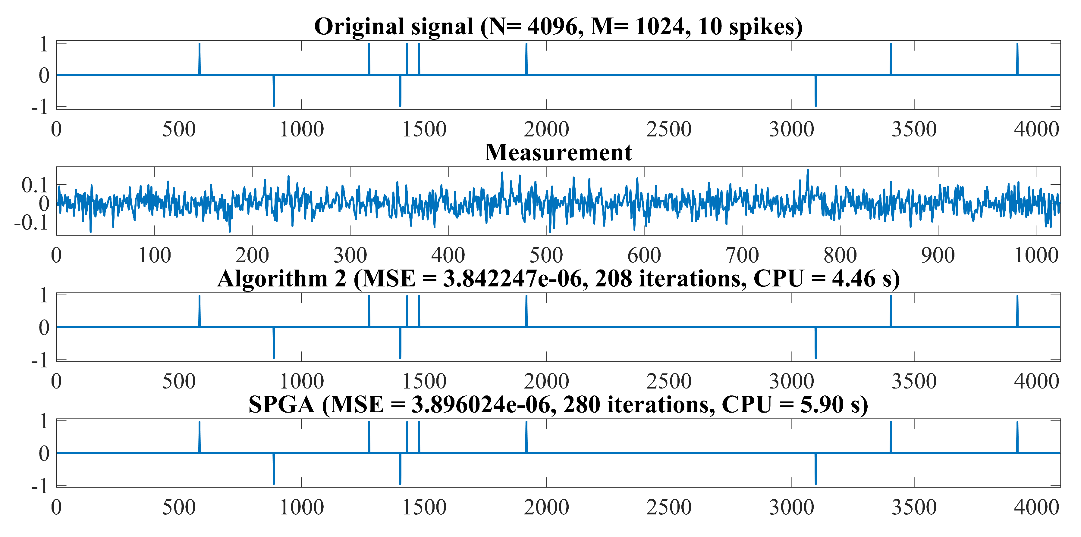
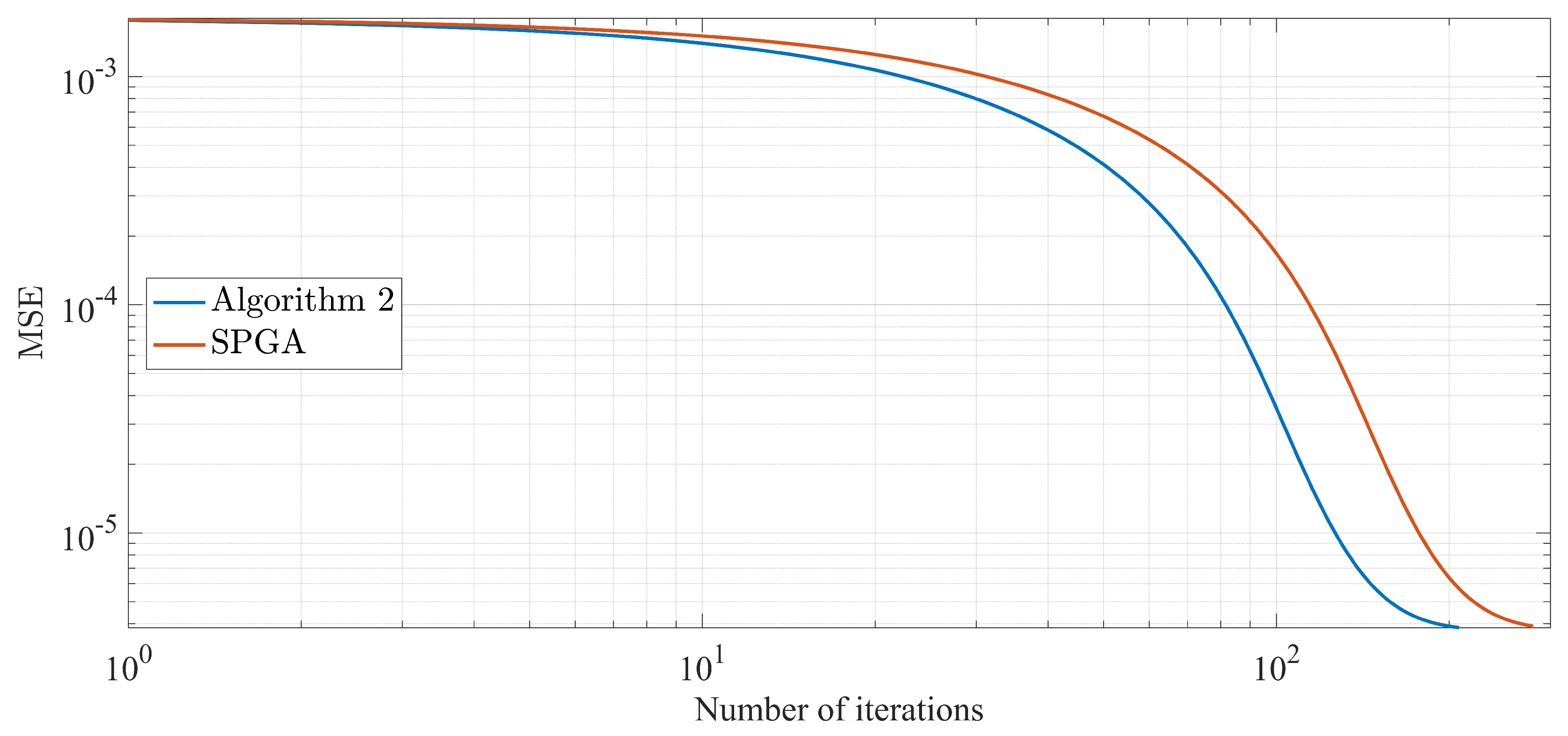
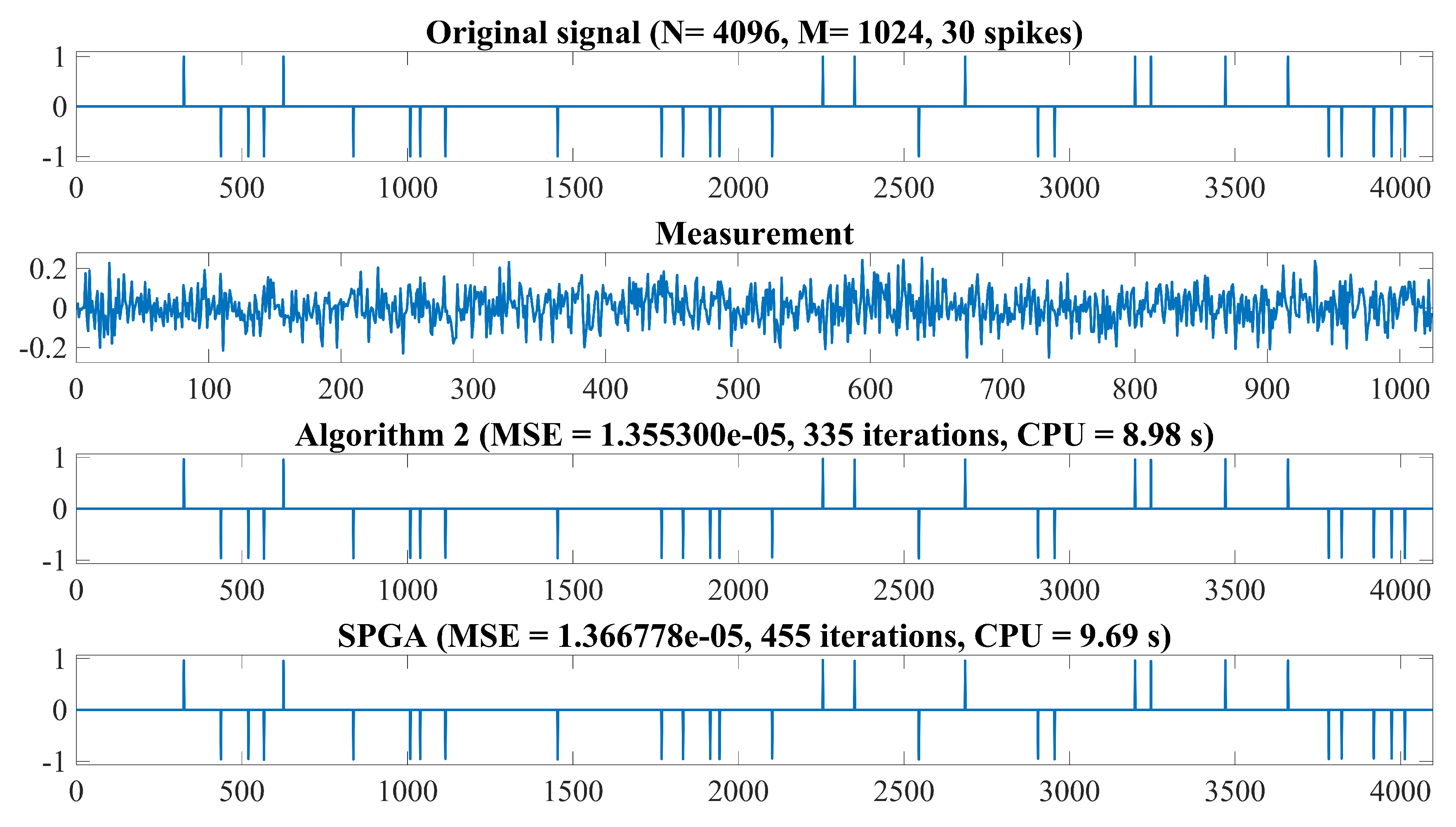
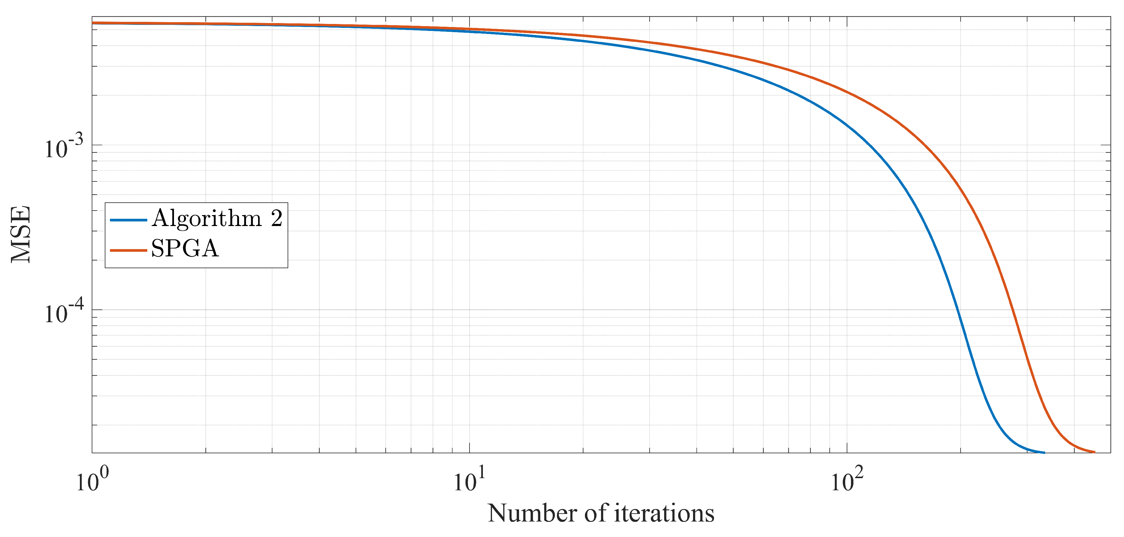
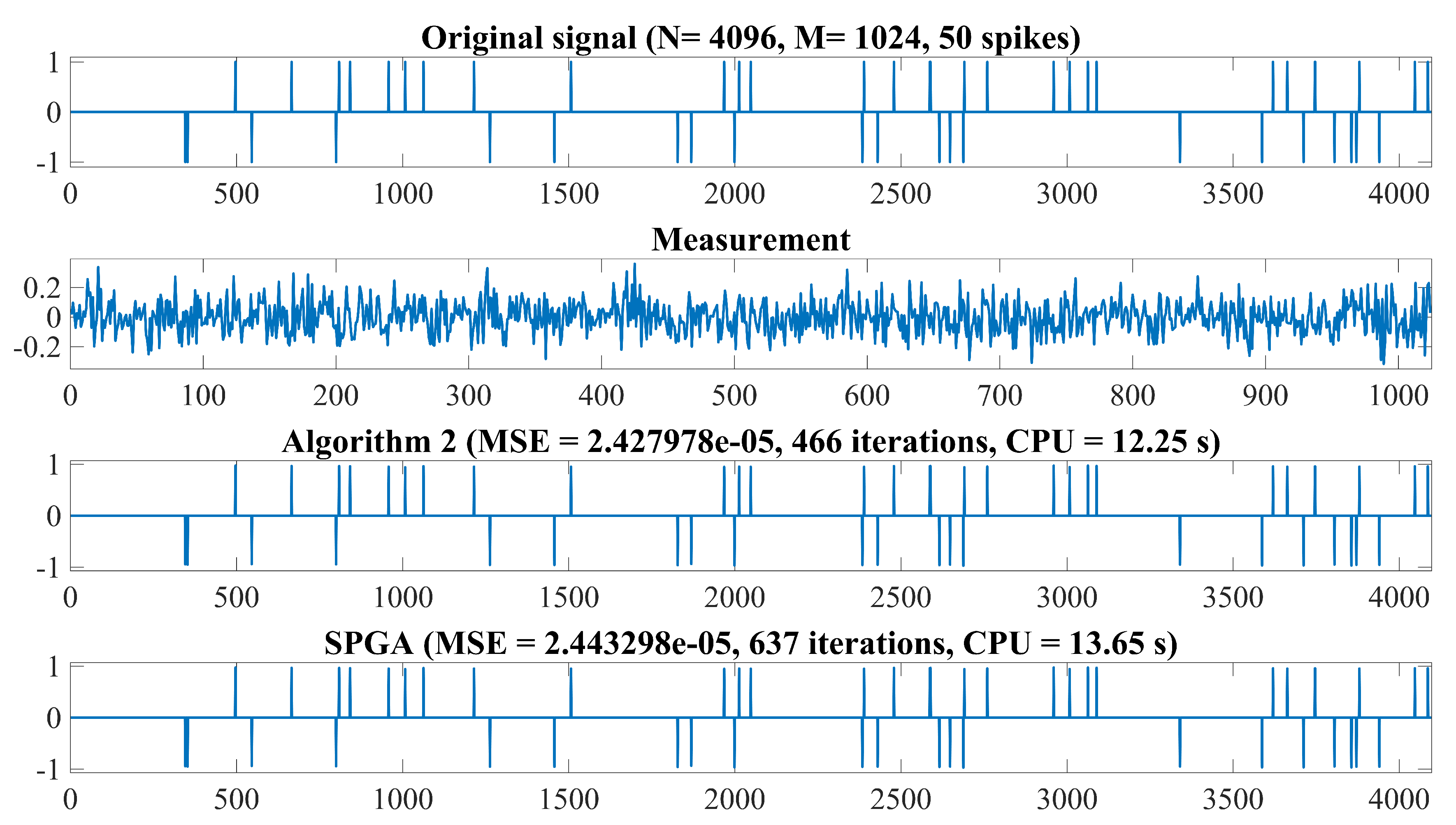
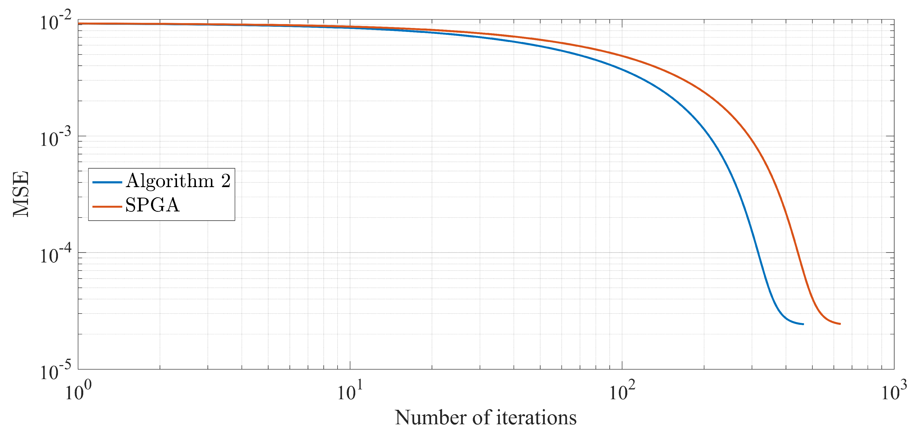
4.4. Signal Processing

We consider some applications of our algorithm to inverse problems occurring from signal processing. For example, we consider the following underdeterminated linear equation system:

$$y=\mathcal{A}u+e,$$

(21)

where $u\in {\mathbb{R}}^N$ is recovered, $y\in {\mathbb{R}}^M$ is observations or measured data with noisy e, and $\mathcal{A}:{\mathbb{R}}^N\to {\mathbb{R}}^M$ is a bounded linear observation operator. It determines a process with loss of information. For finding solutions of the linear inverse problems in Equation (21), a successful one of some models is the convex unconstrained minimization problem:

$$\underset{u\in {\mathcal{R}}^N}{min}{\displaystyle \frac{1}{2}}{\parallel \mathcal{A}u-y\parallel }^2+d{\parallel u\parallel }_1,$$

(22)

where $d>0$ and ${\parallel ·\parallel }_1$ is the $l_1–$norm. Thus, we can find solution to Equation (22) by applying our method in the case $g_1\left(u\right)=\frac{1}{2}{\parallel \mathcal{A}u-y\parallel }^2$ and $g_2\left(u\right)=d{\parallel u\parallel }_1.$ For any $\alpha \in (0,\frac{2}{\mathcal{L}}],$ the corresponding forward-backward operator $J_{\alpha }^{g_1,d{\parallel ·\parallel }_1}$ as follows:

$$J_{\alpha }^{g_1,d{\parallel ·\parallel }_1}\left(u\right)=pro{x}_{{\alpha d\parallel ·\parallel }_1}(u-\alpha \nabla g_1\left(u\right)),$$

(23)

where $g_1$ is the squared loss function of the Lasso problem in Equation (22). The proximity operator for $l_1–$norm is defined as the shrinkage operator as follows:

$$pro{x}_{{\alpha d\parallel ·\parallel }_1}\left(u\right)=max\left(\right|u_i|-\alpha d,0)·\mathrm{sgn}\left(u_i\right),$$

(24)

where $\mathrm{sgn}(·)$ is the signum function. We apply the algorithm to the problem in Equation (22) follow as Algorithm 2:

Algorithm 2: Three-step forward-backward operator

In our experiment, we set the hits of a signal $u\in {\mathbb{R}}^N$. The matrix $\mathcal{A}\in {\mathbb{R}}^{M\times N}$ was generated from a normal distribution with mean zero and one invariance. The observation y is generated by Gaussian noise distributed normally with mean 0 and variance ${10}^{-4}$. We compared our Algorithm 2 with SPGA [12]. Let ${\eta }_n={\vartheta }_n={\xi }_n=0.5,\alpha =0.1$ and $d=0.01$ in both Algorithm 2 and SPGA. The experiment was initialized by $u_1=A^{\ast }y$ and terminated when $\frac{\parallel u_{n+1}-u_n\parallel }{\parallel u_n\parallel }<{10}^{-4}.$ The restoration accuracy was measured by means of the mean squared error: MSE = $\frac{\parallel u_{\ast }{-u\parallel }^2}{N},$ where $u_{\ast }$ is an estimated signal of $u.$ All codes were written in Matlab 2016b and run on Dell i-5 Core laptop. We present the numerical comparison of the results in Figure 1, Figure 2, Figure 3, Figure 4, Figure 5 and Figure 6.

5. Conclusions

In this work, we introduce a modified iterative scheme in Banach spaces and solve common zeros of accretive operators, convexly constrained least square problem, convex minimization problem and signal processing. In the case of signal processing, all results are compared with the forward—backward method in Algorithm 2 and SPGA, as proposed in [12]. The numerical results show that Algorithm 2 has a better convergence behavior than SPGA when using the same step sizes for both.

References

1. Kankam, K.; Pholasa, N.; Cholamjiak, P. On convergence and complexity of the modified forward–backward method involving new linesearches for convex minimization. Math. Meth. Appl. Sci. 2019, 42, 1352–1362. [Google Scholar] [CrossRef]
2. Candès, E.J.; Wakin, M.B. An introduction to compressive sampling. IEEE Signal Process. Mag. 2008, 25, 21–30. [Google Scholar] [CrossRef]
3. Suantai, S.; Kesornprom, S.; Cholamjiak, P. A new hybrid CQ algorithm for the split feasibility problem in Hilbert spaces and Its applications to compressed Sensing. Mathematics 2019, 7, 789. [Google Scholar] [CrossRef]
4. Kitkuan, D.; Kumam, P.; Padcharoen, A.; Kumam, W.; Thounthong, P. Algorithms for zeros of two accretive operators for solving convex minimization problems and its application to image restoration problems. J. Comput. Appl. Math. 2019, 354, 471–495. [Google Scholar] [CrossRef]
5. Padcharoen, A.; Kumam, P.; Cho, Y.J. Split common fixed point problems for demicontractive operators. Numer. Algorithms 2019, 82, 297–320. [Google Scholar] [CrossRef]
6. Cholamjiak, P.; Shehu, Y. Inertial forward-backward splitting method in Banach spaces with application to compressed sensing. Appl. Math. 2019, 64, 409–435. [Google Scholar] [CrossRef]
7. Jirakitpuwapat, W.; Kumam, P.; Cho, Y.J.; Sitthithakerngkiet, K. A general algorithm for the split common fixed point problem with its applications to signal processing. Mathematics 2019, 7, 226. [Google Scholar] [CrossRef]
8. Combettes, P.L.; Wajs, V.R. Signal recovery by proximal forward–backward splitting. Multiscale Model Simul. 2005, 4, 1168–1200. [Google Scholar] [CrossRef]
9. Picard, E. Memoire sur la theorie des equations aux d’erives partielles et la methode des approximations successives. J. Math Pures Appl. 1890, 231, 145–210. [Google Scholar]
10. Mann, W.R. Mean value methods in iteration. Proc. Am. Math. Soc. 1953, 4, 506–510. [Google Scholar] [CrossRef]
11. Ishikawa, S. Fixed points by a new iteration method. Proc. Am. Math. Soc. 1974, 44, 147–150. [Google Scholar] [CrossRef]
12. Agarwal, R.P.; O’Regan, D.; Sahu, D.R. Iterative construction of fixed points of nearly asymptotically nonexpansive mappings. J. Nonlinear Convex Anal. 2007, 8, 61–79. [Google Scholar]
13. Sahu, V.K.; Pathak, H.K.; Tiwari, R. Convergence theorems for new iteration scheme and comparison results. Aligarh Bull. Math. 2016, 35, 19–42. [Google Scholar]
14. Thakur, B.S.; Thakur, D.; Postolache, M. New iteration scheme for approximating fixed point of non-expansive mappings. Filomat 2016, 30, 2711–2720. [Google Scholar] [CrossRef]
15. Chang, S.S.; Wen, C.F.; Yao, J.C. Zero point problem of accretive operators in Banach spaces. Bull. Malays. Math. Sci. Soc. 2019, 42, 105–118. [Google Scholar] [CrossRef]
16. Browder, F.E. Nonlinear mappings of nonexpansive and accretive type in Banach spaces. Bull. Am. Math. Soc. 1967, 73, 875–882. [Google Scholar] [CrossRef] [Green Version]
17. Browder, F.E. Semicontractive and semiaccretive nonlinear mappings in Banach spaces. Bull. Am. Math. Soc. 1968, 7, 660–665. [Google Scholar] [CrossRef]
18. Cioranescu, I. Geometry of Banach Spaces, Duality Mapping and Nonlinear Problems; Kluwer: Amsterdam, The Netherlands, 1990. [Google Scholar]
19. Takahashi, W. Nonlinear Functional Analysis, Fixed Point Theory and Its Applications; Yokohama Publishers: Yokohama, Japan, 2000. [Google Scholar]
20. Rockafellar, R.T. On the maximal monotonicity of subdifferential mappings. Pac. J. Math. 1970, 33, 209–216. [Google Scholar] [CrossRef] [Green Version]
21. Xu, H.K. Inequalities in Banach spaces with applications. Nonlinear Anal. 1991, 16, 1127–1138. [Google Scholar] [CrossRef]
22. Opial, Z. Weak convergence of the sequence of successive approximations for nonexpansive mappings. Bull. Am. Math. Soc. 1967, 73, 591–597. [Google Scholar] [CrossRef] [Green Version]
23. Sahu, D.R.; Pitea, A.; Verma, M. A new iteration technique for nonlinear operators as concerns convex programming and feasibility problems. Numer. Algorithms 2019. [Google Scholar] [CrossRef]
24. Goebel, K.; Reich, S. Uniform Convexity, Hyperbolic Geometry and Non Expansive Mappings; Marcel Dekker: New York, NY, USA; Basel, Switzerland, 1984. [Google Scholar]
Figure 1. From top to bottom: Original signal, observation data, recovered signal by Algorithm 2 and SPGA with N = 4096 , M = 1024 and 10 spikes, respectively.
Mathematics 07 00866 g001
Figure 2. Comparison MSE of two algorithms for recovered signal with N = 4096 , M = 1024 and 10 spikes, respectively.
Mathematics 07 00866 g002
Figure 3. From top to bottom: Original signal, observation data, recovered signal by Algorithm 2 and SPGA with N = 4096 , M = 1024 and 30 spikes, respectively.
Mathematics 07 00866 g003
Figure 4. Comparison MSE of two algorithms for recovered signal with N = 4096 , M = 1024 and 30 spikes, respectively.
Mathematics 07 00866 g004
Figure 5. From top to bottom: Original signal, observation data, recovered signal by Algorithm 2 and SPGA with N = 4096 , M = 1024 and 50 spikes, respectively.
Mathematics 07 00866 g005
Figure 6. Comparison MSE of two algorithms for recovered signal with N = 4096 , M = 1024 and 50 spikes, respectively.
Mathematics 07 00866 g006