1. Introduction
Reconstructing curve/surface is an important work in the field of computer aided geometric design, especially in geometric modeling and processing where it is crucial to fit curve/surface in high accuracy and reduce the error of representation curve/surface. The representation of the four curve types are the explicit-type, implicit-type, parametric-type and subdivision-type. Because implicit representation has unique advantage in the process of computer aided geometric design, it has wide and far-reaching applications. From scattered and unorganized three-dimensional data, Bajaj et al. [
1] reconstructed surface and functions on surfaces. They [
2,
3] have constructed the algebraic B-spline surfaces with least-squares fitting feature using tensor product technique. Schulz et al. [
4] constructed an enveloping algebraic surface using gradually approximate algebraization method. Kanatani et al. [
5] applied the algebraic curve to construct geometric ellipse fitting using unified strict maximum likelihood estimation method. Mullen et al. [
6] reconstructed robust and accurate algebraic surface functions to sign the unsigned from scattered and unorganized three-dimensional data point sets. Upreti et al. [
7] used a technique to sign algebraic level sets on NURBS surface and algebraic Boolean level sets on NURBS surfaces. Rouhani et al. [
8] applied the algebraic function for polynomial representation system. And L.G. Zagorchev et al. [
9] applied the algebraic function for general algebraic surface.
Up to now, there are three main types of methods to solve the problem of point orthogonal projection onto planar algebraic curve: local method, global method and compromise method between these two methods. Here are three typical approaches.
According to the most basic geometric characteristic, orthogonal projection of test point
onto the planar algebraic curve is actually the point
on the curve such that cross product of vectors
and
is 0.
Equation (
1) can be transformed into Newton’s iteration formula (3). Furthermore, Sullivan et al. [
10] adopted a hybrid method with Lagrange multiplier and Newton’s iterative method to compute the closest point on the planar algebraic curve for each test point. Some orthogonal projection problems can be transformed into solving system of nonlinear equations. The common characteristic of methods [
10,
11] is that they converge locally and fast, while methods [
10,
11] are dependent on the initial points.
The first global method of solving system of nonlinear equations is the Homotopy continuous method [
12,
13]. They constructed Homotopy continuous formula.
where
t is a parameter of continuous transformation from 0 to 1,
is the original system of nonlinear equations to be solved,
is the objective solution of system of nonlinear equations
. All isolated solutions of system of nonlinear equations
can be computed by the numerical continuous Homotopy methods [
12,
13]. So the Homotopy methods [
12,
13] are global convergence. The Homotopy methods’ robustness is proved by [
14] and their high time-consuming property is verified in [
15]. Of course, the Homotopy methods [
12,
13] are ideal in theory, but it is difficult to find or construct the objective system of nonlinear equations
in practical engineering applications.
The second global resultant methods convert system of nonlinear equations into the expression of the resultants and then solve the resultants [
16,
17,
18,
19]. According to classical elimination theory, system of two nonlinear equations with two variables can be turned into a resultant polynomial with one variable, which is equivalent to the two simultaneous equations. The Sylvester’s resultant and Cayley’s statement of Bézout’s method are the most famous resultant methods [
16,
17,
18,
19]. Because the resultant methods [
16,
17,
18,
19] can solve all roots if the degree of the planar algebraic curve is less than 4, they are good global methods. However, if the degree of the planar algebraic curve is more than quintic, it becomes harder and harder with increasing degree to solve two-polynomial system with the resultant methods.
The third global method is the adoption of the Bézier clipping technique [
20,
21,
22]. In the first step, solving the nonlinear system of Equation (
1) is transformed into solving all roots of Bernstein-Bézier representation with convex hull property. In the second step, if the parts of the domains do not include the solution, we clip the parts of the domains by using convex hull box with Bernstein-Bézier form such that the discarded parts of the region has no solution and all the solutions are in the retained parts of the region. In the third step, the de Casteljau subdivision rule is used to segment the remaining part of the curve obtained by elimination in step 2. Repeat steps 2 and 3 until we can find all the solutions to Equation (
1). The advantage of this method is that all solutions of Equation (
1) can be found. But this global clipping method has one difficulty: sometimes Equation (
1) is difficult or even impossible to convert into Bernstein-Bézier form. For example, specific Equation (
1)
is impossible to convert into Bernstein-Bézier form where
.
The compromise method is between local and global methods. Consisting of the geometric property with computing the nearest point is proposed by Hartmann [
23,
24] named as the first compromise method. Repeatedly run the Newton’s steepest gradient descent method (3) until the iterative point falls on the planar algebraic curve, where the initial iterative point is unrestricted.
Running the iterative formula (4) one time, the method [
23,
24] can obtain the vertical foot point
where the iterative point
of the formula (4) is the final iterative point obtained by formula (3). Continuously iterate the above two steps until the vertical foot point
is on the planar algebraic curve
. Unluckily, progressive geometric tangent approximation iteration method with computing vertical foot point
fails for some planar algebraic curves
.
The second compromise method is developed by Nicholas [
25] who adopted the osculating circle technique to realize orthogonal projection onto the planar algebraic curve. Calculate the corresponding curvature at one point on the planar algebraic curve, and then the radius and center of the curvature circle. The line segment formed by the test point and the center of the curvature circle intersects the curvature circle at footpoint
. Approximately take the footpoint
as a point on the planar algebraic curve. For the new point on the planar algebraic curve, repeat the above procedure to get a new footpoint and corresponding new approximate point on the planar algebraic curve. Repeat the above behavior until the footpoint
is the orthogonal projection point
. Because the planar algebraic curve does not have parametric control like parametric curve, taking the footpoint as an approximate point on the planar algebraic curve will bring about large errors. So it makes the operation of the whole algorithm unstable.
The third compromise method is the circle shrinking technique [
26]. Repeatedly run the iterative formula (3) such that the final iterative point
falls on the planar algebraic curve as far as possible, where the selection of initial iterative point is arbitrary. The next iterative point on the planar algebraic curve is obtained through a series of combined operations of circle and the planar algebraic curve, where the center and radius of the circle are test point
and
, respectively. A series of combined operations include the two most important steps: Find a point
on the circle by means of the mean value theorem; Seek the intersection of the line segment
and the circle where we call this intersection as the current intersection point
. Repeatedly run this series of combined operations until the distance between the current point
and the previous point
is 0. The circle shrinking technique [
26] takes a lot of time to seek point
each time. The algorithm has one difficulty: if the degree of the planar algebraic curve is higher than 5, the intersection point
of line segment
and the planar algebraic curve cannot be solved directly by formula or the iterative methods to find the intersection
will lead to instability.
The four compromise method is a circle double-and-bisect algorithm [
27]. The circle doubling algorithm begins with a very small circle where the center is the test point
and the radius is very small
. Keep the same center of the circle, take the radius
twice of
to draw a new circle. If there is no intersection between the new circle and the curve, draw a new circle with radius twice of
. Continuously repeat the above process until new circle can intersect with the planar algebraic curve and the former circle does not. Naturally, the former circle and the current circle are called interior circle and exterior circle, respectively. Moreover, the bisecting technology implements the rest of the process. Continue to draw a new circle with new radius
. If the new current circle whose radius is
r intersects with the curve, substitute
r for
, else for
. Repeatedly run the above progress until the difference between the two radii is approximate zero(
. But this method is very difficult to judge whether the exterior circle intersects the planar algebraic curve or not [
27].
The fifth compromise method is the integrated hybrid second order algorithm [
28]. It includes two sub-algorithms: the hybrid second order algorithm and the initial iterative value estimation algorithm. They mainly exploint three ideas: (1) the tangent orthogonal vertical foot method coupled with calibration method; (2) Newton’s steepest gradient descent iterative method to impel the iteration point to be on the planar implicit curve; (3) Newton’s iterative method to speed up the whole iteration process. Before running the hybrid second order algorithm, the initial iterative value estimation algorithm is used to force the initial iterative value of the formula (17) of the hybrid second order algorithm and the orthogonal projection point
as close as possible. After a lot of tests, if the distance between the test point
and the curve is not very far, the advantages of this algorithm are obvious in term of robustness and efficiency. But when the test point is very far from the curve, the integrated hybrid second order algorithm is invalid.
2. The Improved Curvature Circle Algorithm
In Reference [
28], when the test point
is not particularly far away, the integrated hybrid algorithm can have ideal result. But if the test point
is very far from the curve, the algorithm is invalid where the test point
can not be robustly and effectively orthogonally projected onto the planar algebraic curve. In order to overcome this difficulty, we propose an improved curvature circle algorithm to ensure robustness and effective convergence with the test point
being arbitrarily far away. No matter how far the test point
is from the planar algebraic curve, if the initial iteration point
is very close to the orthogonal projection point of the test point
, the preconceived algorithm can converge well. So we attempt to construct an algorithm to find an initial iterative point very close to the orthogonal projection point
of the test point
. The general idea is the following. Repeatedly iterate the formula (3) by utilizing the Newton’s steepest gradient descent method until the iteration point fall on the planar algebraic curve as far as possible, written as
. This time, the distance between the iteration point
and the orthogonal projection point
is much smaller than that between the original iteration point
and the orthogonal projection point
. The iteration point
is closer to the orthogonal projection point
. In order to further promote the iteration point
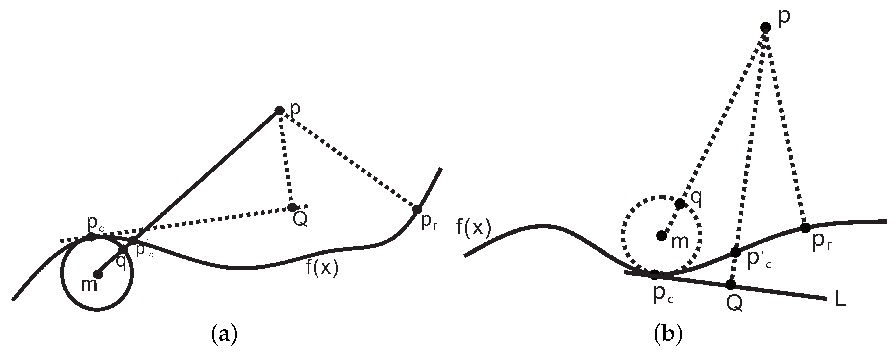
and the orthogonal projection point
to be closer, we introduce a key step with curvature circle algorithm. Draw a curvature circle through point
on the planar algebraic curve with the radius
R determined by the curvature
k and the center
being a normal direction point of point
on the planar algebraic curve. Line segment
determined by the test point
and the center
intersects curvature circle at point
. We take the intersection point
as the next iteration point for the iteration point
. Of course, the distance between the intersection point
and the orthogonal projection point
is much smaller than the previous one. We use the intersection point
as the new test point, and run the hybrid algorithm again where the initial iterative point at this moment can be set as
. Repeatedly iterate until the iteration point falls on the planar algebraic curve
, written as
. We repeat the last two key steps in this procedure until the iteration point
and the orthogonal projection point
overlap (See
Figure 1).
Let’s elaborate on the general idea. Let
be a test point on the plane. There is an planar algebraic curve
on the plane.
The plane algebraic curve (5) can be simply written as
where
. The goal of this paper is to find a point
on the planar algebraic curve
to satisfy the basic relationship
The above problem can be written as
where
is Hamiltonian operator and symbol × is cross product. We take
s as the arc length parameter of the planar algebraic curve
and
is unit tangent vector along the planar algebraic curve
. Take derivative of Equation (
6) with respect to arc length parameter
s and combine with unit tangent vector condition
, we obtain the following simultaneous system of nonlinear equations,
It is easy to get the solution of Equation (
9).
Repeatedly iterate Equation (
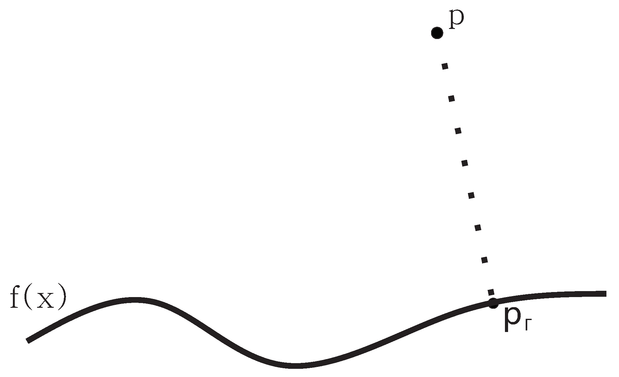
3) called as the Newton’s steepest gradient descent method until until the iterative termination criteria
, where the initial iterative point is
and refer to the iterative point
as
. The first advantage of the Newton’s steepest gradient descent method (3) is to make the iteration point fall on the planar algebraic curve
as far as possible. Its second advantage of the Newton’s steepest gradient descent method (3) is that the iteration point fallen on the planar algebraic curve is relatively close to the orthogonal projection point
, and it brings great convenience to implementation of the subsequent sub-algorithms. The Newton’s steepest gradient descent method (Algorithm 1) can be specifically described as (See
Figure 2).
| Algorithm 1: The Newton’s steepest gradient descent method. |
Input: The test point p and the planar algebraic curve
Output: The iterative point fallen on planar algebraic curve
Description:
Step 1:
;
Do {
;
Update according to the iterative Equation (3);
}while (;
Step 2:
;
Return ; |
In this case, if the iterative point
fallen on the planar algebraic curve
is taken as the initial iterative point of the hybrid algorithm, convergence or divergence may occur where divergence can not improve the algorithm. As for divergence, it can not achieve the purpose of improving the algorithm. From another point of view, the distance between iteration point
and orthogonal projection point
of the test point
should be closer. It lays a good foundation for the implementation of subsequent sub-algorithms. In order to get the iteration point and the orthogonal projection point
closer, we adopt curvature circle way to promote the iteration point and the orthogonal projection point
being closer. Because the iterative point is on the planar algebraic curve, the curvature
k at the iterative point
fallen on the planar algebraic curve
is defined as [
29],
where
. The radius
R and the center
of the curvature circle ◯ directed by the curvature
k are
and
where the unit normal vector
is
. The line segment
determined by the test point
and the center
of the curvature circle ◯ intersects the curvature circle ◯ at point
which is named as footpoint
. From elementary geometric knowledge, the parametric equation of the line segment
can be expressed as
where parametric
is undetermined. In addition, the equation of the curvature circle ◯ can be written as
By solving Equation (
14) and Equation (
15) together, the analytic expression of the intersection
is obtained
where the undetermined parameter
w is accurately identified as
. The computation of the footpoint
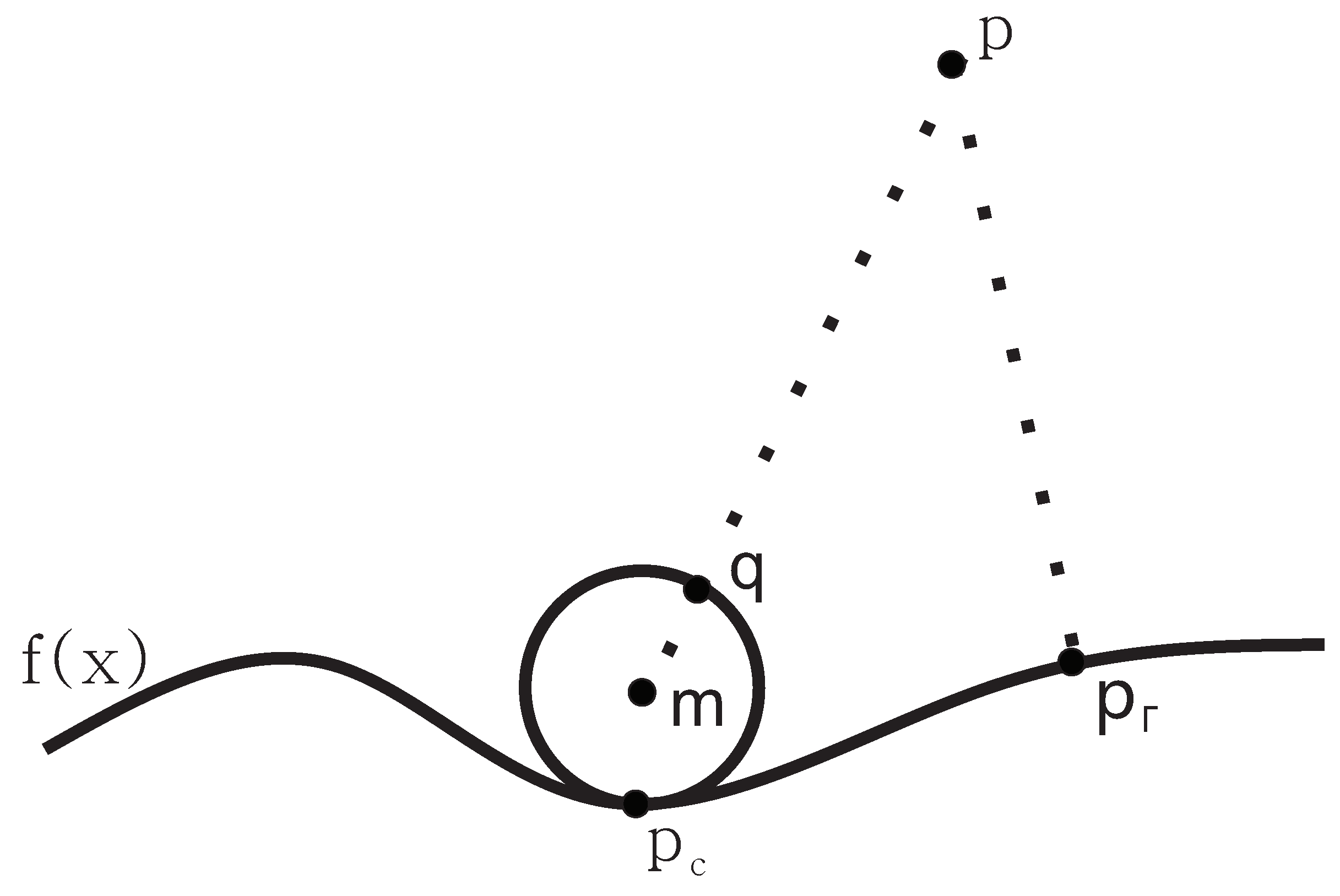
can be realized through Algorithm 2 (See
Figure 3).
| Algorithm 2: Computing footpoint via the curvature circle ◯ and the line segment . |
Input: The test point , the planar algebraic curve and the iterative point on the
planar algebraic curve .
Output: The footpoint .
Description:
Step 1:
Compute the curvature k of the iterative point fallen on the planar algebraic curve
by the curvature calculation formula (11).
Step 2:
Calculate the radius R and the center of the curvature circle ◯ through the formulas
(12) and (13), respectively.
Step 3:
Compute the footpoint by the formula (16).
Return ; |
Remark 1. The important formula for computing the curvature k is the formula (11). If the denominator of the curvature k with the formula (11) is 0, the whole iteration process will degenerate. In order to solve this special degeneration, we adopt a small perturbation of the curvature k of the formula (11) in programming implementation of Algorithm 2. Namely, the denominator of the curvature k with the formula (11) could be incremented by a small positive constant ε, the denominator of the curvature k is the denominator of the curvature k +ε, and Algorithm 2 continues to calculate the center and the radius of the curvature circle corresponding to the curvature after disturbance. Of course, in all subsequent formulas or iterative formulas, we also do the same denominators perturbation treatment for the case of the zero denominators of the formulas or the iterative formulas.
Under this circumstance, if the footpoint point
at this moment is taken as the initial iteration point of the hybrid algorithm, the convergence probability of the hybrid algorithm is much greater than that of using the point
in Algorithm 1 as the initial iterative point of the hybrid algorithm. The reason is that the distance
is smaller than the distance
. But divergence may happen in this case. In order to further guarantee the robustness,we orthogonally project the footpoint
onto the planar algebraic curve
by using the hybrid algorithm, instead of directly using the footpoint
q as the initial iterative point. At this time we still call the orthogonal projection point of the footpoint
as the point
which is just fallen on the planar algebraic curve
. Because at this time the footpoint
is close to the planar algebraic curve
, the algorithm can ensure complete convergence. The distance between the iterative point
and the orthogonal projection point
of the test point
becomes smaller again. The core iterative formula (17) of the hybrid algorithm is as follows (See [
28]).
where
,
,
,
,
,
.
The iterative formula (17) mainly contains four techniques. The core technology is the tangent foot vertical method with the third step and the fourth step of the iterative formula (17). Draw a tangent line from a point on a plane algebraic curve . Through the footpoint (The footpoint at this time is as the test point of iterative formula (17)), make a vertical line of the tangent and get its corresponding vertical foot point , which is equivalent to the third step in the formula (17). From the fourth step of the iterative formula (17), we get the next iteration point of particular importance for the initial iteration point. When the next iteration point is not very close to the planar algebraic curve , we adopt the second important technique with the iteration point correction method, equivalent to the sixth step of the iterative formula (17). The iteration point is to move to the plane algebra curve as close as possible such that the distance between the correction point of the iteration point and the plane algebra curve is as close as possible. These two techniques are pure geometric techniques. When the distance between the test point and the planar algebraic curve is very close, the effect of convergence is obvious. Of course, when the distance between the test point and the planar algebraic curve is relatively long, sometimes there will be non-convergence. In order to improve the robustness of convergence, we add the Newton’s steepest gradient descent method before the first technique with the third step and the fourth step of the iterative formula (17). Its first aim is to bring the initial iteration point closer to the planar algebraic curve . Its second aim is to promote the accuracy of subsequent iterations. In order to accelerate the whole iteration process of the iterative formula (17), we once again incorporate the fourth technology of Newton’s iterative method which is closely related to the footpoint . This technique not only accelerates the convergence rate of the whole iteration process but also improves the iteration robustness. Furthermore, the accuracy of the whole iteration process can be improved by the fourth technique. So we add Newton’s iterative method after the first step with the second technique, and then add it again before the last step with the third technique. Based on the above explanation and illustration, we get the following the hybrid tangent vertical foot algorithm (Algorithm 3).
| Algorithm 3: The hybrid tangent vertical foot algorithm (See Figure 4). |
Input: The footpoint and the planar algebraic curve .
Output: The point fallen on the planar algebraic curve .
Description:
Step 1:
;
Do {
;
Execute according to the iterative Equation (17);
}while (&&
Step 2:
;
Return ; |
With the description of the above three algorithms, we propose a comprehensive and complete algorithm (Algorithm 4) closely related to Algorithm 2 (See
Figure 4).
| Algorithm 4: The first improved curvature circle algorithm (Comprehensive Algorithm A). |
Input: Test point and the planar algebraic curve .
Output: Orthogonal projection point of the test point which orthogonally projects the test
point onto a planar algebraic curve .
Description:
Step 1:Starting from the neighbor point of the test point , calculate the point fallen on the
via Algorithm 1.
Do{
Step 2: Compute the footpoint via Algorithm 2.
Step 3: Project footpoint onto the planar algebraic curve via Algorithm 3, then get
the new iterative point fallen on the .
}while (distance (the current , the previous )).
;
Return ; |
Through a series of rigorous deductions, Comprehensive Algorithm A is the important algorithm of our paper. No matter how far the test point
is from the planar algebraic curve
, test point
could very robustly orthogonally projects onto the planar algebraic curve
. This has achieved our desired result. After a lot of testing and observation, when the point on the curve is close to the orthogonal projection point, we find that Comprehensive Algorithm A presents two characteristics: (1) difference between the first distance and the second distance decreases slower and slower, where the first distance and the second distance are the one between the previous iterative point
on the planar algebraic curve and the orthogonal projection point
, and the one between the current iterative point
on the planar algebraic curve and the orthogonal projection point
, respectively; (2) the rate goes even slower at which the absolute value of the inner product gradually approaches zero. These two characteristics are what we don’t want to obtain because they are contrary to the efficiency of computer systems. On the premise of ensuring robustness, we try our best to improve and excavate a certain degree of efficiency for the problem of point orthogonal projection onto planar algebraic curve. We have an ingenious discovery. After each running of Algorithm 3, we run the Newton’s iterative method associated with the original test point
, which can improve the convergence and ensure the orthogonality. Namely, that is to add this step after the last step of the formula (17). Thus the iterative formula (18) is obtained.
where
,
,
,
,
,
,
,
. Because the iterative formula (17) of Algorithm 3 naturally becomes the iterative formula (18), so Algorithm 3 naturally becomes the following Algorithm 5.
| Algorithm 5: The hybrid tangent vertical foot algorithm. |
Input: The footpoint and the planar algebraic curve .
Output: The point fallen on planar algebraic curve .
Description:
Step 1:
;
Do {
;
Execute according to the iterative Equation (18);
}while (&&
Step 2:
;
Return ; |
Now let’s replace Algorithm 3 of Comprehensive Algorithms A with Algorithm 5. We get the following Comprehensive Algorithm B (Algorithm 6).
| Algorithm 6: The second improved curvature circle algorithm (Comprehensive Algorithm B). |
Input: Test point and the planar algebraic curve .
Output: Orthogonal projection point of the test point which orthogonally projects the test
point onto the planar algebraic curve .
Description:
Step 1: Starting from the neighbor point of the test point , calculate the point fallen on the via Algorithm 1.
Do{
Step 2: Compute the footpoint via Algorithm 2.
Step 3: Project footpoint onto the planar algebraic curve via Algorithm 5, then get
new point fallen on the .
}while(distance(the current , the previous )).
;
Return ; |
Comprehensive Algorithm A and Comprehensive Algorithm B share common advantage: the robustness of the two algorithms is substantially improved than that of the existing algorithms because our algorithms are not subject to any restrictions on test points and initial iteration points. By comparison, Comprehensive Algorithm B has four advantages over Comprehensive Algorithm A. (1) The last step of the iterative formula (18) in Comprehensive Algorithm B can make corrections continuously; (2) The last step of the iterative formula (18) in Comprehensive Algorithm B accelerates the whole Comprehensive Algorithm B; (3) The last step of the iterative formula (18) in Comprehensive Algorithm B accelerates the inner product of two vectors to 0, where the first vector refers to the vector connecting the test point and the iteration point of Comprehensive Algorithm B and the second vector is the tangent vector derived from the iteration point on the planar algebraic curve, respectively; (4) Comprehensive Algorithm B overcomes two shortcomings of Comprehensive Algorithm A.
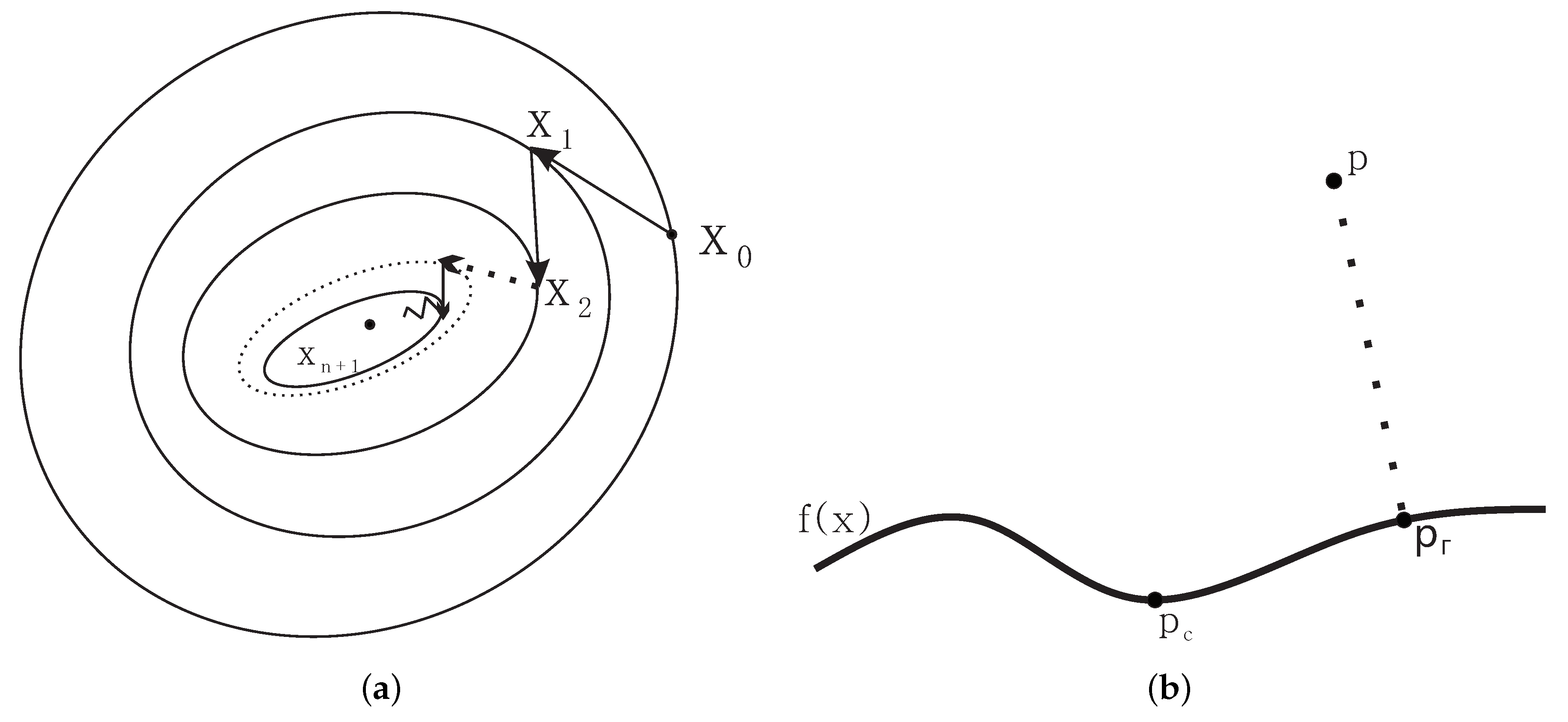
Of course, when the test point is not too far from the plane algebra curve, Comprehensive Algorithm is also convergent for any initial iterative point. However, Comprehensive Algorithm A takes more time than directly using the hybrid second order algorithm. In practical applications such as computer graphics, it’s hard to know if the test point is close to or far from a planar algebraic curve. Because the main reason is that the degree and the type of the planar algebraic curve restrict the relative distance between the test point and the planar algebraic curve. In order to optimize time efficiency, we take advantage of Comprehensive Algorithm A and the hybrid second order algorithm such that no matter where the test point is located, it can be orthogonally projected onto the planar algebraic curve efficiently and robustly. First, the hybrid second order algorithm is iterated. If it does not converge after 100 iterations, it will be changed to Comprehensive Algorithm A to iterate until the iteration point reaches the orthogonal projection point . Specific algorithm implementation is the following Comprehensive Integrated Algorithm A (Algorithm 7).
| Algorithm 7: The first comprehensive integrated improved curvature circle algorithm (Comprehensive Integrated Algorithm A). |
Input:Test point and the planar algebraic curve .
Output: Orthogonal projection point of the test point .
Description:
Step 1:
;
for() {
;
=Hybrid second order algorithm;
if break ;
}
Step 2:
if( {
;
=Comprehensive Algorithm A;
}
;
Return ; |
Number N is an empirical value of the iterative times where the value N is specified as 5 or 6.
Similar to Comprehensive Algorithm A, by replacing Algorithm 3 with Algorithm 5, the following Comprehensive Integrated Algorithm B (Algorithm 8) can be obtained naturally.
| Algorithm 8: The second comprehensive integrated improved curvature circle algorithm (Comprehensive Integrated Algorithm B). |
Input: The test point and the planar algebraic curve .
Output: Orthogonal projection point of the test point .
Description:
Step 1:
;
for() {
;
=Hybrid second order algorithm;
if break ;
}
Step 2:
if( {
;
=Comprehensive Algorithm B;
}
;
Return ; |
Number N is an empirical value of the iterative times where the value N is specified as 5 or 6.
To sum up, we have presented four synthesis algorithms altogether. After analysis and judgment, Comprehensive Algorithm B and Comprehensive Integrated Algorithm B are the most robust and efficient. On the problem of orthogonal projection of point onto planar algebraic curve, if the distance between the test point and the planar algebraic curve is close, we recommend the hybrid second order algorithm, if the distance between the test point and the planar algebraic curve is not close, we recommend Comprehensive Algorithm B. Of course, if the distance between the test point and the planar algebraic curve cannot be known to be very far or close, Comprehensive Integrated Algorithm B is the best choice.
Remark 2. In sum, Comprehensive Algorithm B has strong superiority over existing algorithms [10,11,12,13,14,15,16,17,18,19,20,21,22,23,24,25,26,27,28]. If the distance between the test point and the planar algebraic curve is very far away, the test point can be ideally orthogonally projected onto the planar algebraic curve. But when there are singular pointsin the planar algebraic curve, this case will seriously hinder the correct execution and implementation of Comprehensive Algorithm B. In order to solve the problem in the case of singularities in the planar algebraic curves, we propose a remedy to Comprehensive Algorithm B (Algorithm 9). The specific description is as follows (See Figure 5). | Algorithm 9: The first remedial algorithm of Comprehensive Algorithm B. |
Input: Test point and the planar algebraic curve .
Output: Orthogonal projection point of the test point .
Description:
Step 1.
Starting from the neighbor point of the test point , calculate the iterative point fallen
on the planar algebraic curve via Algorithm 1.
Step 2.
Judge whether to use curvature circle method or tangent method in the next step.
Step 3.
Find the left endpoint on the other side of relative to the test point . According
to the result of step 2, if use curvature circle method, then the left endpoint is equal to the
intersection point which is computed by the curvature circle method with the formula (16).
If not, then the left endpoint is equal to the vertical foot which is computed by the
tangent method with the third step of the formula (17).
Step 4.
Calculate the intersection point of the line segment connecting the current left
endpoint and the test point and the planar algebraic curve by the hybrid method of
combining Newton’s iterative method and binary search method. The intersection point is
called as the current iterative point ;
Step 5.
Repeat Step 2,Step 3 and Step 4 until the distance between the current iterative point
and the previous iterative point is near zero;
Step 6.
= ;
Return ; |
Now let’s describe the hybrid method of combining Newton’s iterative method and binary search method in detail. The parameter equation of the line segment
can be expressed as
where
,
, and
is a parameter of Equation (
19). Substitute Equation (
19) into Equation (
6) of the planar algebraic curve to get a equation on the parameter
w,
where the
x and
y of Equation (
20) are completely determined by the
x and
y of Equation (
19). So the most basic Newton’s iterative formula corresponding to Equation (
20) is not difficult to write as,
where
is the first derivative of
about the parameter
w. Now we start to iterate the Newton’s iterative formula (21) with the initial iterative value
. Based on the actual situation, the intersection of the line segment
and the planar algebraic curve is much closer to the left endpoint
and much farther from the original test point
, therefore, the initial interval of the binary search method can be specified as
. The detailed description of the hybrid method of combining Newton’s iterative method and binary search method is as following Algorithm 10.
| Algorithm 10: The hybrid method of combining Newton’s iterative method and binary search method. |
Input: The planar algebraic curve , the original test point , the iterative point via Algorithm 1.
Output: The intersection between the line segment and the planar algebraic curve .
Description:
Step 1:
The initial interval of the binary search method , the initial iterative
value ;
Step 2:
;
kmin=min(,);
kmax=max(,);
if ( < kmin or > kmax)
;
=sign();
=sign();
if()
;
else
;
Step 3:
Repeatedly iterate Step 2 until ;
Step 4:
;
Return ; |
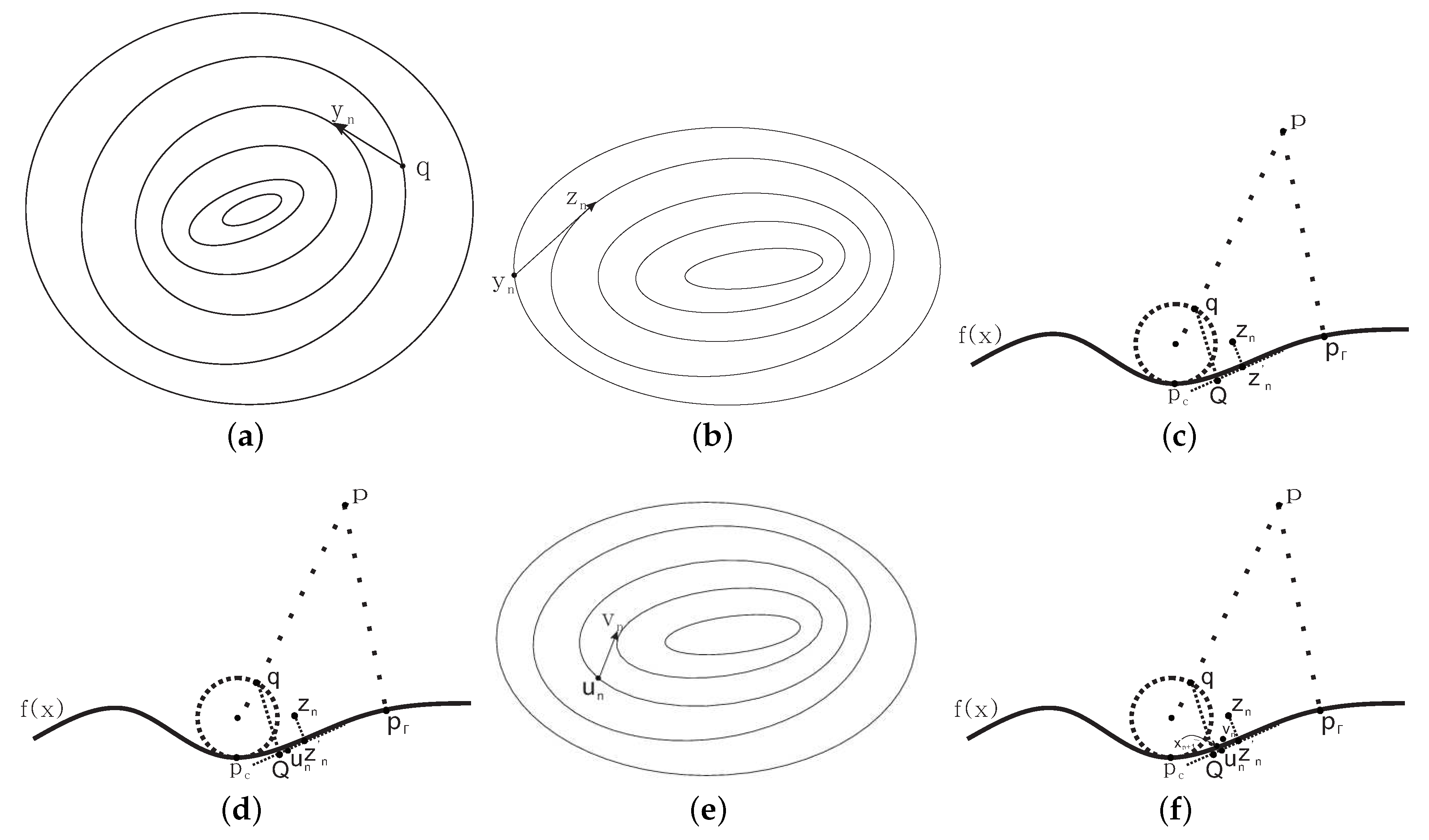
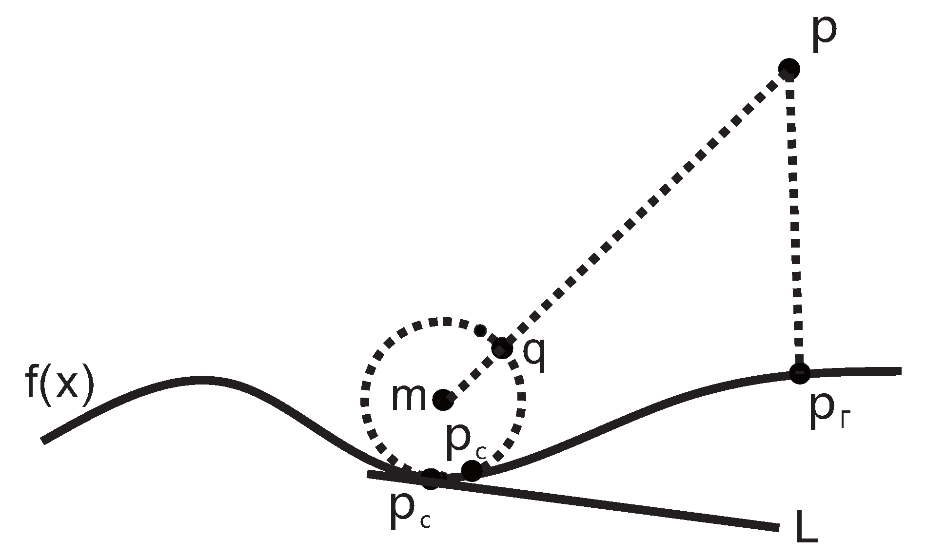
The robustness of the first remedial algorithm of Comprehensive Algorithm B is much better than that of Comprehensive Algorithm B while the first remedial algorithm of Comprehensive Algorithm B takes much more time than Comprehensive Algorithm B. The hybrid method of combining Newton’s iterative method and binary search method is a hybrid method which binary search method ensures global convergence and the Newton’s iterative method plays an accelerating role. In order to ensure robustness and improve efficiency, we have fully excavated Comprehensive Algorithm B. We have developed Second Remedial Algorithm (Algorithm 11). The specific description is as follows (See
Figure 6).
| Algorithm 11: Second Remedial Algorithm. |
Input: Test point and the planar algebraic curve .
Output: Orthogonal projection point of the test
point which orthogonally projects the test point onto the planar algebraic curve
Description:
Step 1: Starting from a certain percentage of the test point , calculate the point fallen on the
via Algorithm 1.
Do{
Step 2: Compute the footpoint via Algorithm 2.
Step 3: Starting from the footpoint , compute the iterative point fallen on the via
Algorithm 1.
}while(distance(the current , the previous )).
Step 4: Compute the orthogonal projection point of the test point via Algorithm 12.
Return ; |
| Algorithm 12: The hybrid Newton-type iterative algorithm. |
Input: The current iterative point fallen on the planar
algebraic curve and the planar algebraic curve .
Output: Orthogonal projection point of the test point which orthogonally projects the test
point onto the planar algebraic curve .
Description:
Step 1:
;
Do {
;
Compute according to the iterative formula (22);
}while (&&
Step 2:
;
Return ; |
The expression of the iterative formula (22) is as follow,
where
,
,
,
.
Remark 3. In this remark, we present the geometric interpretation of Second Remedial Algorithm. The purpose of the first step is to make the iterative pointfall on the planar algebraic curve as much as possible through Newton’s steepest gradient descent method of Algorithm 1, where the coordinates of the initial iterative point take proportional value of that of the test pointto ensure that Algorithm 1 converges successfully. Otherwise, the distance between the initial iterative point and the planar algebraic curve is very large, which easily leads to the divergence of Algorithm 1. The purpose of Do … While cycle body in Second Remedial Algorithm is to continuously and gradually move the iterative pointto fall on the planar algebraic curve to the orthogonal projection point. The second step inDo … Whilecycle body in Second Remedial Algorithm has two characteristics. Since the footpointis the unique intersection point of the curvature circle and the straight line segmentconnecting the centreof the curvature circle and the test point, the footpointis always closely related to the iterative pointfallen on the planar algebraic curve and the test point. The first characteristic is that the footpointcan guarantee the global convergence of the whole algorithm (Second Remedial Algorithm). The second characteristic is that the distance between the footpointand the planar algebraic curve is much smaller than the distance between the test pointand the planar algebraic curve. So the third step with Algorithm 1 in Do… Whilecycle body can very robustly iterate the footpointonto the planar algebraic curve. The core thought of Do … While cycle body in Second Remedial Algorithm is to keep the iterative pointto fall on the planar algebraic curve and to move towards the orthogonal projection pointsuch that the distancebetween the iterative pointand the orthogonal projection pointbecomes smaller and smaller. As the distancegets smaller and smaller, we have found that there is a defect in Do … While cycle body in Second Remedial Algorithm. The decreasing speed of the distanceis getting slower and slower. Especially the second formula of the formula (8) is very difficult to be satisfied. Namely, it is difficult to orthogonalize the vectorand the vector. In order to overcome the difficulty, we add Algorithm 12 behind Do … While cycle body in Second Remedial Algorithm. Algorithm 12 includes three components: (1) The Newton’s steepest gradient descent method in the first step; (2) The Newton’s iterative method closely associated with the test pointin the second step; (3) Correcting method in the third step. Algorithm 12 has four advantages and important roles: (1) Algorithm 12 plays a role for accelerating the whole algorithm (Second Remedial Algorithm); (2) The first step plays a role for making the iteration point fall on the planar algebraic curve as far as possible; (3) The second step plays a role for accelerating orthogonalization between the vectorand the vector; (4) The third step plays a dual role for the accelerating orthogonalization and the promoting the iterative point to fall on the planar algebraic curve. The numerical tests of Second Remedial Algorithm achieve our expected results. No matter how far the test pointis from the planar algebraic curve, Second Remedial Algorithm can converge very robustly and efficiently. Second Remedial Algorithm is the best one in our paper. Of course, the robustness and the efficiency of Second Remedial Algorithm are better than that of the existing algorithms. We are very happy about that.
Remark 4. In order to further improve the efficiency of the test pointorthogonal projecting onto plane algebraic curve, we construct a Comprehensive Integrated Algorithm C which includes two parts: the hybrid second order algorithm in [28] and Second Remedial Algorithm. Firstly run the hybrid second order algorithm in [28]. If the hybrid second order algorithm converges, then it means that Comprehensive Integrated Algorithm C is finished. Otherwise, Second Remedial Algorithm runs until it converges successfully. That is the end of Comprehensive Integrated Algorithm C. The specific description of Comprehensive Integrated Algorithm C is similar to that of Comprehensive Integrated Algorithm B. Here, we are not giving a detailed description of Comprehensive Integrated Algorithm C. When the distance between the test pointand the planar algebraic curveis not far, the hybrid second order algorithm in [28] has very high robustness and efficiency. When the distance between the test pointand the planar algebraic curveis particularly far, the hybrid second order algorithm does not converge and fails, while Second Remedial Algorithm converges particularly robustly and successfully. To sum up, Comprehensive Integrated Algorithm C absorbs the advantages of two sub-algorithms and overcomes their respective shortcomings such that the robustness and the efficiency of Comprehensive Integrated Algorithm C are maximized. 


