Quasi-Isometric Mesh Parameterization Using Heat-Based Geodesics and Poisson Surface Fills

Abstract

In the context of CAD, CAM, CAE, and reverse engineering, the problem of mesh parameterization is a central process. Mesh parameterization implies the computation of a bijective map $\varphi$ from the original mesh $M\in {\mathbb{R}}^3$ to the planar domain $\varphi \left(M\right)\in {\mathbb{R}}^2$. The mapping may preserve angles, areas, or distances. Distance-preserving parameterizations (i.e., isometries) are obviously attractive. However, geodesic-based isometries present limitations when the mesh has concave or disconnected boundary (i.e., holes). Recent advances in computing geodesic maps using the heat equation in 2-manifolds motivate us to revisit mesh parameterization with geodesic maps. We devise a Poisson surface underlying, extending, and filling the holes of the mesh M. We compute a near-isometric mapping for quasi-developable meshes by using geodesic maps based on heat propagation. Our method: (1) Precomputes a set of temperature maps (heat kernels) on the mesh; (2) estimates the geodesic distances along the piecewise linear surface by using the temperature maps; and (3) uses multidimensional scaling (MDS) to acquire the 2D coordinates that minimize the difference between geodesic distances on M and Euclidean distances on ${\mathbb{R}}^2$. This novel heat-geodesic parameterization is successfully tested with several concave and/or punctured surfaces, obtaining bijective low-distortion parameterizations. Failures are registered in nonsegmented, highly nondevelopable meshes (such as seam meshes). These cases are the goal of future endeavors.

1. Introduction

Mesh parameterization is the process by which a piecewise linear surface (i.e., triangular mesh) M is mapped with the least possible distortion onto a planar (${\mathbb{R}}^2$) region, via a bijective continuous function $\varphi :M\to {\mathbb{R}}^2$. The mesh M is supposed to be a connected 2-manifold with border (and possibly holes).

Mesh parameterization is central in tool path generation for surface machining, texture mapping, thermoforming of thin layers (metal, leather, plastic, etc.), reverse engineering, finite element remeshing, facial expressions, morphing, etc.

A geodesic curve between two points of a continuous surface is the shortest path within the surface joining the two points. The length of such a path is the geodesic (shortest) distance, embedded in the surface, between those two points.

Given any two points $x_i,x_j\in M$, ideal parameterizations of such a surface seek to map them to $\varphi \left(x_i\right),\varphi \left(x_j\right)\in {\mathbb{R}}^2$ so that the geodesic distance between $x_i$ and $x_j$ in M matches the Euclidean 2D distance between $\varphi \left(x_i\right)$ and $\varphi \left(x_j\right)$ in ${\mathbb{R}}^2$. On the rare occasions that this goal is possible, M is called a developable surface and $\varphi$ is an isometric map. When the distortion in such distances is small, one qualifies M as a quasi-developable surface. This case is sufficiently frequent, since large triangular meshes can be segmented with a goal being that the resulting submeshes are quasi-developable or developable.

It is not convenient, when the mesh has holes or concavities in its boundary, to parameterize the mesh via geodesics. The reason is that mesh points being close neighbors in the surface may be far apart via geodesic curves due to mesh gaps or concavities.

Mesh parameterization algorithms can be classified depending on the type of distortion being minimized, as follows: (a) Area-preserving (authalic) algorithms; (b) angle-preserving (conformal) algorithms; and (c) distance-preserving (isometric) algorithms. The remainder of this section discusses a summary of recent mesh parameterization algorithms already present in the literature (Detailed surveys on mesh parameterization algorithms are presented in [1,2,3]).

1.1. Area-Preserving Mesh Parameterization

Area-preserving (authalic) parameterization algorithms rely on the minimization of an area preserving continuous cost function. Zou et al. [4] solved a Lie advection problem on the mesh M. The gradient of the scalar Lie advection field was then added to an initial parameterization ${\varphi }_0$ of M, resulting in an authalic parameterization. Zhao et al. [5] solved an optimal mass transport problem from the mesh M to its parameterization $\varphi \left(M\right)$. The optimal mass transport poses a partial differential equation in which the parameterization $\varphi \left(x\right)$ locally preserves the area at every point $x\in M$. Since most optimal transport methods only parameterize meshes with a connected boundary (i.e., without holes), Su et al. [6] introduced additional boundary conditions to allow authalic parameterizations of meshes with more complex topologies.

1.2. Angle-Preserving Mesh Parameterization

Angle-preserving (conformal) optimization aims to minimize the parameterization angle distortion. Since this objective can be achieved by collapsing all triangles to a single point, these algorithms rely on constraining the parameterized boundary to a region in ${\mathbb{R}}^2$. Disk geometries are usually used in this context [7,8] however, other geometries such as squared domains have also been proposed [9,10]. The imposed boundary restrictions in these constrained optimization algorithms induce additional distortion in the resulting parameterization.

Free boundary algorithms allow unrestricted boundary parameterizations, producing less distorted maps. Sawhney and Crane [11] presented an algorithm in which the mesh boundary is mapped to ${\mathbb{R}}^2$ according to its shape. The parameterized boundary is then used as a constraint to produce a boundary-free parameterization. Starting from a disk parameterization, Bright et al. [12] performed nonlinear optimization while unconstraining the boundary edges of the parameterized mesh. The resulting parameterization allows the (initially mapped to disk) boundary to move freely in the parameter space. Smith and Schaefer [13] presented a mesh parameterization method which introduced a barrier function in its optimization process. The introduced barrier function penalizes nonadjacent triangle overlaps, which guarantees global bijectiveness in the resulting parameterization.

Dimensionality reduction is a superset of mesh parameterization, in which a d-manifold embedded in a higher dimensional space ${\mathbb{R}}^D$, is parameterized to its corresponding ${\mathbb{R}}^d$ domain. As a consequence, these algorithms have been applied successfully in mesh parameterization applications. Such algorithms include Laplacian Eigenmaps [14] and Hessian Locally Linear Embedding [15].

1.3. Distance-Preserving Mesh Parameterization

By definition, a distance-preserving (isometric) mapping is a function that simultaneously preserves areas and angles. Mejia et al. [16] presented a nonlinear minimization algorithm for area-angle (isometry) preservation. The minimization function is a linear combination of area and angle distortion, and the weighting parameters for each distortion term are adjusted by the user. The authors pointed out that the algorithm performs better when the angle-preserving term is preponderant over the area-preserving one. Similarly, Yu et al. [17] used polar factorization to introduce area-angle preserving mappings, in which area distortion increases as angle distortion decreases. ARAP (As Rigid As Possible) algorithms divide the parameterization into two optimization steps—local parameterization and global parameterization—performing these steps iteratively one after another until convergence [18,19,20]. These algorithms produce different bijective parameterizations, but since the weighting parameters are nonoptimized (as they are user-defined), the resulting parameterization is rarely the optimal distance-preserving map.

Ruiz et al. [14] used a dimensionality-reduction geodesic-based algorithm (Isomap) for the computation of isometric parameterization of quasi-developable meshes. However, in addition to the classic nonconvex parameterization problems, such algorithms estimate geodesics using shortest-path graph algorithms which introduce additional distortions in the resulting parameterization. Li et al. [21] presented a geodesic approximation approach in which cutting planes are intersected with the mesh to estimate geodesic paths. This approach solves the problem of nonconvex surfaces and distortion errors induced by mesh graph approximation. However, the method is limited to geodesic curves embedded in ${\mathbb{R}}^2$ (i.e., the cutting plane).

1.4. Conclusions of the Literature Review

Most of the distance-preserving parameterization algorithms rely on weighting angle vs. area distortion. Such a weighting is defined by the user and drastically changes the resulting parameterization, not providing the optimal isometric mapping. Geodesic-based parameterization algorithms solve this problem by directly minimizing the distance distortion. However, current geodesic-based algorithms rely on shortest-path graph algorithms for geodesics estimation, introducing unnecessary distortion in the resulting parameterization. In addition, estimation of geodesics fails when the surface is nonconvex (such as surfaces with holes and boundary concavities).

To overcome these problems, this manuscript presents a novel heat-geodesic mesh parameterization algorithm. Our algorithm computes a set of temperature maps (heat kernels) on the mesh M, which are then used to retrieve the set of point-to-point geodesic distances on the discrete mesh. Afterwards, a near-isometric parameterization is obtained by minimizing the difference between the parameterization Euclidean distances and their corresponding geodesics. Since our method relies on finite element mesh discretization to estimate the temperature maps and geodesics, our geodesics estimation is unaffected by mesh-graph topology (as opposed to shortest-path graph algorithms). To overcome the nonconvexity problem, our algorithm uses Poisson surface reconstruction [22], in which the surface holes and boundary concavities are temporarily filled for parameterization. The resulting parameterization for the Poisson reconstructed surface is trimmed with the original boundary of M, producing a trimmed surface. The implementation and integration of these different techniques provide a novel geodesic-based mesh parameterization algorithm which is (1) unaffected by mesh holes and/or concavities and (2) less sensitive to mesh graph topology.

2. Methodology

Consider $M=(X,\mathcal{T})$ (with point set $X=\{x_1,x_2,\cdots ,x_n\}$ and triangle set $\mathcal{T}=\{t_1,t_2,\cdots ,t_m\}$), a connected 2-manifold with border (and possibly holes) embedded in ${\mathbb{R}}^3$. The problem of mesh parameterization consists of finding a set of points $\mathsf{\Phi }=\{{\varphi }_1,{\varphi }_2,\cdots ,{\varphi }_n\}\subset {\mathbb{R}}^2$ such that ${\varphi }_i$ is the image of $x_i\in M$ under the image of a homeomorphism $\varphi :M\to {\mathbb{R}}^2$ (i.e., ${\varphi }_i=\varphi \left(x_i\right)$). The function $\varphi$ must satisfy the following conditions:

• Continuity: If $t_i\in \mathcal{T}$ and $t_j\in \mathcal{T}$ ($t_i\ne t_j$) are adjacent triangles in M, then $\varphi \left(t_i\right)$ and $\varphi \left(t_j\right)$ are adjacent in $\varphi \left(M\right)$.
• Local bijectiveness: All mapped triangles $\varphi \left(M\right)$ share the same orientation in ${\mathbb{R}}^2$.
• Global bijectiveness: Triangles in $\varphi \left(M\right)$ do not overlap each other. This can happen even if all triangles share the same orientation as illustrated in [13].

In addition, define $g:M\times M\to {\mathbb{R}}^{+}$ as the geodesic distance function in M. If $g(x_i,x_j)=\parallel {\varphi }_i-{\varphi }_j\parallel$ ($x_i,x_j\in M$), then $\varphi$ is an isometric mapping (i.e., $\varphi$ preserves geodesic distances) and M is a developable surface.

As most of the surfaces are not developable in practice, we aim to find the discrete mapping $\mathsf{\Phi }$ that minimizes the difference between these two distances as follows:

$$\begin{array}{cc}\hfill \underset{\mathsf{\Phi }}{min}& \sum _{i=1}^n\sum _{j=1}^n{∥\parallel {\varphi }_i-{\varphi }_j\parallel -g(x_i,x_j)∥}^2\hfill \\ \hfill \mathrm{s}.\mathrm{t}.\\ & \sum _{i=1}^n{\varphi }_i=\mathbf{0},\hfill \end{array}$$

(1)

where the restriction ${\sum }_{i=1}^n{\varphi }_i=\mathbf{0}$ indicates that the parameterization is mean centered, i.e., the center of mass of the parameterization points is $\mathbf{0}\in {\mathbb{R}}^2$. Such a restriction is introduced to obviate all the possible translations of the same solution.

2.1. Algorithm Overview

Our mesh parameterization algorithm aims to retrieve a parameterization $\varphi \left(M\right)$ which highly preserves the geodesic distances of M as Euclidean distances. In order to estimate the geodesic distances g in M, the heat-based geodesics algorithm presented in [23] is implemented. Afterwards, we use classic multidimensional scaling to retrieve the 2D coordinates of the parameterization $\varphi$ from the computed geodesic distances. In the case that M presents holes or concavities, our algorithm applies Poisson surface reconstruction [22] and computes a parameterization on a trimmed surface instead. A summary of the algorithm is presented in Figure 1.

The remainder of this section details the steps to solve Equation (1), and the details of our mesh parameterization algorithm. The algorithm was implemented in MATLAB^® [24], except for the Poisson Surface Fills which were implemented in C++ using the PCL library [25]. Figures including triangular meshes, scalar fields, vector fields, and 2D parameterizations were produced in MATLAB^®. Figures including texture maps on the surface were produced using MeshLab [26].

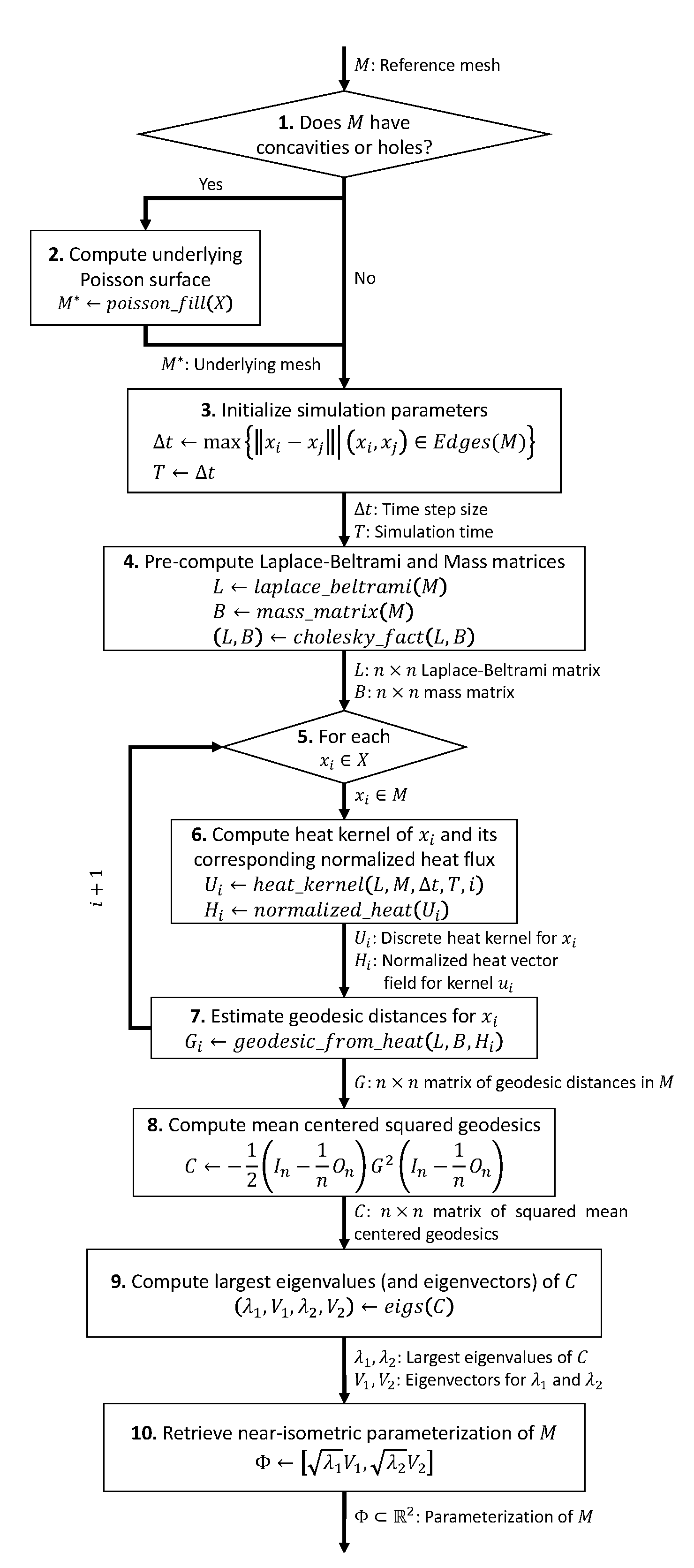
2.2. Mesh Heat Kernels

A heat kernel of a point $x_i\in M$ is a function $u_i:M\times (0,T]\to \mathbb{R}$ that satisfies the following partial differential equation [27]:

$$\begin{array}{cc}\hfill \frac{\partial u_i(x,t)}{\partial t}+\Delta u_i(x,t)& =0,x\in M,t\in (0,T],\hfill \\ \hfill {\left.\frac{\partial u(x,t)}{\partial n}\right|}_{\partial M}& =0,\hfill \\ \hfill u_i(x,0)& ={\delta }_{x_i}\left(x\right),\hfill \end{array}$$

(2)

where $\Delta$ is the Laplace–Beltrami operator, $u_i$ is the temperature distribution (heat kernel) associated to the source point $x_i$, $x\in M,t\in (0,T]$ are the spatial and time coordinates, respectively, and $T>0$ is the simulation time. The term ${\left.\frac{\partial u(x,t)}{\partial n}\right|}_{\partial M}=0$ corresponds to the Neumann boundary condition (no boundary heat flux). Finally, the term $u_i(x,0)={\delta }_{x_i}\left(x\right)$ corresponds to Dirac delta initial conditions, i.e.,

$$\begin{array}{cc}\hfill {\delta }_{x_i}\left(x\right)& =\left\{\begin{array}{cc}\infty \hfill & \mathrm{if}x=x_i,\hfill \\ 0\hfill & \mathrm{otherwise}\hfill \end{array}\right.\hfill \\ \hfill {\int }_M{\delta }_{x_i}& =1.\hfill \end{array}$$

(3)

The above initial conditions dictate initial infinite temperature at vertex $x_i$ and 0 everywhere else. After some timem $t>0$ has passed, heat dissipates from $x_i$ as illustrated in Figure 2.

Equation (2) can be solved using a Finite Element discretization scheme, as follows:

$$(\Delta tL+B)U_i^{(t+\Delta t)}=B{U}_i^{\left(t\right)},$$

(4)

where $\Delta t$ is the time step, $U_i^{\left(t\right)}=\{u_{i1}^{\left(t\right)},u_{i2}^{\left(t\right)},\cdots ,u_{in}^{\left(t\right)}\}$ is the vector of temperatures values ($u_{ij}^{\left(t\right)}=u_i(x_j,t)$), and L and B are the $n\times n$ Laplace–Beltrami and mass (sparse and symmetric) matrices, respectively. For a given edge $e_{ij}=(x_i,x_j)$, the Laplace–Beltrami matrix L is defined as follows:

$$L_{ij}=\left\{\begin{array}{cc}\frac{cot{\alpha }_{ij}+cot{\beta }_{ij}}{2},\hfill & e_{ij}\in Edges\left(M\right)\hfill \\ -\sum _{k\in E_i^{*}}{L}_{ik},\hfill & i=j\hfill \\ 0,\hfill & \mathrm{otherwise}\hfill \end{array}\right.$$

(5)

where ${\alpha }_{ij},{\beta }_{ij}\in (0,\pi )$ are the two opposite angles to the edge $e_{ij}$, and $S_i^{*}=\left\{k\right|e_{ik}\in Edges\left(M\right)\}$ is the index set of all incident edges to the vertex $x_i\in X$. The entries $L_{ij}$ of the matrix L are known as cotangent weights [28].

Similarly, the mass matrix B is defined as follows:

$$B_{ij}=\left\{\begin{array}{cc}\frac{|t_1|+|t_2|}{12},\hfill & t_1,t_2\in \mathcal{T}\mathrm{adjacent}\mathrm{triangles}\mathrm{to}{e}_{ij}\in Edges\left(M\right)\hfill \\ \sum _{k\in S_i^{*}}{B}_{ik},\hfill & i=j\hfill \\ 0,\hfill & \mathrm{otherwise},\hfill \end{array}\right.$$

(6)

where $t_1,t_2\in \mathcal{T}$ are the pair of triangles adjacent to the edge $e_{ij}$ and $|t_l|$ is the area of the triangle $t_l$ ($l=1,2$).

For each vertex $x_i\in M$, Equation (4) is solved for $U_i$ using a sparse Cholesky linear solver. It is worth noting that for every $x_i$ and $t\in (0,T]$, the matrices $\Delta tL$ and B are the same. As a consequence, these matrices are prefactored only once using Cholesky factorization, which speeds up the computation of the heat kernels.

Finally, the simulation parameters $\Delta t,T$ are chosen according to [23]:

$$\begin{array}{cc}\hfill \Delta t& =\left\{\left.\parallel x_i-x_j\parallel \right|(x_i,x_j)\in Edges\left(M\right)\right\},\hfill \\ \hfill T& =\Delta t,\hfill \end{array}$$

(7)

with $\Delta t$ computed as the magnitude of the largest edge in M, and T is equal to $\Delta t$. These values have provided better results in our parameterization experiments than other values.

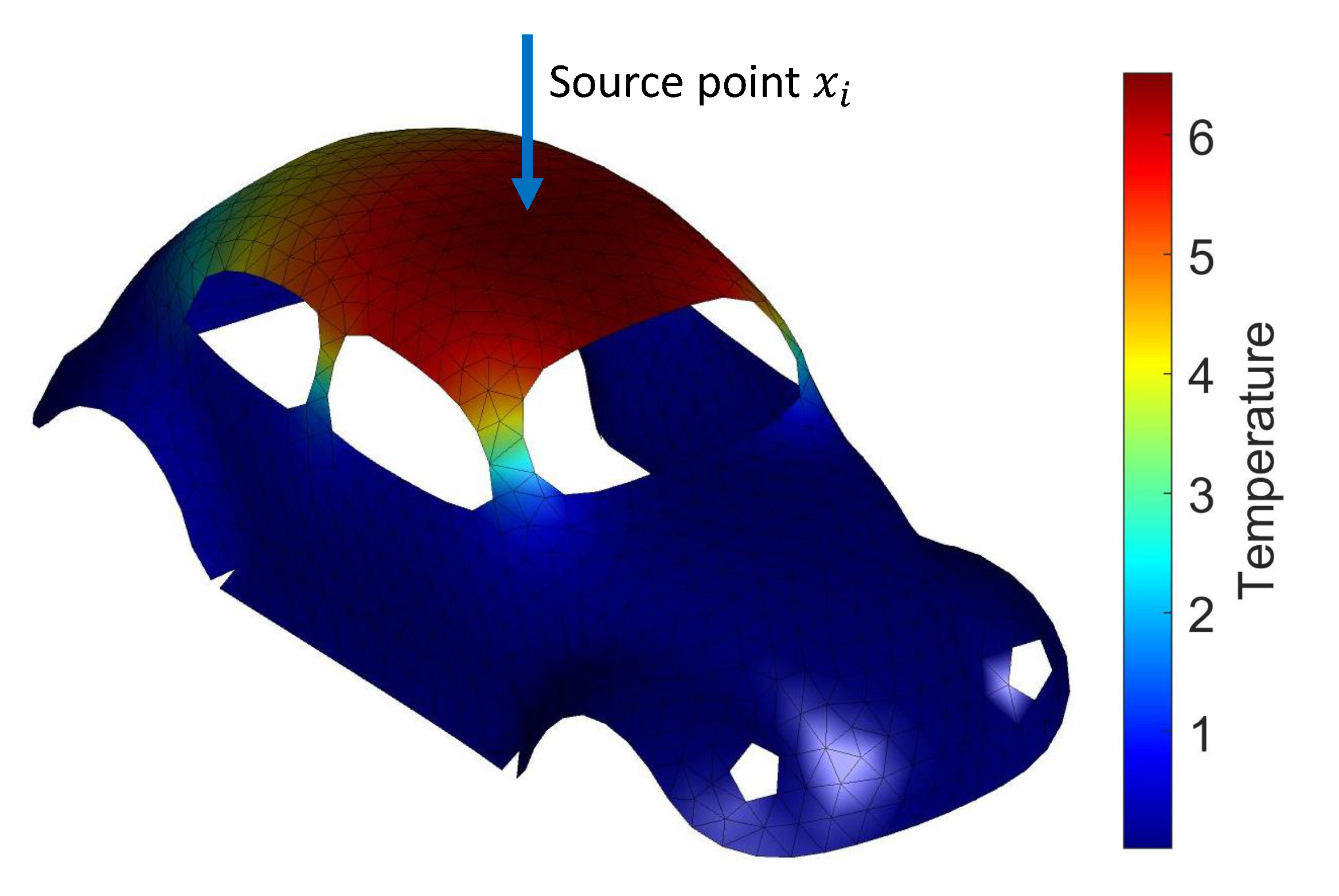
2.3. Heat-Based Geodesic Distance

The vector field $-\nabla u_i(x,t)$ (∇: gradient operator on M) describes the heat flux on M for the respective heat kernel $u_i$. The normalized heat flux vector field $H_i$ is defined as follows:

$${\overrightarrow{H}}_i(x,t)=-\frac{\nabla u_i(x,t)}{\parallel \nabla u_i(x,t)\parallel }.$$

(8)

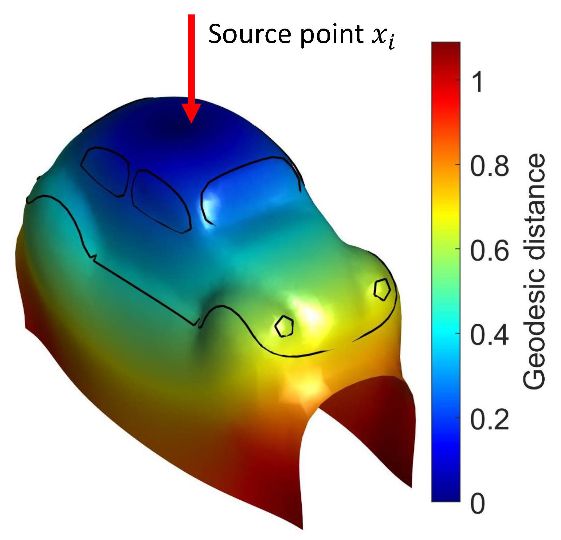
It is worth noting that the magnitude of the vector field ${\overrightarrow{H}}_i$ is 1 everywhere ($\parallel {\overrightarrow{H}}_i(x,t)\parallel =1$). In addition, as illustrated in Figure 3, the temperature contours are perpendicular to the geodesic paths from $x_i\in M$, and the corresponding vector field points in the same direction as such paths.

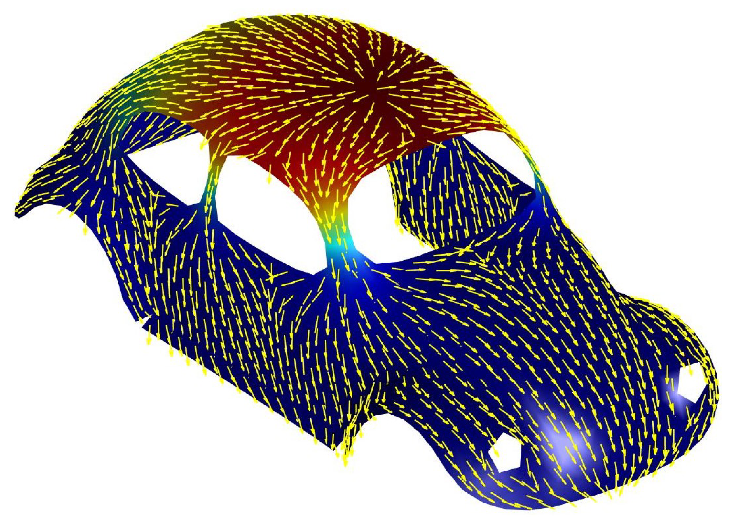
The geodesic field $g(x_i,x_j)$ satisfies the following differential equation [23]:

$$\Delta g(x_i,x)=\underset{T\to 0}{lim}\nabla ·{\overrightarrow{H}}_i(x,T),$$

(9)

where $\nabla ·{\overrightarrow{H}}_i(x,T)$ is the divergence field of the normalized heat flux. Similar to Equation (2), Equation (9) is discretized using the same Finite Element scheme, as follows:

$$L{G}_i=\underset{T\to 0}{lim}B{K}_i^{\left(T\right)},$$

(10)

where $G_i=\{g_{i1},g_{i2},\cdots ,g_{in}\}$ is the vector of geodesic distances $g_{ij}=g(x_i,x_j)$ and $K_i^{\left(T\right)}=\{k_{i1}^{\left(T\right)},k_{i2}^{\left(T\right)},\cdots ,k_{in}^{\left(T\right)}\}$ is the divergence field of the normalized gradient $k_{ij}^{\left(T\right)}=\nabla ·{\overrightarrow{H}}_i(x_j,T)$ [23]. Figure 4 plots the estimated geodesic distance field $g(x_i,x)$ for the vertex $x_i$.

2.4. Multidimensional Scaling (MDS)

After the geodesic field $g_{ij}=g(x_i,x_j)$ has been estimated on M, the minimization problem in Equation (1) can be solved. Classic multidimensional scaling poses an equivalent minimization problem [29]:

$$\underset{\mathsf{\Phi }}{min}\sum _{ij}{\left[\frac{1}{n}\left(\sum _{kl}{g}_{kl}^2\right)-g_{ij}^2-2{\varphi }_i·{\varphi }_j\right]}^2.$$

(11)

Let C be the symmetric, semidefinite positive matrix whose entries contain the mean centered squared geodesics (i.e., $C_{ij}=-\frac{1}{2}[g_{ij}^2-\frac{1}{n}\left({\sum }_{kl}{g}_{kl}^2\right)]$). In matrix form, C is equivalent to

$$C=-\frac{1}{2}\left(I_n-\frac{1}{n}{J}_n\right)G^2\left(I_n-\frac{1}{n}{J}_n\right),$$

(12)

where $I_n$, $J_n$ are the $n\times n$ identity and all-ones matrices, respectively, and $G^2$ is the $n\times n$ symmetric matrix whose entries contain the squared geodesic distances in M, i.e., $G_{ij}^2=g_{ij}^2$. Then, Equation (11) becomes:

$$\underset{\mathsf{\Phi }}{min}{\parallel C-\mathsf{\Phi }{\mathsf{\Phi }}^T\parallel }_F^2$$

(13)

with ${\parallel A\parallel }_F^2={\sum }_{ij}{A}_{ij}^2$ as the (squared) Frobenius norm of A.

Finally, Equation (13) can be solved by an eigendecomposition of C as follows [29]. Let ${\lambda }_1$ and ${\lambda }_2$ be the largest positive eigenvalues of C, with respective $n\times 1$ eigenvectors $V_1$ and $V_2$. The near-isometric parameterization of M becomes

$$\mathsf{\Phi }=[\sqrt{{\lambda }_1}{V}_1,\sqrt{{\lambda }_2}{V}_2],$$

(14)

where $\sqrt{{\lambda }_1}{V}_1$ are the discrete u-coordinates and $\sqrt{{\lambda }_2}{V}_2$ are the discrete v-coordinates of the parameterization $\mathsf{\Phi }=\{{\varphi }_1,{\varphi }_2,\dots ,{\varphi }_n\}\subset {\mathbb{R}}^2$. Figure 5 plots the resulting parameterization using MDS on the estimated geodesic fields G.

2.5. Poisson Mesh Reconstruction

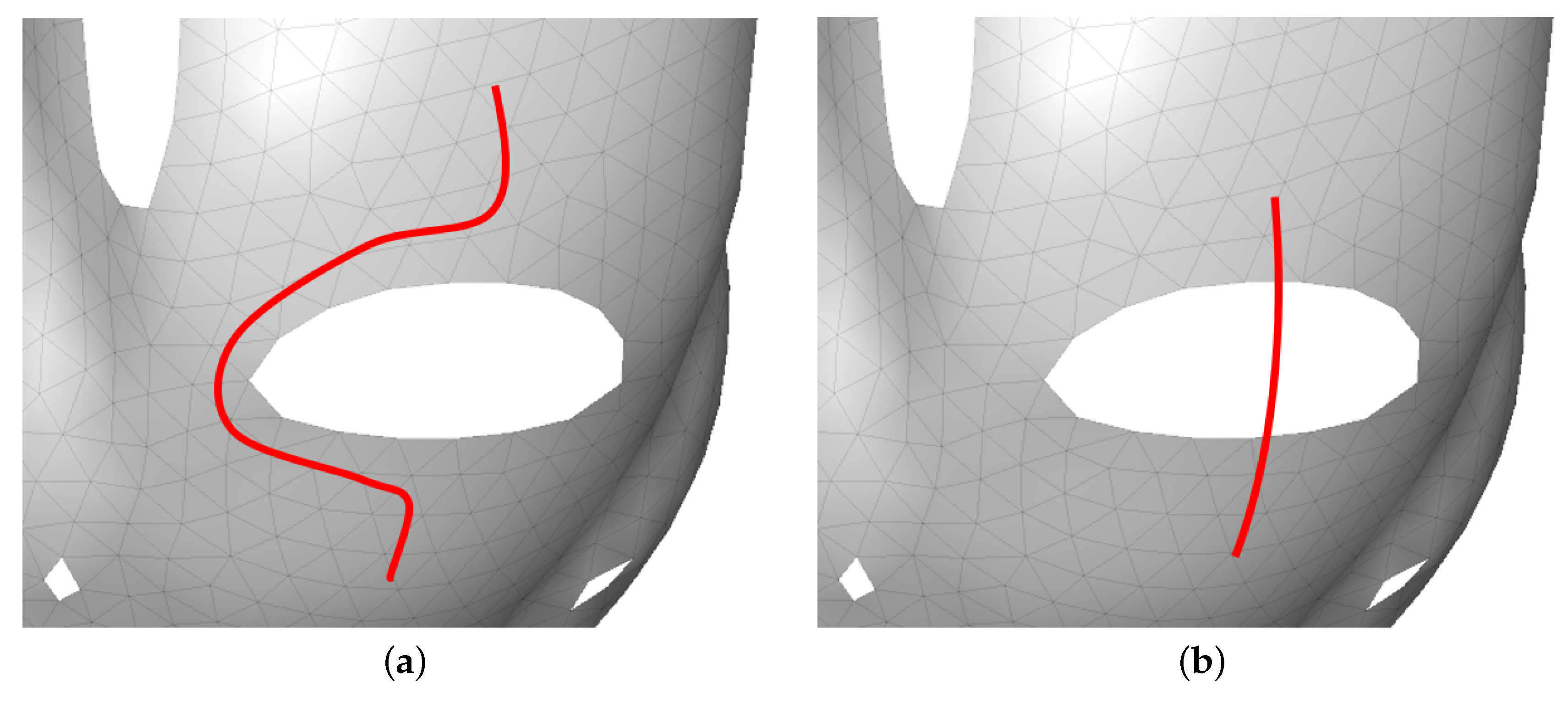
In the case that M is nonconvex (i.e., it has holes or concavities), we seek to compute an underlying extending surface $M^{*}$. Such a surface contains the points in M, and fills the holes and concavities by extending M in such areas ($M\subset M^{*}$). As an example, a geodesic path in a nonconvex M circles a given hole (Figure 6a). On the other hand, the same geodesic path in the extended surface $M^{*}$ crosses through the hole (Figure 6b).

To compute the surface $M^{*}$, our parameterization algorithm uses Poisson surface reconstruction [22] from the PCL library [25]. Define $\chi :{\mathbb{R}}^3\to \mathbb{R}$ as an indicator function such that $\chi \left(x\right)=1$ if $x\in {\mathbb{R}}^3$ is “inside” the solid defined by $M^{*}$; and $\chi \left(x\right)=0$ if x is “outside” such solid. The surface $M^{*}$ is composed by the points in between, as follows [22]:

$$M^{*}=\left\{\left.p\in {\mathbb{R}}^3\right|\chi \left(p\right)=\frac{1}{n}\sum _{x\in M}\chi \left(x\right)\right\}.$$

(15)

The indicator function $\chi$ is computed by solving the following partial differential equation in ${\mathbb{R}}^3$ [22]:

$$\Delta \chi \left(x\right)=\nabla ·\overrightarrow{N}\left(x\right),$$

(16)

where $\Delta$ and ∇ are the ${\mathbb{R}}^3$ Euclidean Laplacian and gradient operators, respectively. It is worth noting that these Laplacian and gradient operators are different from the 2-manifold version presented in Section 2.2 and Section 2.3. $\overrightarrow{N}:{\mathbb{R}}^3\to {\mathbb{R}}^3$ is a vector field in ${\mathbb{R}}^3$ whose value $\overrightarrow{N}\left(x\right)$ is the normal vector to the original surface M if $x\in M$, and $\overrightarrow{N}\left(x\right)=0$ everywhere else.

To solve Equation (16), the PCL library uses a hierarchical 3D spatial discretization and a Finite Differences approach [25].

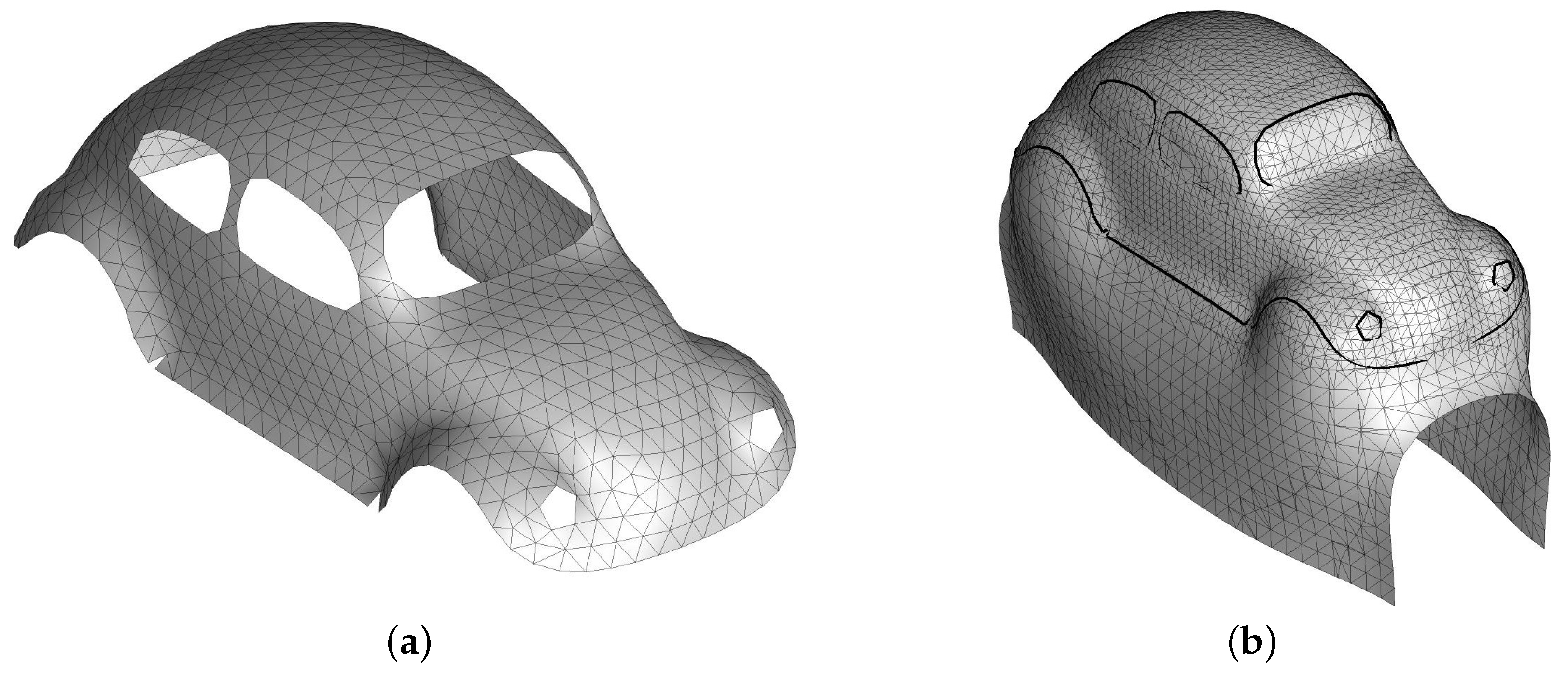
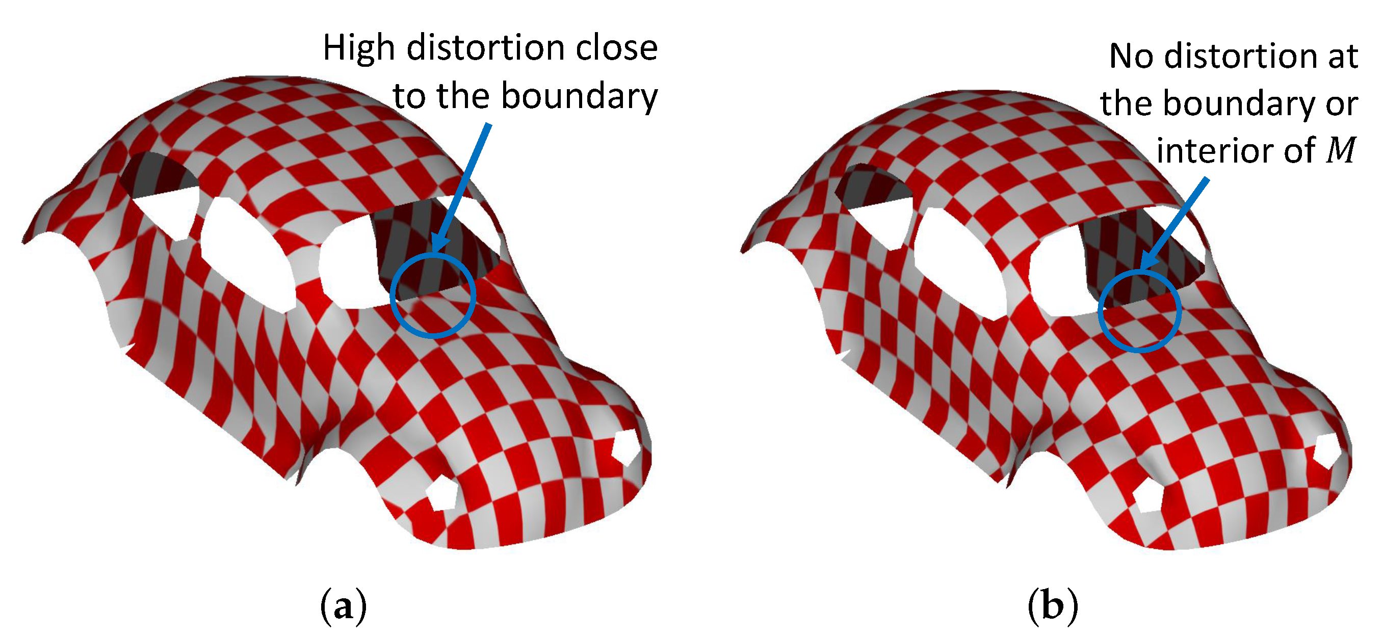
Figure 7 plots the Poisson surface filling $M^{*}$ for a given nonconvex mesh M. The resulting geodesic field (Figure 8) is distributed along the original mesh M and its extents $M^{*}-M$. The corresponding parameterization of the underlying Poisson surface $M^{*}$ (Figure 9a) is finally trimmed in order to retrieve the final parameterization $\mathsf{\Phi }$ of M (Figure 9b). Figure 10 plots the chessboard texture maps for both parameterization without Poisson filling (Figure 10a) and parameterization with Poisson surface filling (Figure 10b). As illustrated, using Poisson filling reduces parameterization distortions close to mesh holes and boundary concavities.

3. Results

To test our mesh parameterization algorithm, we run tests with several parameterizable surfaces. Section 3.1 presents a comparison of our mesh parameterization algorithm without Poisson surface filling vs. Poisson surface filling, for quasi-developable nonconvex meshes. Section 3.2 presents parameterization results for some challenging, strongly nondevelopable data sets. Finally, Section 3.3 presents the application of our parameterization algorithm for the reverse engineering of a scanned cow vertebra.

3.1. Nonfilling vs. Poisson Filling Parameterization

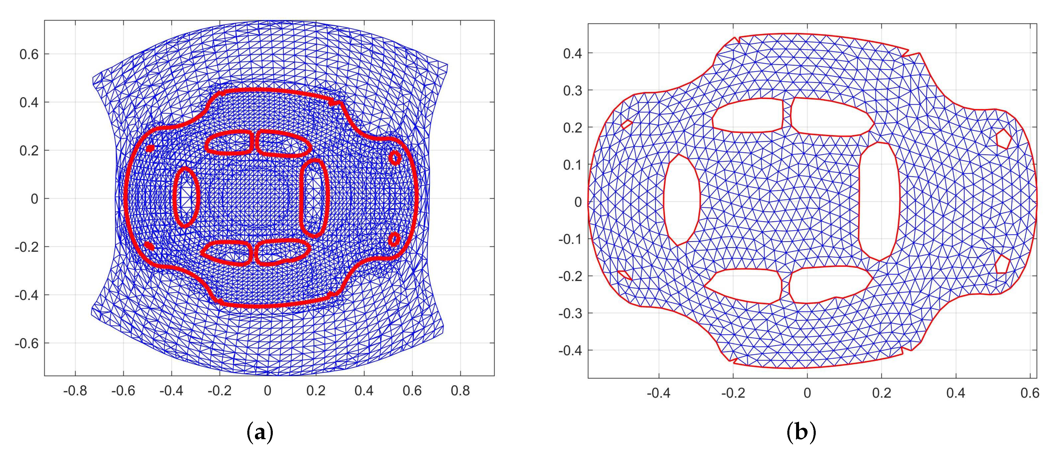
Figure 11 plots the parameterization results (2D $\mathsf{\Phi }$ coordinates and 3D texture map) for the Mask data set. Without using Poisson surface reconstruction, the resulting parameterization is bijective with relatively low distortion, except for the eye holes (Figure 11a). However, such a parameterization is improved by applying the Poisson reconstruction, reducing the distortion close to mesh holes and boundary concavities (Figure 11b).

A more extreme case is illustrated in Figure 12, with the S-trimmed-on-cone data set from [14]. Since the S shape is trimmed on a cone, M is a fully developable surface. Yet, the heat-geodesic parameterization on M fails to compute a bijective parameterization (Figure 12a). Application of Poisson (extended underlying surface $M^{*}$) filling (Figure 12b) solves this issue, resulting in a nondistorted bijective parameterization. This case illustrates (a) the vulnerability of geodesic-based parameterizations in the presence of mesh holes or concavities at mesh borders, (b) the capacity of the underlying Poisson extended surface to prevent (a), (c) the natural manner in which geodesic curves isometrically parameterize a developable surface.

3.2. Parameterization of Strongly Nondevelopable Meshes

In this section, the public data sets Foot, Gargoyle, and Cow are parameterized with our heat-based geodesics algorithm. These benchmark datasets contain an artificially introduced border [30], which allows their parameterization. Figure 13a,b plot the parameterization results for the seam Foot and Gargoyle, respectively. The resulting parameterization is bijective, with some noticeable distortion (e.g., in the Gargoyle head). 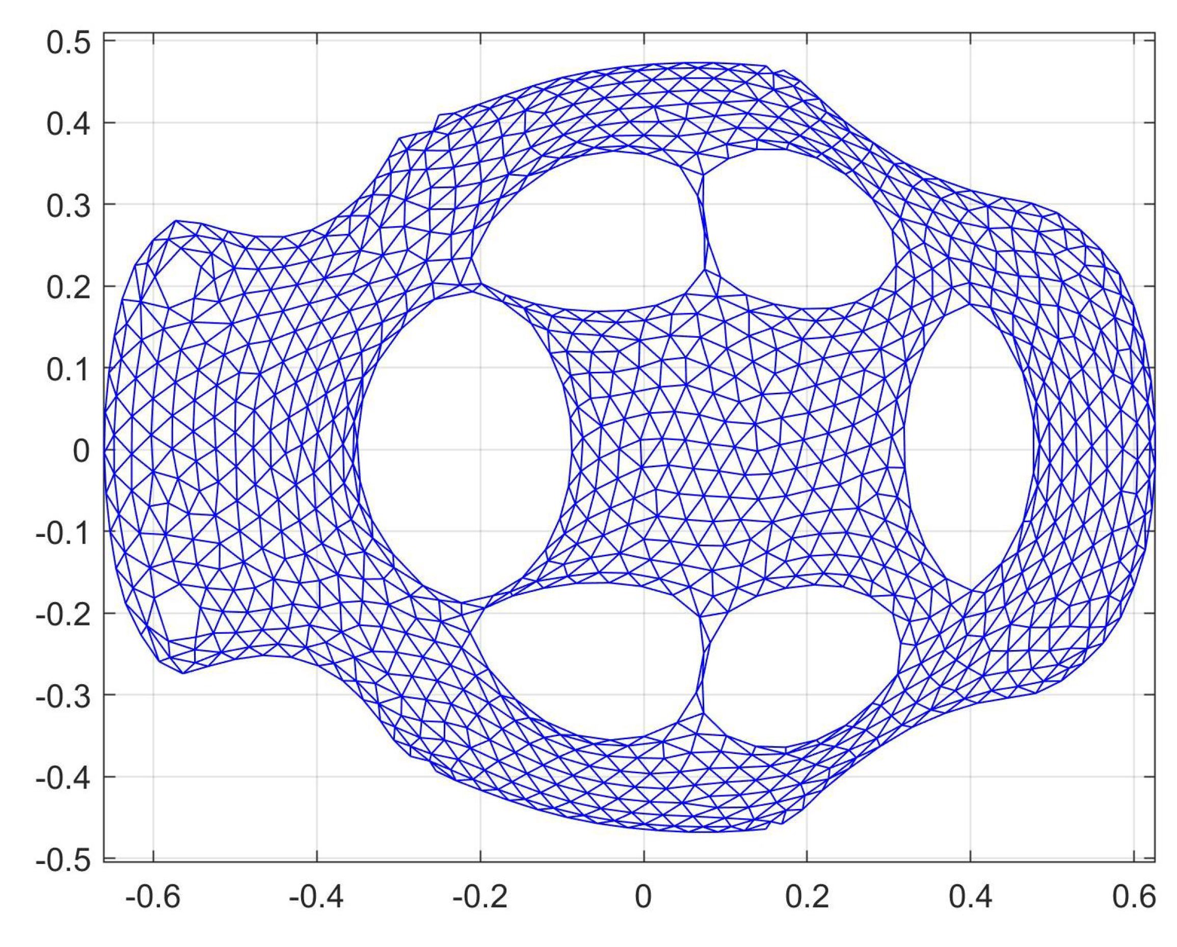Figure 13c plots our parameterization results for the seamed Cow, which is not bijective in the head, legs, and tail.

It is worth noting that although parameterizable, these benchmark data sets are strongly nondevelopable without a proper mesh presegmentation. This fact is illustrated in the next section.

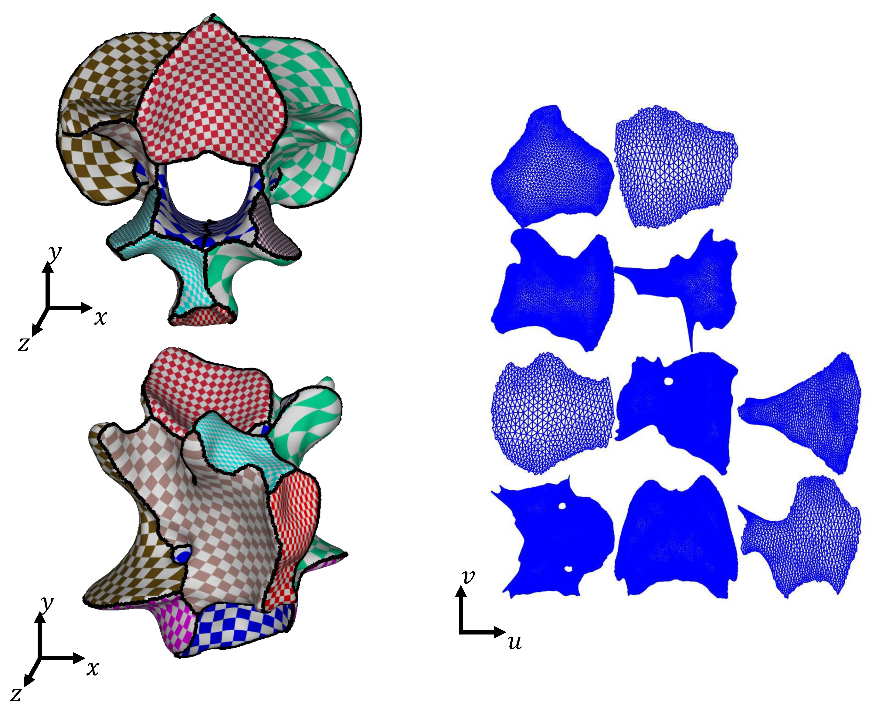
3.3. Reverse Engineering of Cow Vertebra

For this section, the vertebra of a cow is scanned using a 3D optical scanner. The scanned mesh is closed and therefore accepts no (bijective) parameterization. The closed mesh is segmented into quasi-developable meshes using a heat-based segmentation approach [31]. Figure 14 plots the parameterization results for the segmented mesh. Each submesh bijective parameterization presents low distortion, enabling further reverse engineering operations such as NURBs reparameterization [14], finite element analysis, structural optimization, and/or dimensional inspection [31].

4. Conclusions

This article presents the implementation of a novel application of heat propagation in 2-manifolds used for mesh parameterization. The temperature contours for the heat kernels computed on the mesh are perpendicular at each point to the geodesic curves in the surface. This principle permits determination of geodesic maps in the mesh and in particular vertex-to-vertex geodesic distances. Although Finite Element methods produce better results as the mesh resolution increases (higher polygon count), the geodesics estimation method still produces robust results for low polygon count meshes as each geodesic path traverses across the mesh faces (contrary to graph algorithms which traverse the mesh graph). A quasi-isometric bijective function (i.e., the parameterization) is synthesized to map the 3D mesh to the parameter (2D) space. This parameterization is near isometric in the sense that geodesic distance on the mesh between any two points on the mesh approximates the Euclidean distance between their images in the parametric space. This approach is obviously limited to meshes that are quasi-developable or developable, since mesh developability is necessary for the existence of an isometric parameterization for it.

Our approach circumvents the weakness of geodesic maps in the presence of mesh interruptions (boundary concavities and mesh holes) by devising an underlying continuous Poisson surface that approximates the input mesh but contains no such interruptions. This underlying surface allows for geodesic maps to be computed on it, which are also valid in the input mesh. In this manner, the parameterization computed for the Poisson surface is valid for the input mesh. Finally, the boundaries of the input mesh are explicitly marked on the parameterization to obtain a trimmed surface or FACE in the Boundary Representation jargon.

Future work is required in these aspects—(a) to eliminate redundant computation that is present in the construction of heat-based geodesic maps and (b) to use failures in the bijectiveness of the computed parameterizations to force mesh segmentation, when the input mesh is strongly nondevelopable.