Article

Three-Dimensional Hydro-Magnetic Flow Arising in a Long Porous Slider and a Circular Porous Slider with Velocity Slip

1
International Cultural Exchange School (ICES), Donghua University, West Yan’an Road 1882, Shanghai 200051, China
2
Department of Mathematics, University of Hafr Al-Batin, Hafr Al-Batin 31991, Saudi Arabia
3
Glorious Sun School of Business and Management, Donghua University, West Yan’an Road 1882, Shanghai 200051, China
4
Faculty of Science, Jiangsu University, Zhenjiang 212013, China
5
Department of Mathematics, COMSATS University Islamabad, Abbottabad 22060, Pakistan
*
Authors to whom correspondence should be addressed.
Mathematics 2019, 7(8), 748; https://doi.org/10.3390/math7080748
Submission received: 21 July 2019 / Revised: 10 August 2019 / Accepted: 12 August 2019 / Published: 16 August 2019
(This article belongs to the Special Issue Computational Fluid Dynamics 2020)

Abstract

:
The current research explores the injection of a viscous fluid through a moving flat plate with a transverse uniform magneto-hydrodynamic (MHD) flow field to reduce sliding drag. Two cases of velocity slip between the slider and the ground are studied: a long slider and a circular slider. Solving the porous slider problem is applicable to fluid-cushioned porous sliders, which are useful in reducing the frictional resistance of moving bodies. By using a similarity transformation, three dimensional Navier–Stokes equations are converted into coupled nonlinear ordinary differential equations. The resulting nonlinear boundary value problem was solved analytically using the homotopy analysis method (HAM). The HAM provided a fast convergent series solution, showing that this method is efficient, accurate, and has many advantages over the other existing methods. Solutions were obtained for the different values of Reynolds numbers (R), velocity slip, and magnetic fields. It was found that surface slip and Reynolds number had substantial influence on the lift and drag of the long and the circular sliders. Moreover, the effects of the applied magnetic field on the velocity components, load-carrying capacity, and friction force are discussed in detail with the aid of graphs and tables.

1. Introduction

It is a well-established fact that a moving body reduces drag if it is elevated by a layer of air. This phenomenon is used in air-cushioned vehicles and in air hockey, in which the frictional resistance of moving objects is reduced. Skalak and Wang [1] were the pioneers of studying the three-dimensional flow that arises between a moving porous flat plate and the ground, and they later on wrote an erratum on their own paper [2]. Wang also studied elliptical porous sliders [3]. In the case of Newtonian fluids, past studies have included porous circular, long, inclined, and elliptical sliders. R. C. Bhattacharjee studied a porous slider bearing lubricated with a coupled stress (a magneto-hydrodynamic (MHD) fluid) [4]. Jimit made a comparison of the different porous structures on the performance of a magnetic fluid [5]. Prawal Sinha analyzed the thermal effects of a long porous rough slider bearing [6]. Mohmmadrayian analyzed a rough porous inclined slider bearing lubricated with a ferrofluid in consideration of slip velocity [7]. Ji Lang both theoretically and experimentally investigated the transient squeezing flow in a highly porous film [8]. Similarly, a large amount of literature is available in relation to long porous sliders (LPSs) [1,6,9,10,11,12,13] and circular porous sliders (CPSs) [2,14,15,16,17,18]. Awati investigated the lubrication of a long porous slider by using the homotopy analysis method (HAM) [10]. In a separate study, Khan studied the effects of Reynolds numbers by using different analytical methods [11,12]. Naeem studied the influence of Reynolds numbers (R) on long [13] and circular porous sliders [18]. Ghoreishi studied the circular slider [14]. Madani investigated the circular porous slider by using HPM, and also analyzed its lift and drag [19].
All the above mentioned studies were done without a slip condition on either the immobile ground or slider. However, a slip condition is essential for super-hydrophobic planes, as it is difficult to have a zero mean tangential velocity from where the fluid is injected when there is a slip. Furthermore, in order to minimize adhesion, the fluid could be a rarefied gas, where the compact exterior could be coated with a material, or the ground could be uneven so that an equivalent slip exists or there is a slip flow regime. Wang [16] discussed slip effects, but didn’t consider the effects of a transverse magnetic field. Therefore, the goal of the current work is to examine the impact of slip and Reynolds numbers when a transverse magnetic field is affecting the performance of a porous slider. Through the literature survey, it is assumed that a three-dimensional flow with slip and a uniform magnetic field does not exist. Hence, the goal of the current research is to analyze the performance of porous sliders in the presence of slip and a Reynolds number with a constant magnetic field, and to assess their effects on the components of velocity lift and drag.
The structure of the article is as follows: In the introduction, a brief history of the problem of the porous slider and its application is presented. In the second section, the formulation of the problems are given, while in the third section the formulation of a homotopic solution is presented [20]. The fourth section deals with the convergence criteria of the HAM. Results and discussions are given in the fifth section. Finally, the conclusion is given in the sixth section, with a list of nomenclature.
As discussed above, the velocity slip condition is considered in this study. Navier introduced the slip condition for the first time as follows:
x 1 = H ς
In Equation (1), tangential velocity u is proportional to the shear stress and H is the constant of proportionality, which is actually a slip coefficient. In order to ignore the end effects, it is assumed that the gap between slider and ground is quite small as compared to the slider’s lateral dimension. Both circular and long porous sliders are considered in this study.

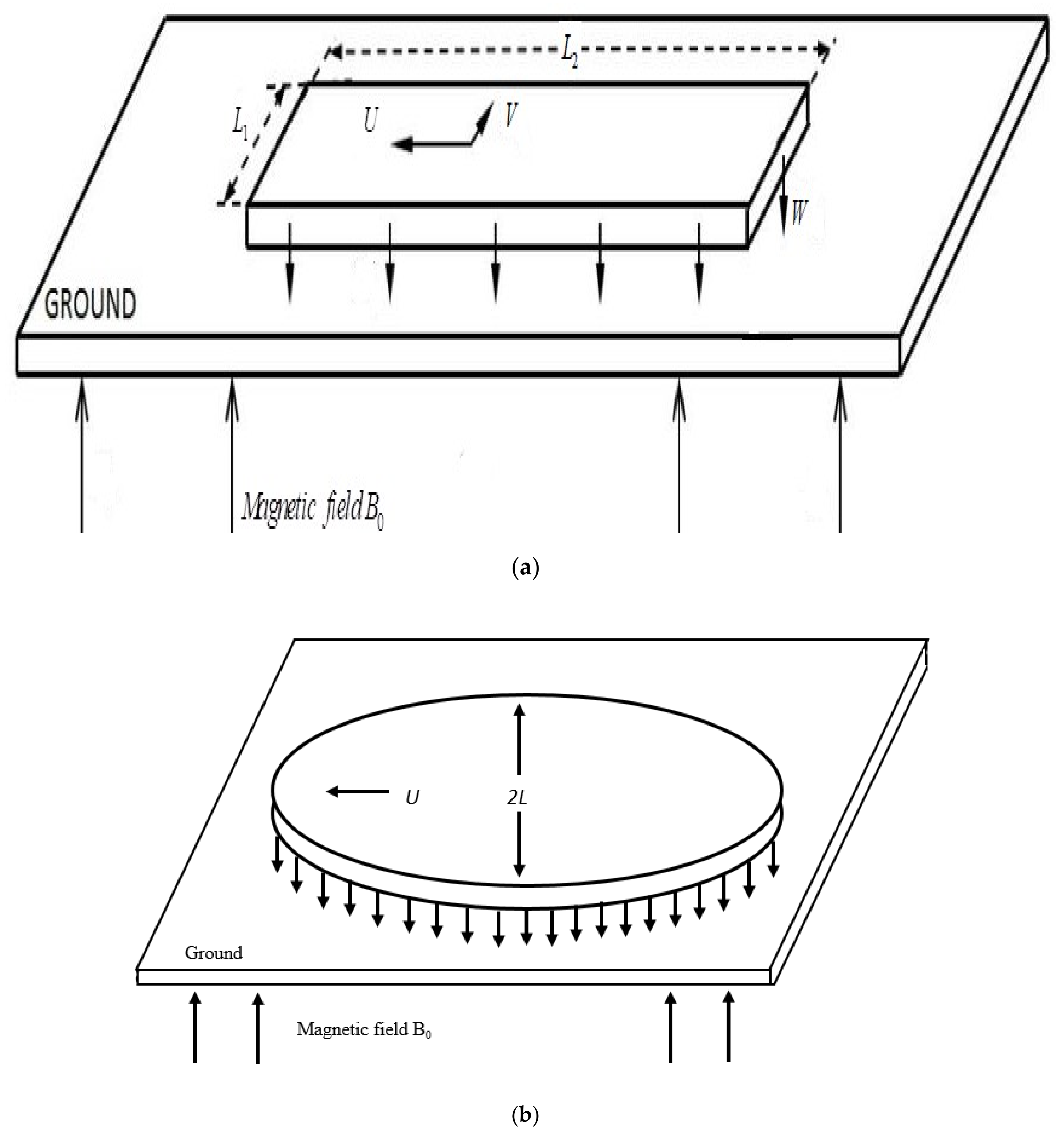
2. Problem Formulation of Long and Circular Sliders

In this study, the incompressible and steady flow of a viscous fluid between porous (long and circular) sliders and the ground is considered in the presence of a uniform magnetic field, as shown in Figure 1.
Length and width are quite big compared to height d . The slider moves with the velocity components and is elevated because of the injection of fluid from below with a magnetic field applied externally. In order to avoid the induced magnetic field formed by the movement of the fluid, it is assumed that the magnetic Reynolds number is not very big. Furthermore, the induced and imposed electric field are supposed to be negligible, and therefore the electromagnetic body force per unit volume simplifies F e m = σ 0 ( v × B ) × B , where B = ( 0 , 0 , B 0 ) is the magnetic field.
Under the above-stated assumptions and conditions, Navier–Stokes equations take the following form:
ϕ 1 ϕ 1 x 1 + ϕ 2 ϕ 1 x 2 + ϕ 3 ϕ 1 x 3 = 1 ρ p x 1 + υ ( 2 ϕ 1 x 1 2 + 2 ϕ 1 x 2 2 + 2 ϕ 1 x 3 2 ) σ 0 ρ B 0 2 ϕ 1
ϕ 1 ϕ 2 x 1 + ϕ 2 ϕ 2 x 2 + ϕ 3 ϕ 2 x 3 = 1 ρ p x 2 + υ ( 2 ϕ 2 x 1 2 + 2 ϕ 2 x 2 2 + 2 ϕ 2 x 3 2 ) σ 0 ρ B 0 2 ϕ 2
ϕ 1 ϕ 3 x 1 + ϕ 2 ϕ 3 x 2 + ϕ 3 ϕ 3 x 3 = 1 ρ p x 3 + υ ( 2 ϕ 3 x 1 2 + 2 ϕ 3 x 2 2 + 2 ϕ 3 x 3 2 )
Velocity components are expressed as ( ϕ 1 , ϕ 2 , ϕ 3 ) , where ρ , p , and υ are density, pressure and kinematic viscosity, respectively. Law of conservation of mass is as follows:
ϕ 1 x 1 + ϕ 2 x 2 + ϕ 3 x 3 = 0
According to Naeem [13], the following transform has been used:
ϕ 1 = U ψ 1 ( ς ) + W d x 1 ψ 3 / ( ς ) , ϕ 2 = V ψ 2 ( ς ) , ϕ 3 = W ψ 3 ( ς ) .
where ς = x 3 d . By adding Equation (6) into Equations (2)–(4), the following ordinary differential equations are obtained:
ψ 3 i v = R ( ψ 3 / ψ 3 / / ψ 3 ψ 3 / / / ) + M 2 ψ 3 /
ψ 1 / / = R ( ψ 1 ψ 3 / ψ 3 ψ 1 / ) + M 2 ψ 1
ψ 2 / / = R ( ψ 1 ψ 2 / ) + M 2 ψ 2
where R is the Reynolds number ( R = W d / υ ). Boundary conditions at x 3 = 0 and x 3 = d are given in Equations (10) and (11), respectively.
ϕ 1 = U + H 1 μ ϕ 1 x 3 , ϕ 2 = V + H 1 μ ϕ 2 x 3 , ϕ 3 = 0
ϕ 1 = H 2 μ ϕ 1 x 3 , ϕ 2 = H 2 μ ϕ 2 x 3 = 0 , ϕ 3 = W
where H 1 ,   H 2 , and μ = ρ υ are slip coefficients and viscosity, respectively. Equations (10) and (11) take the following form:
ψ 3 / ( 0 ) = β 1 ψ 3 / / ( 0 ) = , ψ 3 ( 0 ) = 0 , ψ 3 ( 1 ) = 1 , ψ 3 / ( 1 ) = β 2 ψ 3 / / ( 1 ) , ψ 1 ( 1 ) = β 2 ψ 1 / ( 1 ) , ψ 1 ( 0 ) 1 = β 1 ψ 1 / ( 0 ) , ψ 2 ( 1 ) = β 2 ψ 2 / ( 1 ) , ψ 2 ( 0 ) 1 = β 1 ψ 2 / ( 0 ) .
where β 1 = H 1 μ / d , β 2 = H 2 μ / d are slip factors. Equations (7)–(9) and (12) will be solved by the HAM. The expression for pressure can be deduced from Equations (2)–(4) as follows:
p ρ = W 2 Λ x 1 2 2 d + 1 2 ϕ 3 2 γ ϕ 3 , x 3 + A
where Λ , A are constants and
Λ = ( ψ 3 / ) 2 ψ 3 ψ 3 / / 1 R ψ 3 / / / = ( ψ 3 / ( 0 ) ) 2 1 R ψ 3 / / / ( 0 ) .
If 2 l is the width of the slider with ambient pressure ρ 0 , then Equation (13) gives
p p 0 = ρ Λ W 2 ( x 1 2 l 2 ) 2 d 2 .
The relationship between depth and lift can be expressed as follows:
L = 1 1 ( p p 0 ) d x = 2 ρ W 2 l 3 3 d 2 Λ .
where 2 ρ W 2 l 3 / ( 3 d 2 ) is normalized factor. The relationship between depth and drag in the x 1 direction is
D x 1 = 1 1 μ ϕ 1 x 3 | z = d d x 1 = 2 μ U l d ψ 1 / ( 1 ) .
Similarly, 2 μ U l / d is the normalized factor of drag in the x 1 direction, which is ψ 1 / ( 1 ) , while ψ 2 / ( 1 ) is normalized drag for the x 2 direction:
D x 2 = 1 1 μ ϕ 2 x 3 | z = d d x 1 = 2 μ V l d ψ 2 / ( 1 ) .
Similarly, from Figure 1b, a circular slider can be seen, where L is the radius of the slider (which can be assumed to be comparatively bigger than the width). Since the slider is levitated, the axes on the slider can be fixed so that the ground is moving with a velocity component in the x 1 direction. For the circular slider, a similar transform [18] helps to reduce the partial differential equations into ordinary differential equations:
x 1 = U ψ 5 ( ς ) + W d x 1 ψ 4 / ( ς ) , x 2 = W d x 2 ψ 4 / ( ς ) , x 3 = 2 W ψ 4 ( ς ) .
With the help of Equation (19), Equations (2)–(4) take the following form
ψ 4 i v 2 R ψ 4 ψ 4 / / / M 2 ψ 4 / = 0
ψ 5 / / R ( ψ 5 ψ 4 / 2 ψ 4 ψ 5 / ) M 2 ψ 5 = 0
p ρ = W 2 Λ ( x 1 2 + x 2 2 ) 2 d + 1 2 x 3 2 γ x 3 , x 3 + C
in which Λ , C are constants and
Λ 1 = ( ψ 4 / ( 0 ) ) 2 1 R ψ 4 / / / ( 0 ) .
The boundary conditions on x 3 = 0 & d :
ψ 4 / ( 0 ) = β 1 ψ 4 / / ( 0 ) = , ψ 4 ( 0 ) = 0 , ψ 4 ( 1 ) = 1 / 2 , ψ 4 / ( 1 ) = β 2 ψ 4 / / ( 1 ) , ψ 5 ( 1 ) = β 2 ψ 5 / ( 1 ) , ψ 5 ( 0 ) 1 = β 1 ψ 5 / ( 0 ) .
To normalize the lift, integrating the bottom of the slider as a result of the normalized factor can be expressed as π ρ W 2 l 4 / 4 d .
L = 4 d π ρ W 2 l 4 s ( p p 0 ) d s = 1 R 3 Λ .
The relationship between depth and drag in the x 1 direction is
D x 1 = d π μ U l 2 s H x 3 x 1 d s = 1 R 3 ψ 5 / ( 1 ) .

3. Homotopic Solution Procedure

To apply HAM [20], the following initial guesses for Equations (7)–(9), (20), and (21) can be chosen as
ψ 3 , 0 ( ς ) = 2 ς 3 ( 1 + β 1 + β 2 ) + 3 ς ( 1 + 2 β 2 ) ( ς + 2 β 1 ) 1 + 4 ( β 1 + β 2 ) + 12 β 1 β 2 , ψ 1 , 0 ( ς ) = 1 ς + β 2 1 + β 1 + β 2 , ψ 2 , 0 ( ς ) = 1 ς + β 2 1 + β 1 + β 2 , ψ 4 , 0 ( ς ) = 2 ς 3 ( 1 + β 1 + β 2 ) + 3 ς ( 1 + 2 β 2 ) ( ς + 2 β 1 ) 2 ( 1 + 4 ( β 1 + β 2 ) + 12 β 1 β 2 ) , ψ 5 , 0 ( ς ) = 1 ς + β 2 1 + β 1 + β 2
For the initial approximation, the following auxiliary linear operators can be chosen:
L ( ψ 3 ) = d 4 h d ς 4 , L ( ψ 1 ) = d 2 θ d ς 2 , L ( ψ 2 ) = d 2 θ d ς 2 , L ( ψ 4 ) = d 4 θ d ς 4 , L ( ψ 5 ) = d 2 θ d ς 2 .
which satisfies
L ψ 1 [ A 5 + A 6 ς ] = 0 , L ψ 2 [ A 7 + A 8 ς ] = 0 , L ψ 3 [ A 1 + A 2 ς + A 3 ς 2 + A 4 ς 4 ] = 0 , L ψ 4 [ A 9 + A 10 ς + A 11 ς 2 + A 12 ς 4 ] = 0 , L ψ 5 [ A 13 + A 14 ς ] = 0.
in which A i ( i = 1 14 ) are constants of integration.

Initial Order Deformation Problem

The deformation equations for the initial order can be viewed as follows:
( 1 Φ ) L ψ 1 [ ψ 1 ( ς , Φ ) ψ 1 , 0 ( ς , Φ ) ] = Φ ψ 1 H ψ 1 N ψ 1 [ ψ 1 ( ς , Φ ) ]
( 1 Φ ) L ψ 2 [ ψ 2 ( ς , Φ ) ψ 2 , 0 ( ς , Φ ) ] = Φ ψ 2 H ψ 2 N ψ 2 [ ψ 2 ( ς , Φ ) ]
( 1 Φ ) L ψ 3 [ ψ 3 ( ς , Φ ) ψ 3 , 0 ( ς , Φ ) ] = Φ ψ 3 H ψ 3 N ψ 3 [ ψ 3 ( ς , Φ ) ]
( 1 Φ ) L ψ 4 [ ψ 4 ( ς , Φ ) ψ 4 , 0 ( ς , Φ ) ] = Φ ψ 4 H ψ 4 N ψ 4 [ ψ 4 ( ς , Φ ) ]
( 1 Φ ) L ψ 5 [ ψ 5 ( ς , Φ ) ψ 5 , 0 ( ς , Φ ) ] = Φ ψ 5 H ψ 5 N ψ 5 [ ψ 5 ( ς , Φ ) ]
and the boundary conditions are
ψ 1 ( 1 , Φ ) = μ 2 ψ 1 / ( 1 , Φ ) , ψ 1 ( 0 , Φ ) 1 = μ 1 ψ 1 / ( 0 , Φ )
ψ 2 / ( 0 , Φ ) 1 = μ 1 ψ 2 / ( 0 , Φ ) , ψ 2 ( 1 , Φ ) = μ 2 ψ 2 / ( 1 , Φ )
ψ 3 / ( 0 , Φ ) = μ 1 ψ 3 / / ( 0 , Φ ) , ψ 3 ( 0 , Φ ) = 0 , ψ 3 ( 1 , Φ ) = 1 , ψ 3 / ( 1 , Φ ) = μ 2 ψ 3 / / ( 1 , Φ )
ψ 4 / ( 0 , Φ ) = μ 1 ψ 4 / / ( 0 , Φ ) , ψ 4 ( 0 , Φ ) = 0 , ψ 4 ( 1 , Φ ) = 1 / 2 , ψ 4 / ( 1 , Φ ) = μ 2 ψ 4 / / ( 1 , Φ ) ,
ψ 5 ( 1 , Φ ) = μ 2 ψ 5 / ( 1 , Φ ) , ψ 5 ( 0 , Φ ) 1 = μ 1 ψ 5 / ( 0 , Φ )
where N ψ 1 , N ψ 2 , N ψ 3 , N ψ 4 , and N ψ 5 are defined as
N ψ 3 [ ψ 3 ( ς ; Φ ) ] = ψ 3 / / / / R ( ψ 3 / ψ 3 / / ψ 3 ψ 3 / / / ) M 2 ψ 3 /
N ψ 1 [ ψ 1 ( ς ; Φ ) ] = ψ 1 / / R ( ψ 1 ψ 3 / ψ 3 ψ 1 / ) M 2 ψ 1 ,
N ψ 2 [ ψ 2 ( ς ; Φ ) ] = ψ 2 / / + R ( ψ 3 ψ 2 / ) M 2 ψ 2 ,
N ψ 4 [ ψ 4 ( ς ; Φ ) ] = ψ 4 / / / / 2 R ψ 4 ψ 4 / / / M 2 ψ 4 /
N ψ 5 [ ψ 5 ( ς ; Φ ) ] = ψ 5 / / R ( ψ 5 ψ 4 / 2 ψ 4 ψ 5 / ) M 2 ψ 5
Here, the auxiliary parameters are ψ 1 0 , ψ 2 0 , ψ 3 0 , ψ 4 0 , and ψ 5 0 , while the non-zero auxiliary functions are expressed as H ψ 1 , H ψ 2 , H ψ 3 , H ψ 4 , and H ψ 5 , and ς [ 0 , 1 ] is the embedding parameter.
From Equations (30)–(34), it is observed that when ς = 0 there is
ψ 1 ( ς , 0 ) = ψ 1 , 0 ( ς ) , ψ 2 ( ς , 0 ) = ψ 2 , 0 ( ς ) , ψ 3 ( ς , 0 ) = ψ 3 , 0 ( ς ) , ψ 4 ( ς , 0 ) = ψ 4 , 0 ( ς ) , ψ 5 ( ς , 0 ) = ψ 5 , 0 ( ς ) .
As ς = 1 and ψ 1 0 , ψ 2 0 , ψ 3 0 , ψ 4 0 , ψ 5 0 and H ψ 1 0 , H ψ 2 0 , H ψ 3 0 , H ψ 4 0 , H ψ 5 0 , then Equations (30)–(34) are obtained as
ψ 1 ( ς , 1 ) = ψ 1 ( ς ) , ψ 2 ( ς , 1 ) = ψ 2 ( ς ) , ψ 3 ( ς , 1 ) = ψ 3 ( ς ) , ψ 4 ( ς , 1 ) = ψ 4 ( ς ) , ψ 5 ( ς , 1 ) = ψ 5 ( ς ) ,
In order to get m th - order deformation equations, Equations (30)–(34) are differentiated m - times with respect to ς , after substituting ς = 0 and dividing both sides by m ! . Finally, the m th - order deformation equations take the following forms:
L ψ 1 [ ψ 1 , m ( ς ) χ m ψ 1 , m 1 ( ς ) ] = ψ 1 R 1 , m ( ς ) .
L ψ 2 [ ψ 2 , m ( ς ) χ m ψ 2 , m 1 ( ς ) ] = ψ 2 R 3 , m ( ς ) .
L ψ 3 [ ψ 3 , m ( ς ) χ ψ 3 h ψ 3 1 ( ς ) ] = ψ 3 R 3 , m ( ς ) .
L ψ 4 [ ψ 4 , m ( ς ) χ ψ 4 h ψ 4 1 ( ς ) ] = ψ 4 R 4 , m ( ς ) .
L ψ 5 [ ψ 5 , m ( ς ) χ ψ 5 h ψ 5 1 ( ς ) ] = ψ 5 R 5 , m ( ς ) .
with boundary conditions
ψ 1 , m ( 1 ) = μ 2 ψ 1 , m / ( 1 ) , ψ 1 , m ( 0 ) 1 = μ 1 ψ 1 , m / ( 0 )
ψ 2 , m ( 1 ) = μ 2 ψ 2 , m / ( 1 ) , ψ 2 , m ( 0 ) 1 = μ 1 ψ 2 , m / ( 0 )
ψ 3 , m / ( 0 ) = μ 1 ψ 3 , m / / ( 0 ) = , ψ 3 , m ( 0 ) = 0 , ψ 3 , m ( 1 ) = 0 , ψ 3 , m / ( 1 ) = μ 2 ψ 3 , m / / ( 1 )
ψ 4 , m / ( 0 ) = μ 1 ψ 4 , m / / ( 0 ) = , ψ 4 , m ( 0 ) = 0 , ψ 4 , m ( 1 ) = 0 , ψ 4 , m / ( 1 ) = μ 2 ψ 4 , m / / ( 1 )
ψ 5 , m ( 1 ) = μ 2 ψ 5 , m / ( 1 ) , ψ 5 , m ( 0 ) 1 = μ 1 ψ 5 , m / ( 0 )
where
R 1 , m ( ς ) = ψ 1 , m 1 / / R k = 0 m 1 ψ 1 , m 1 ψ 3 , k / + R k = 0 m 1 ψ 3 , m 1 ψ 1 , k /
R 2 , m ( ς ) = ψ 2 , m 1 / / + R k = 0 m 1 ψ 3 , m 1 ψ 2 , k /
R 3 , m ( ς ) = ψ 3 , m 1 / / / / R k = 0 m 1 ψ 3 , m 1 / ψ 3 , k / / + R k = 0 m 1 ψ 3 , m 1 ψ 3 , k / / /
R 4 , m ( ς ) = ψ 4 , m 1 / / / / 2 R k = 0 m 1 ψ 4 , m 1 ψ 4 , k / / / M 2 k = 0 m 1 ψ 4 , k /
R 5 , m ( ς ) = ψ 5 , m 1 / / R k = 0 m 1 ψ 5 , m 1 ψ 4 , k / 2 k = 0 m 1 ψ 4 , m 1 ψ 5 , k / / M 2 ψ 5
A well-known software called MATHEMATICA has been used to solve the modeled problem.

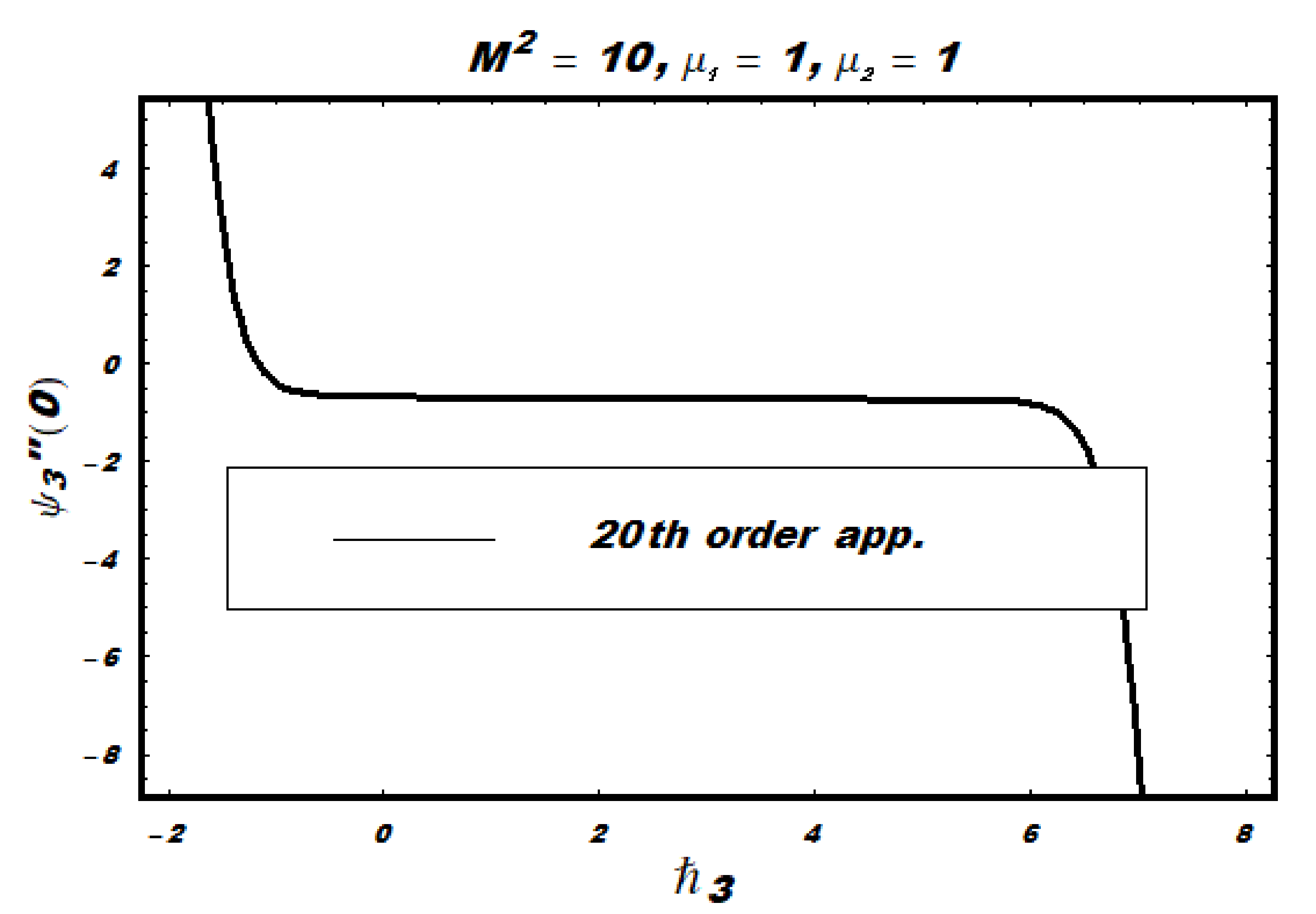
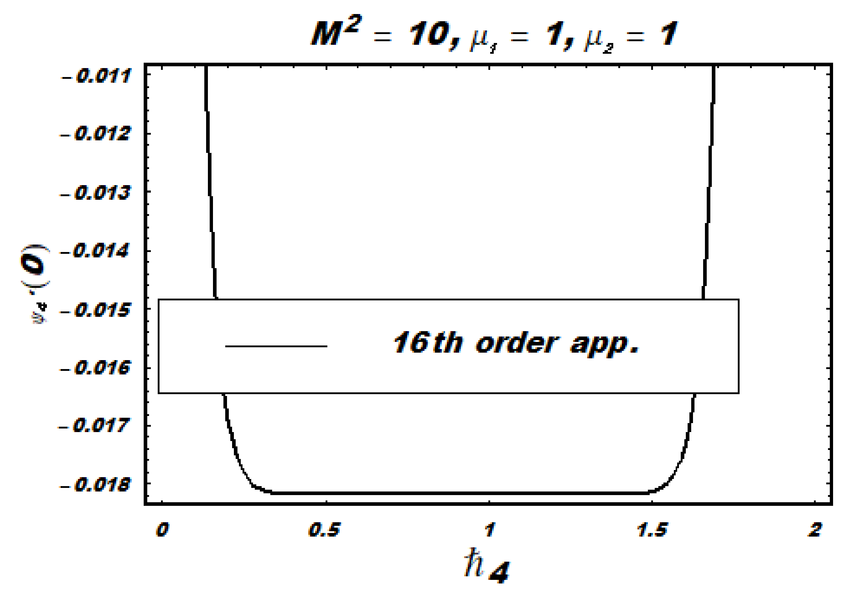
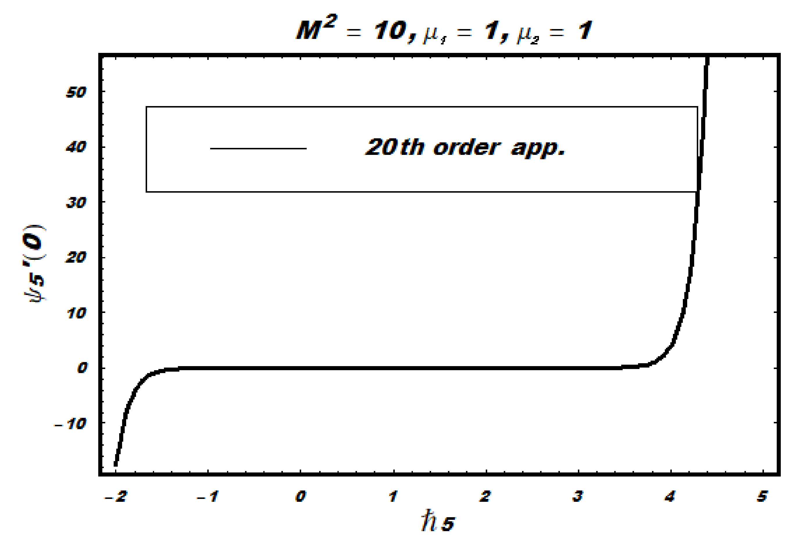
4. Convergence Criteria

HAM was applied to compute the solution of the problems given in Equations (7)–(9), (20), and (21), as HAM contains the non-zero auxiliary parameter i ( i = 1 5 ) , which ensures the convergence of the solution. To get a suitable value for the i , i curves are displayed. To guarantee the convergence, 20th order i curves have been drawn in Figure 2, Figure 3, Figure 4, Figure 5 and Figure 6. It can easily be seen from the i curves that the acceptable values of i were 0.5 1 1.5 ,     1.5 2 0.5 ,    0 3 6 , for the long slider. Similarly, acceptable values for the circular slider were 0.5 4 1.5 ,    1 5 4.

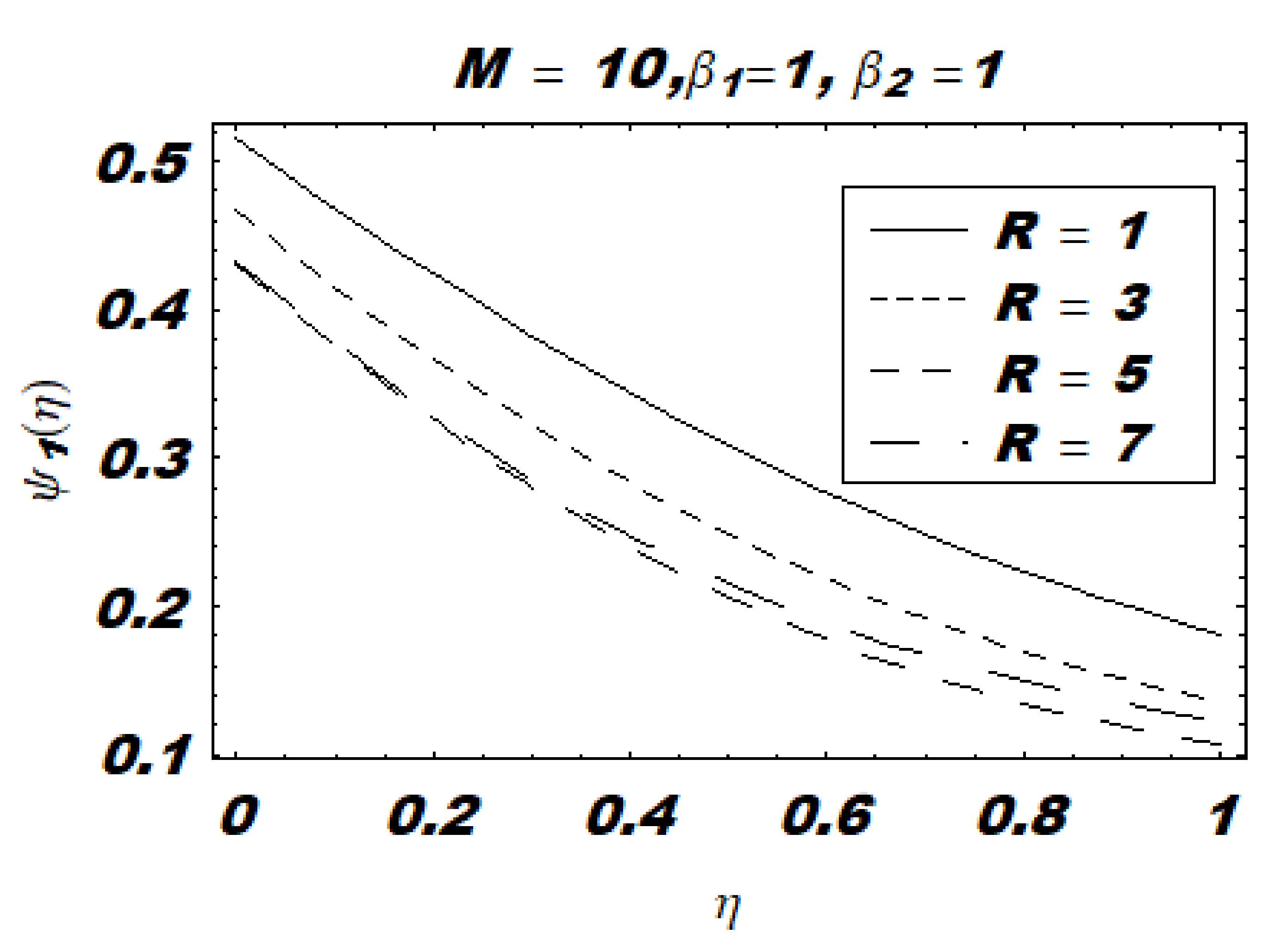
5. Results and Discussion

The obtained results from the above-mentioned method (HAM) are presented in the form of tables and graphs. Table 1 and Table 2 display the effects of the slip on the dynamic properties of a slider, showing that normalized lift and drag decrease as the slip and/or Reynolds number increases. The lift (per area) of the strip slider was much greater than the circular slider, although the drag remained the same in both cases. The effect of slip could be substantial, affecting the drag much more than the lift.
Velocity distributions for the long and circular slider are presented graphically in Figure 7, Figure 8 and Figure 9.
For the long slider, the effect of the Reynolds number in the presence of slip and the magnetic field is shown in Figure 10, Figure 11, Figure 12, Figure 13, Figure 14, Figure 15, Figure 16, Figure 17 and Figure 18. It is observed that the velocity profile was very much changed. It was seen that slip near the ground reduced the lateral velocity much more than slip on the slider. Moreover, increasing the magnetic parameter decreased the lateral velocity components further (see Figure 12). The effects of the Reynolds number on the typical velocity distribution for the circular slider were similar, as displayed in Figure 19, Figure 20, Figure 21, Figure 22, Figure 23, Figure 24, Figure 25, Figure 26, Figure 27 and Figure 28. The behavior of velocity profiles was similar for the long and circular sliders in cases of no-slip (see Figure 19 and Figure 20). Further, velocity profiles behaved in a similar fashion in both cases (i.e., parabolic or linear for a low Reynolds number, while a boundary layer formed near the surface in cases of a large Reynolds number). Figure 21, Figure 22, Figure 23, Figure 24, Figure 25, Figure 26, Figure 27 and Figure 28 demonstrate the effect of the slip parameter on the velocity components corresponding to different Reynolds numbers. These pictorial descriptions demonstrate that velocity profiles decrease with an increase in slip parameters, and that this decrease become even greater after applying the magnetic field. This is due to the fact that slip hinders fluid particles and displaces motion in the vicinity.
These results qualitatively confirm the expectation that a drag-like Lorentz force is created by the magnetic field normal to the lateral flow direction, and this force decreases the lateral velocity components. Lift and drag components are important physical quantities for a porous slider. It is interesting to note that the lift is free of translation, but the drag components depend on a cross flow. The effectiveness of a porous slider can be enhanced by making the ratio of friction force to lift smaller. As pointed out by Wang [16], the porous slider should be operated at a cross-flow Reynolds number below unity for optimum efficiency. According to Table 1, porous sliders should be operated at small values that are still valid even when an external uniform magnetic field is applied. Moreover, from the point of view of optimum efficiency, it is more efficient to move a flat slider on a fluid subject than in a high-intensity magnetic field.

6. Conclusions

In this research, different studies have been complied altogether. Different researchers have analyzed fluid flow on a long slider without slip, while others were interested only in a circular slider without slip. Wang presented a comparative study of the both sliders and added velocity slip, but did not cover the effects of a magnetic field. As such, one concern of this study was theoretical investigation of a steady three-dimensional flow of a viscous fluid between a porous slider and the ground in the presence of a transverse uniform magnetic field with velocity slip. The effects of different physical parameter values like Reynolds number and magnetic field on the lateral velocity profiles and lift and drag components were presented in graphs and tables in the presence of velocity slip. It is expected that the results of the present study could be useful for the understanding of various technical problems related to porous sliders where magnetic and velocity slip are the main physical parameters. The main findings are as follows:
  • It was shown that normalized lift and drag go down as slip and/or the Reynolds number goes up (see Table 1 and Table 2). The lift (per area) of a long slider is much greater than a circular slider. The drag remains the same for both sliders.
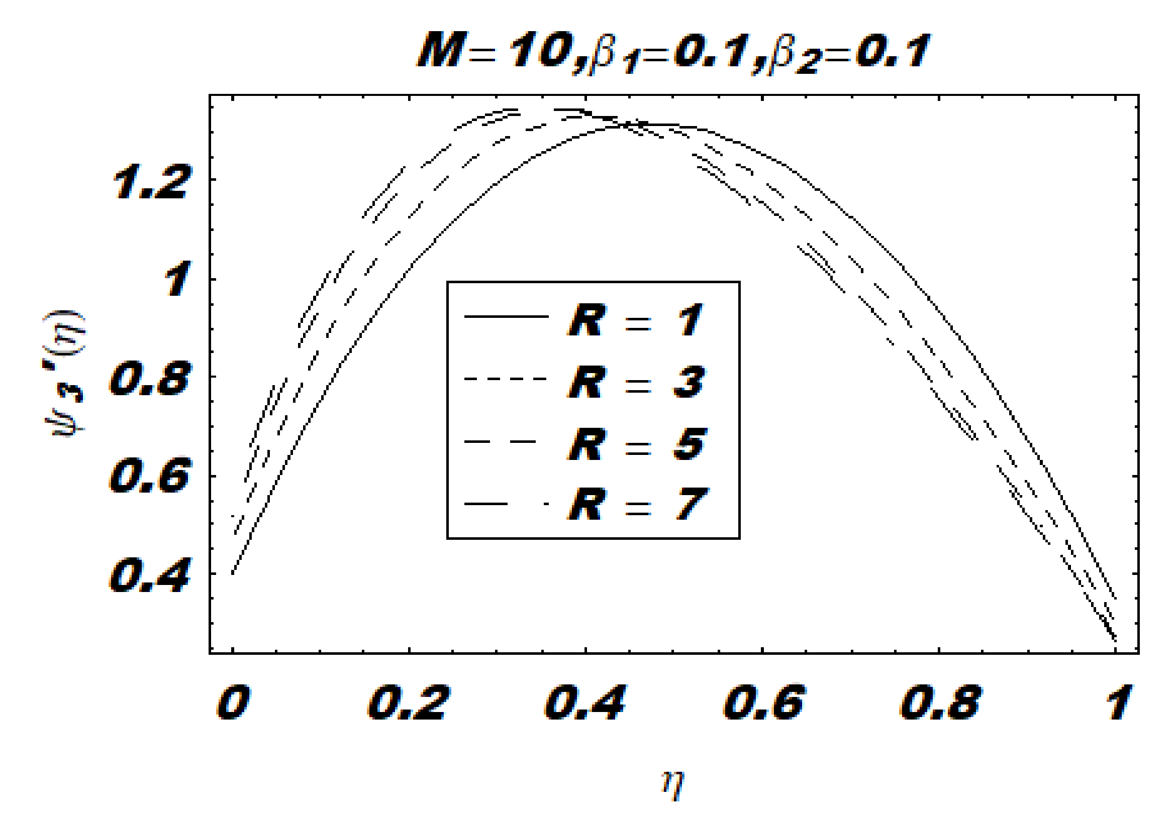
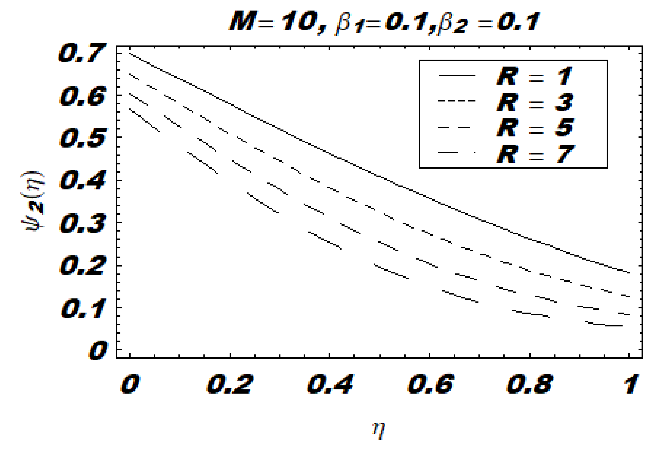
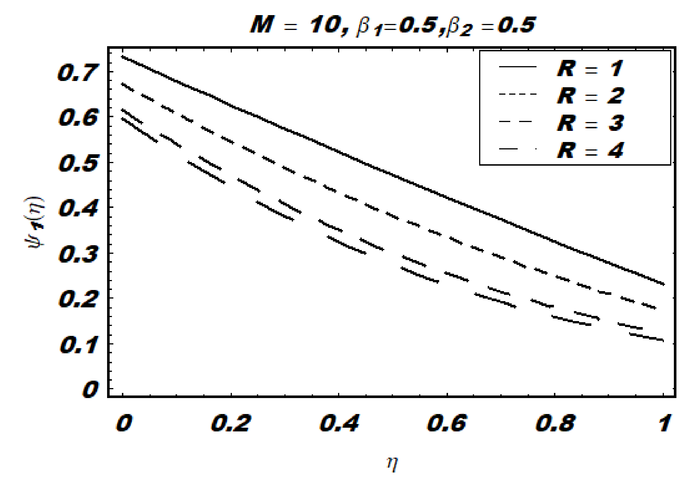
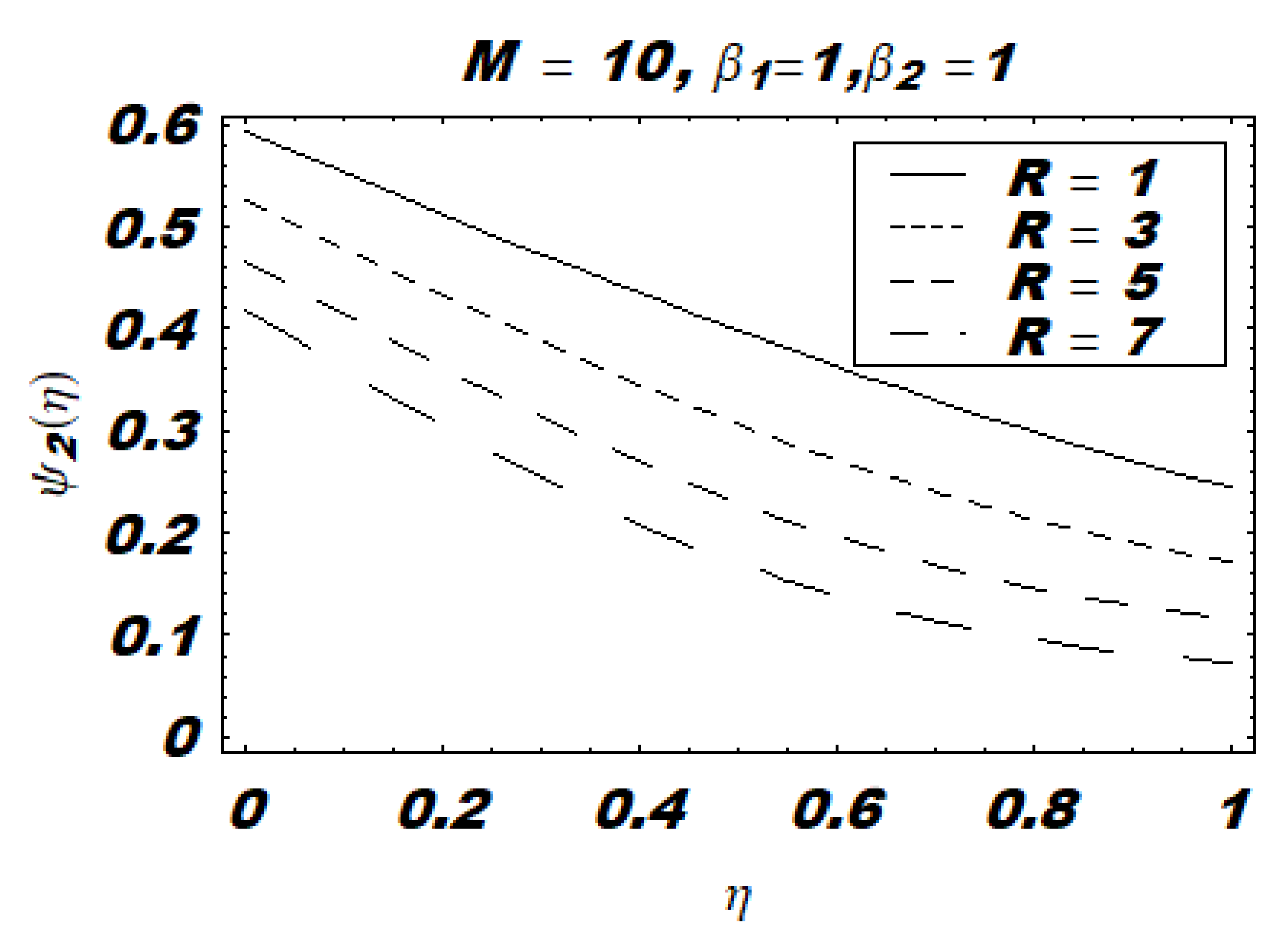
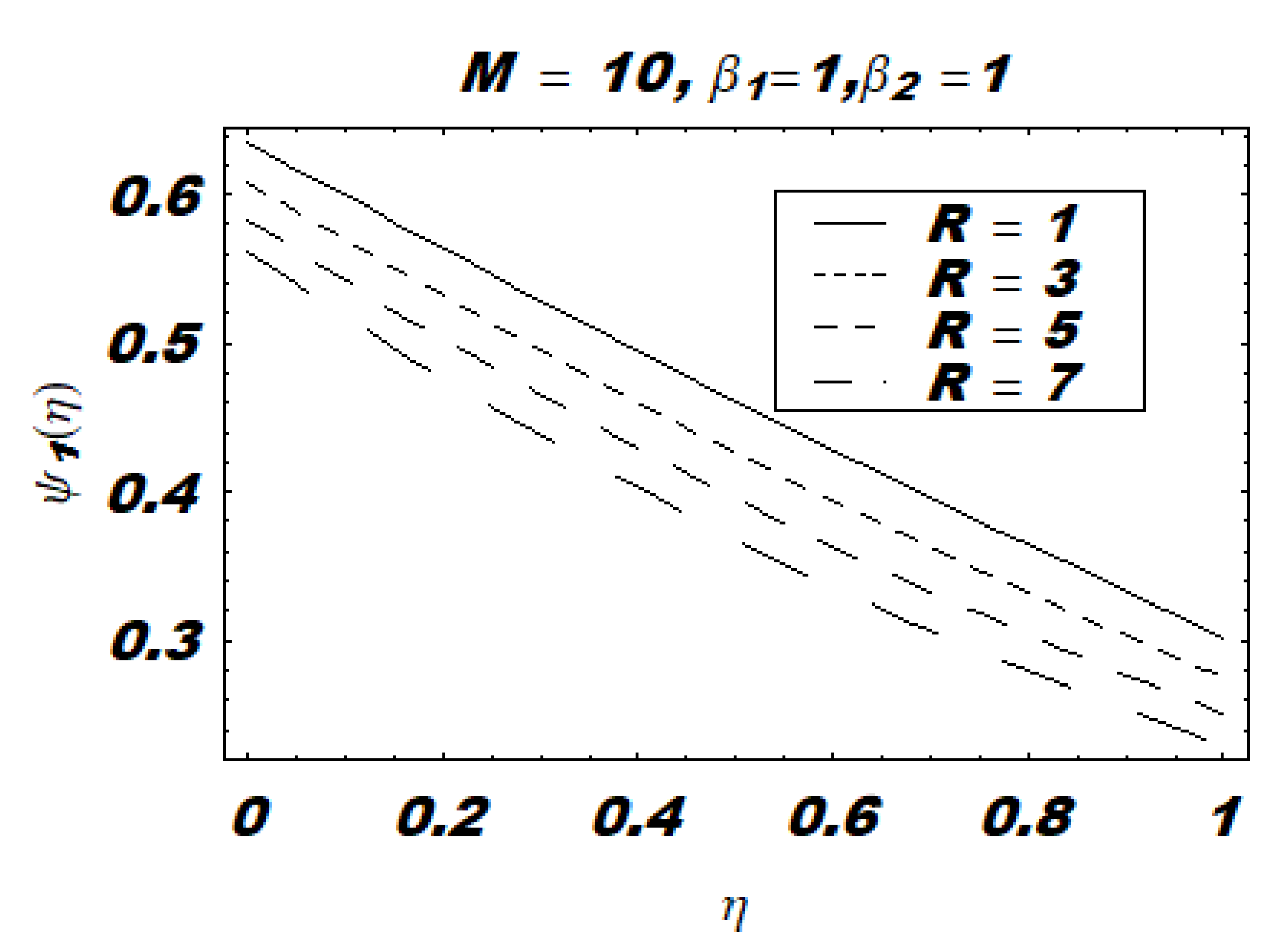
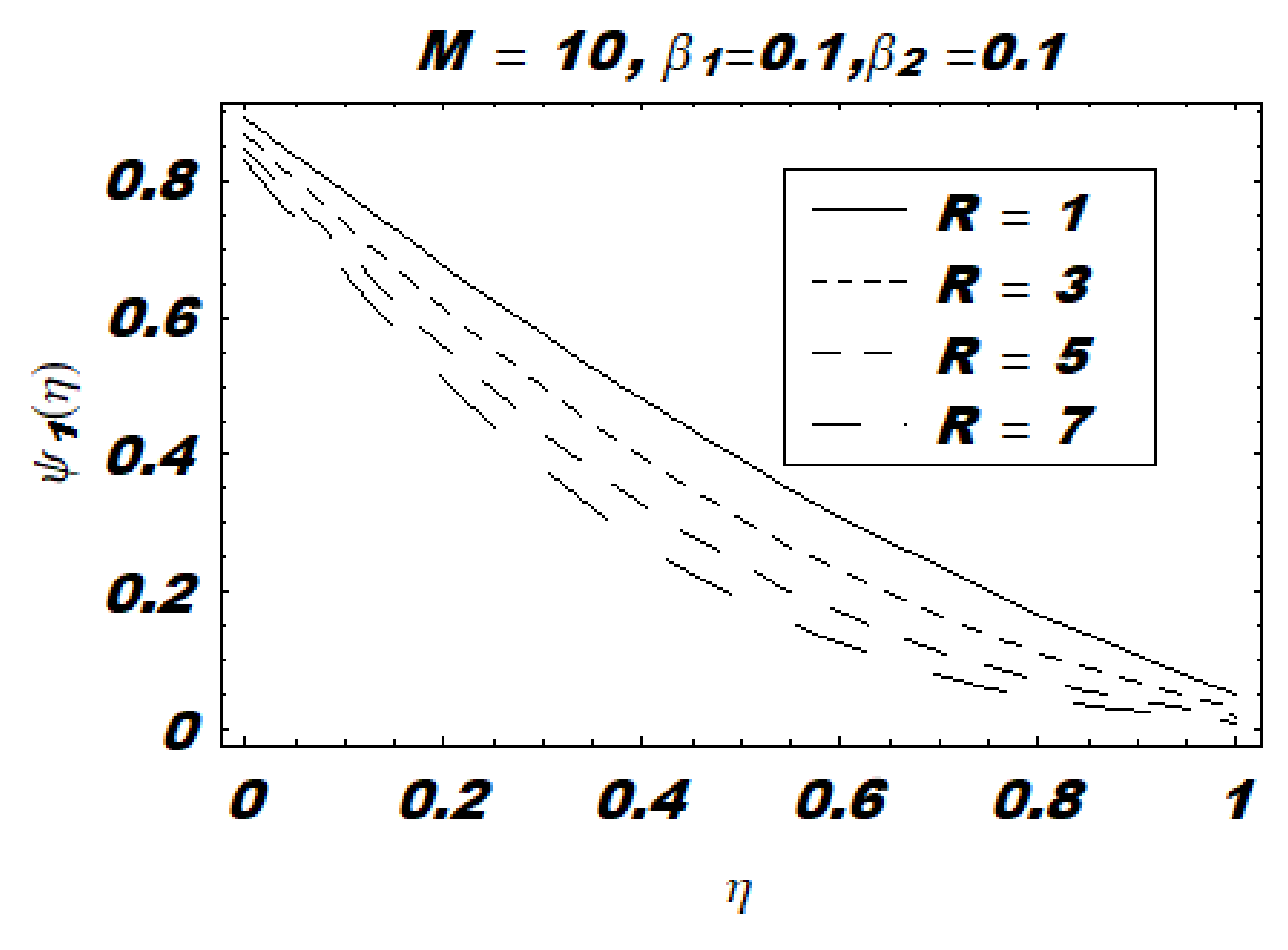
  • Slip near the ground reduces lateral velocity of the slider much more than slip. By increasing the magnetic parameter, the lateral velocity components decrease further.
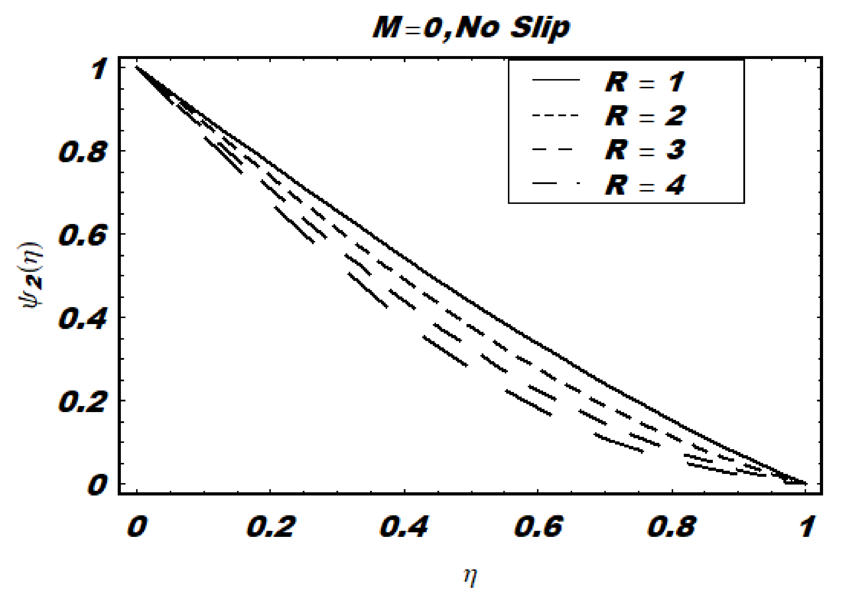
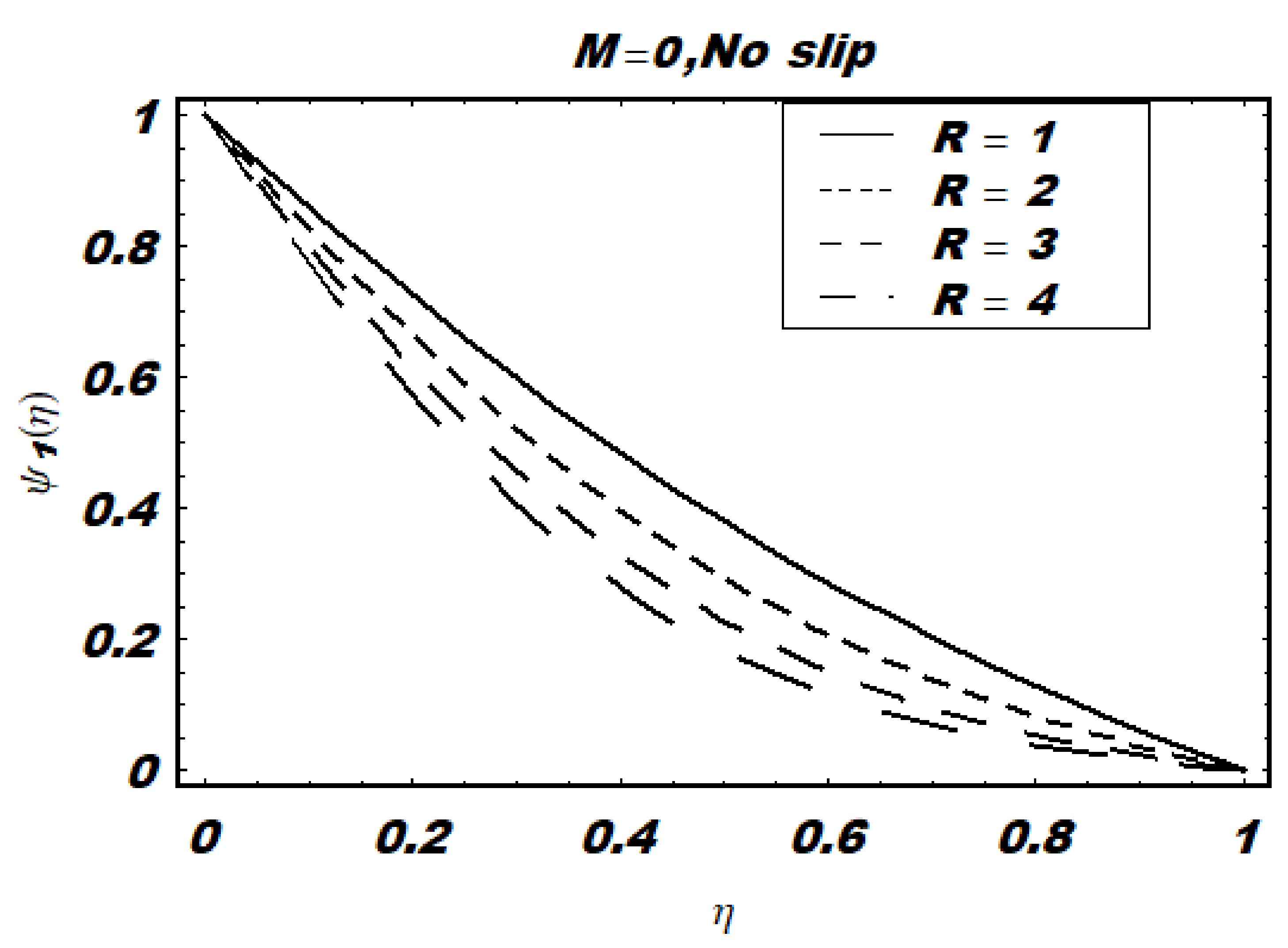
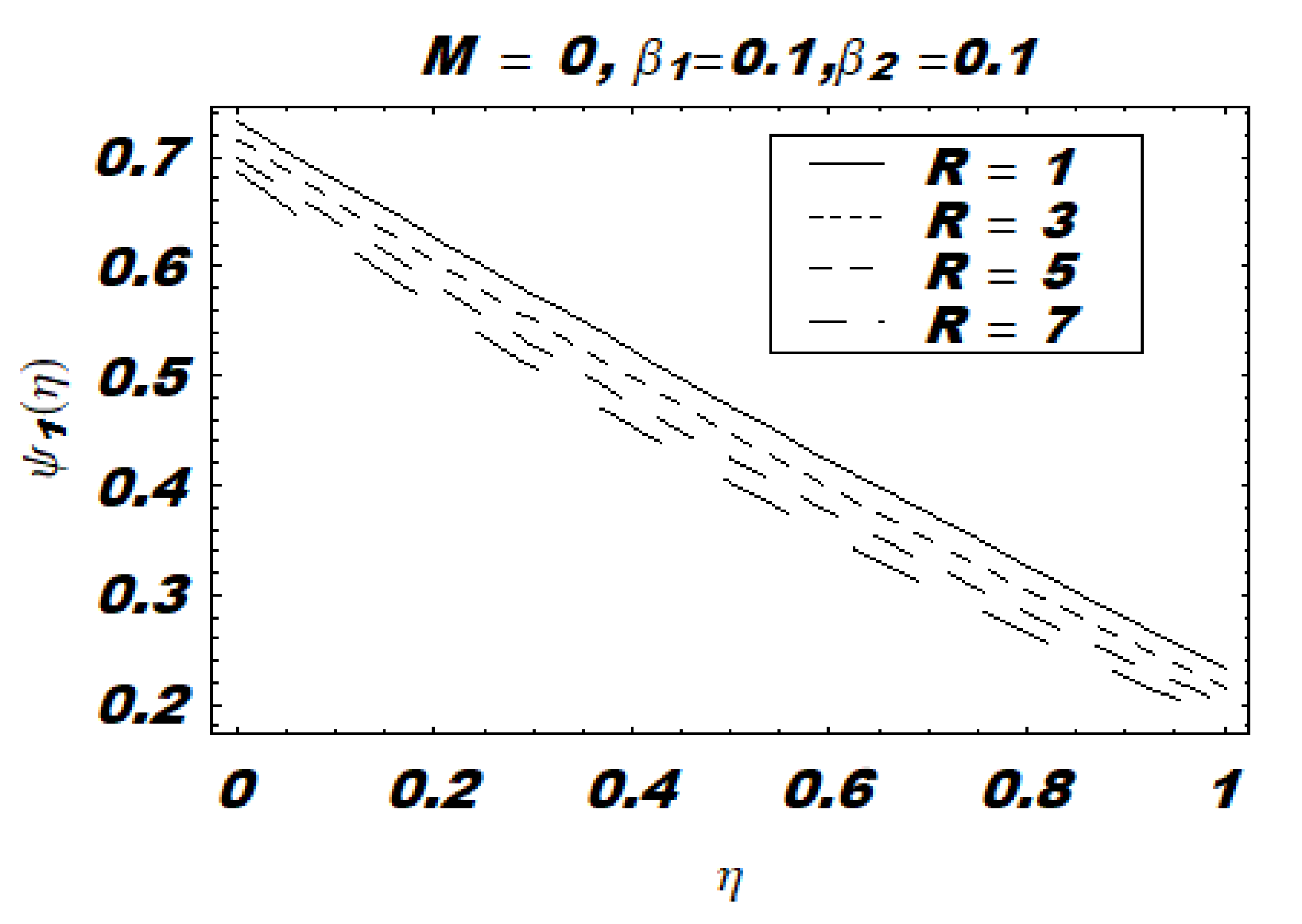
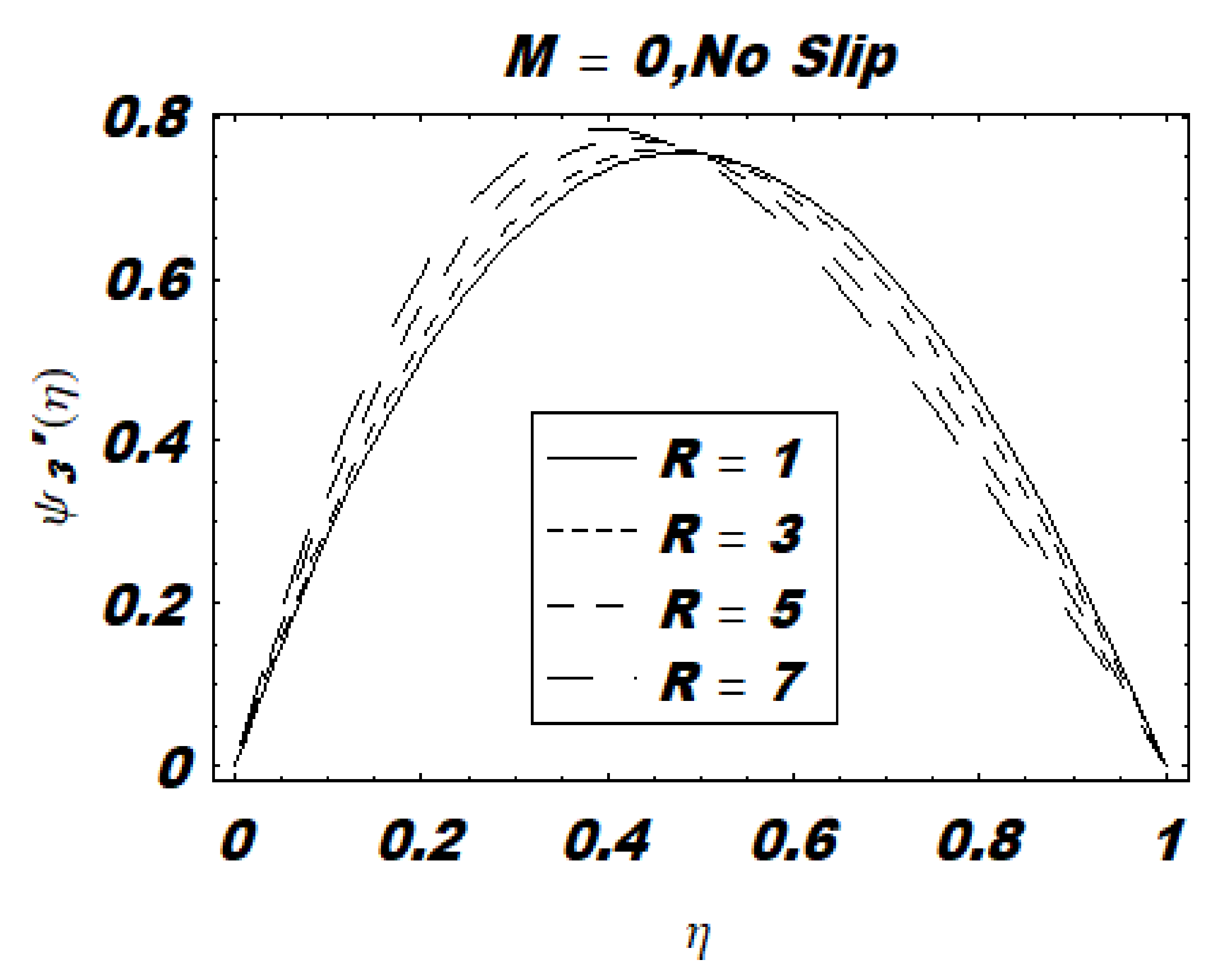
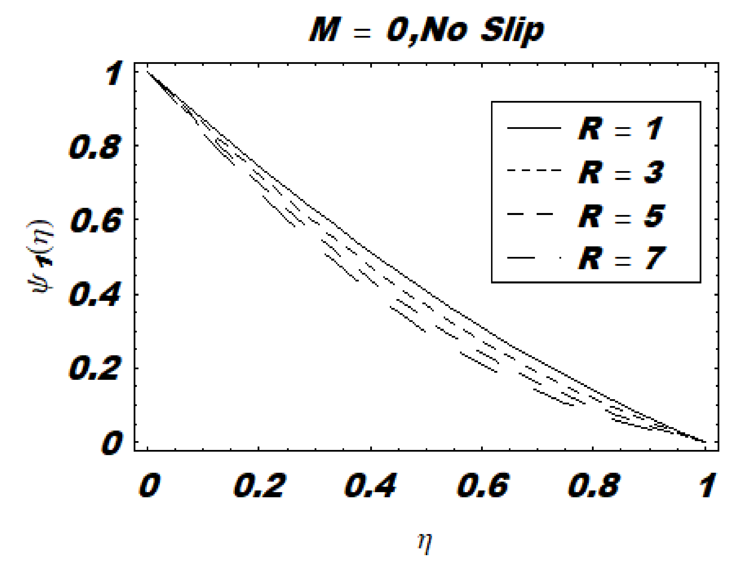
  • The behavior of velocity profiles is similar for the long and the circular sliders in cases of no-slip (i.e., parabolic or linear for a low Reynolds number).
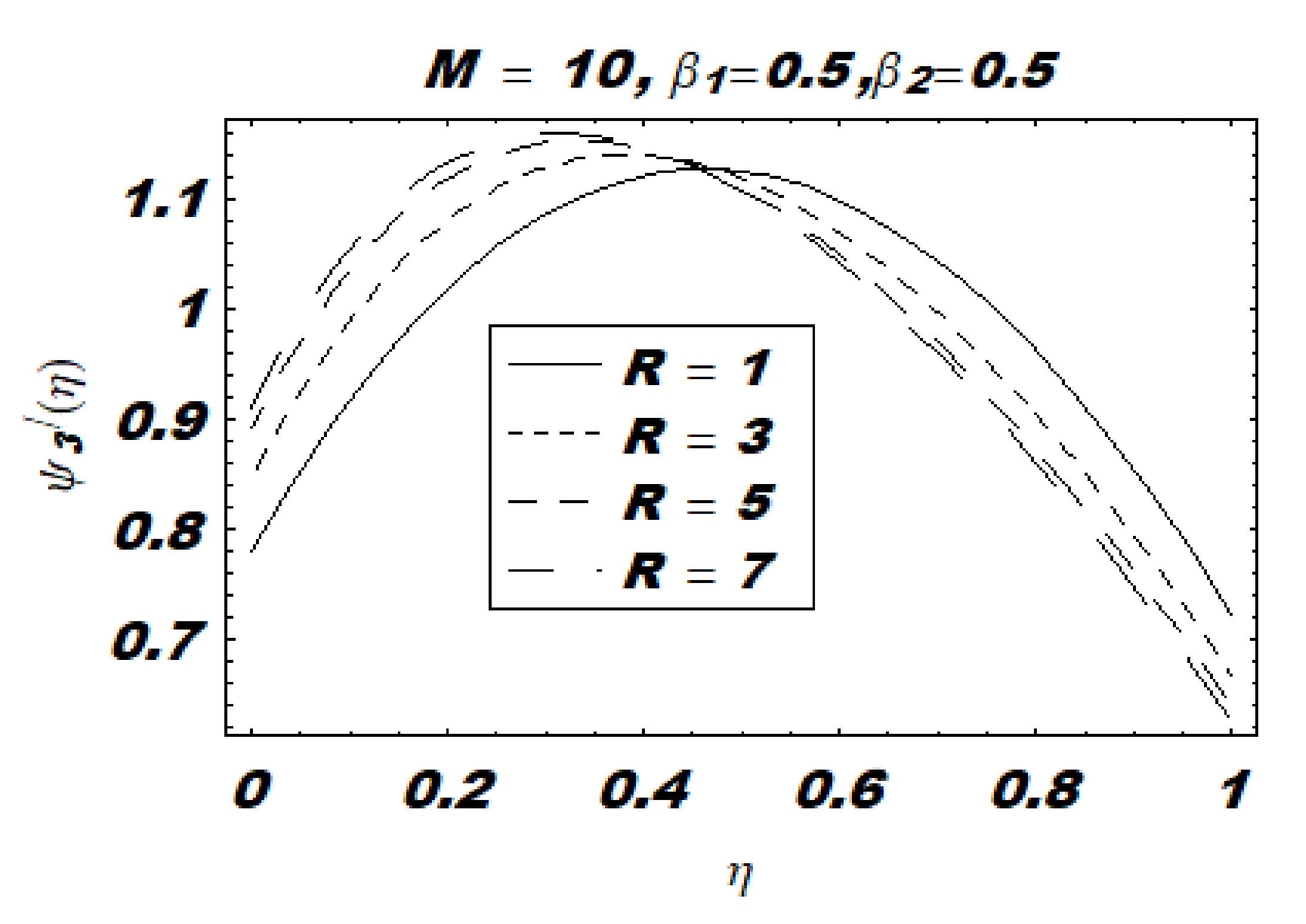
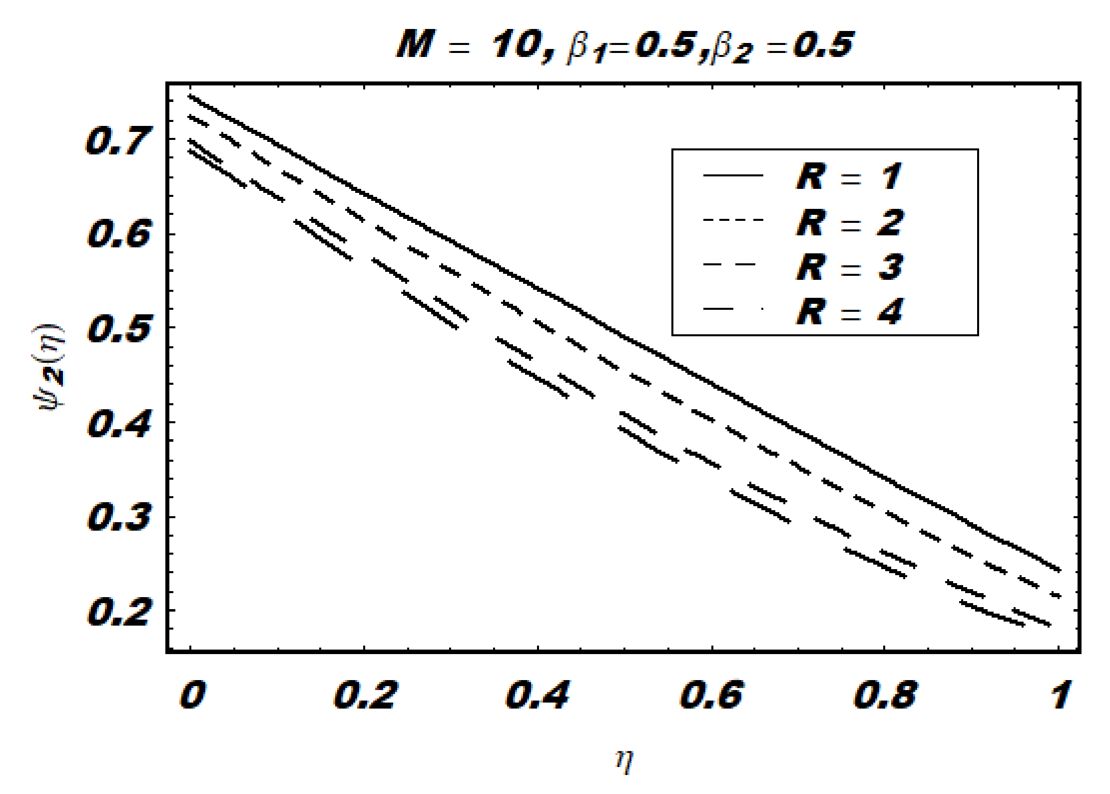
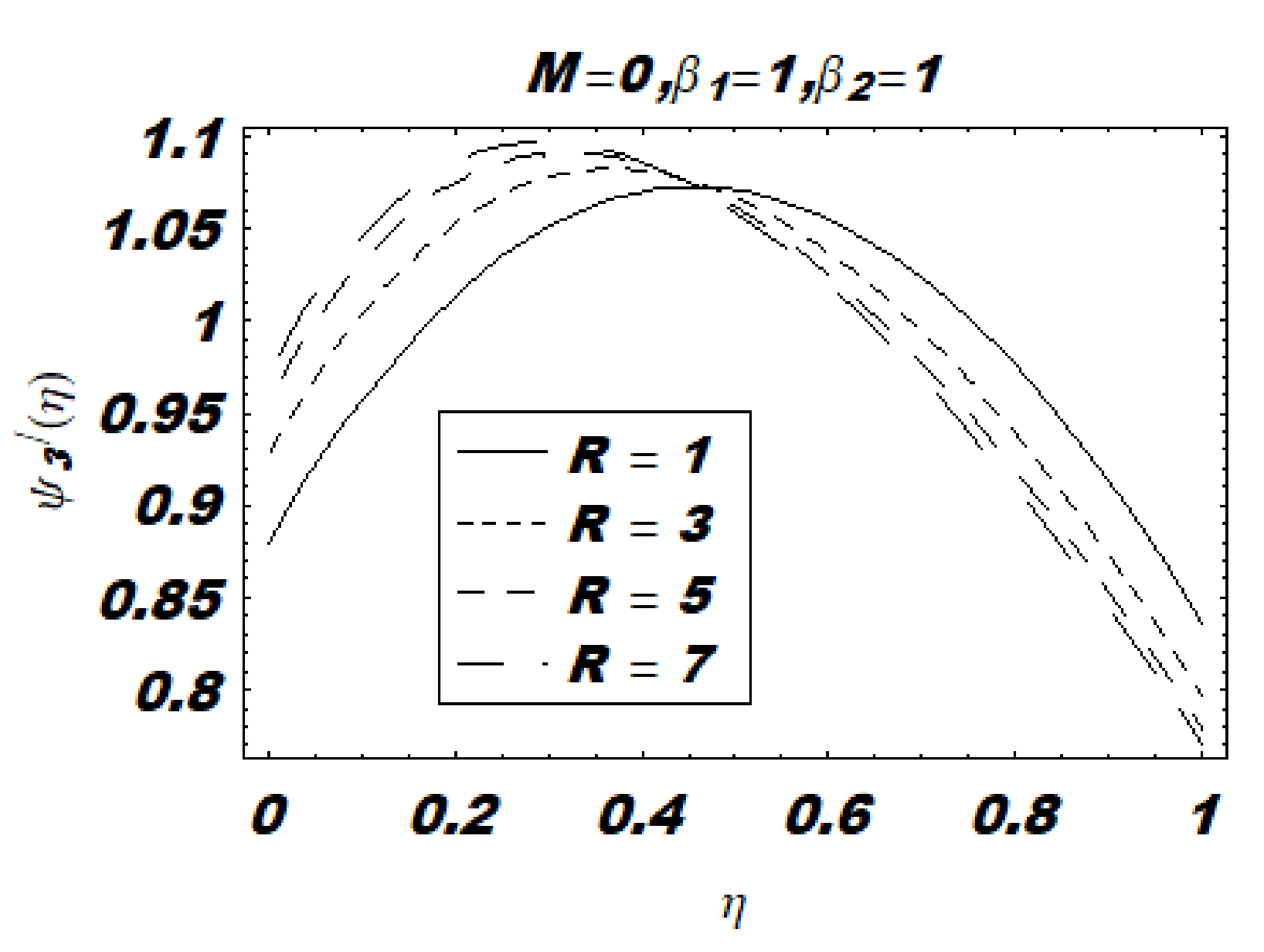
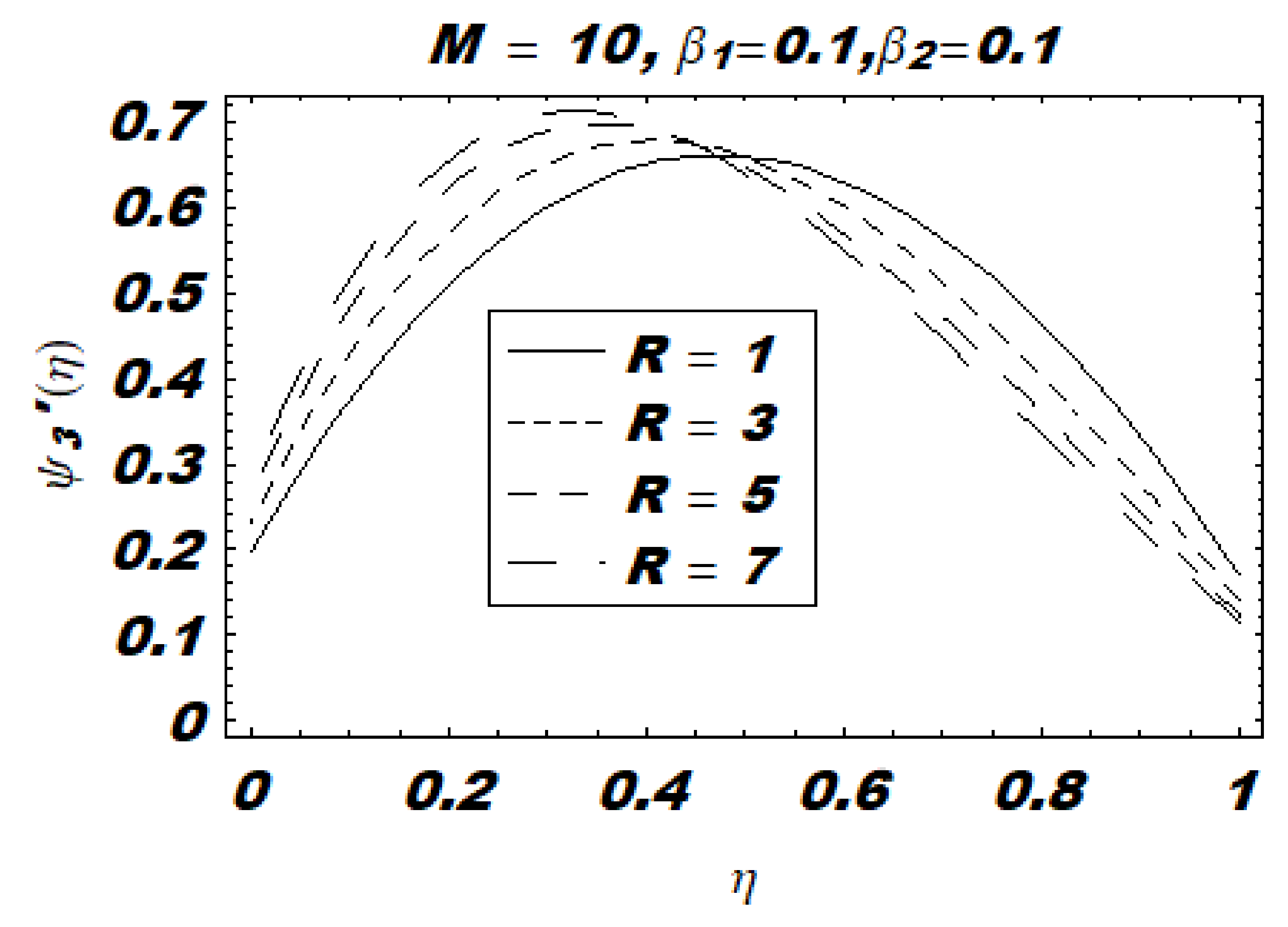
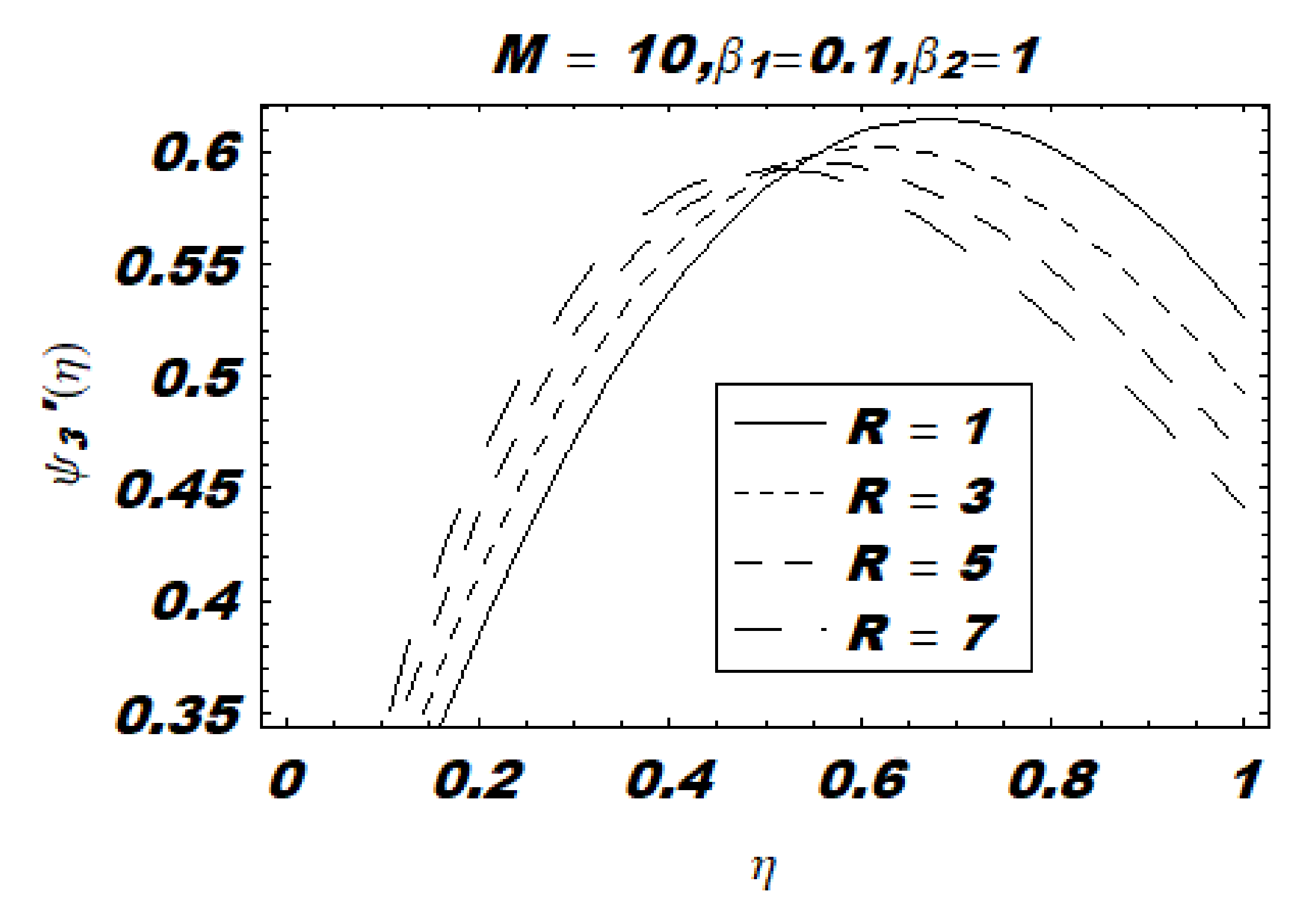
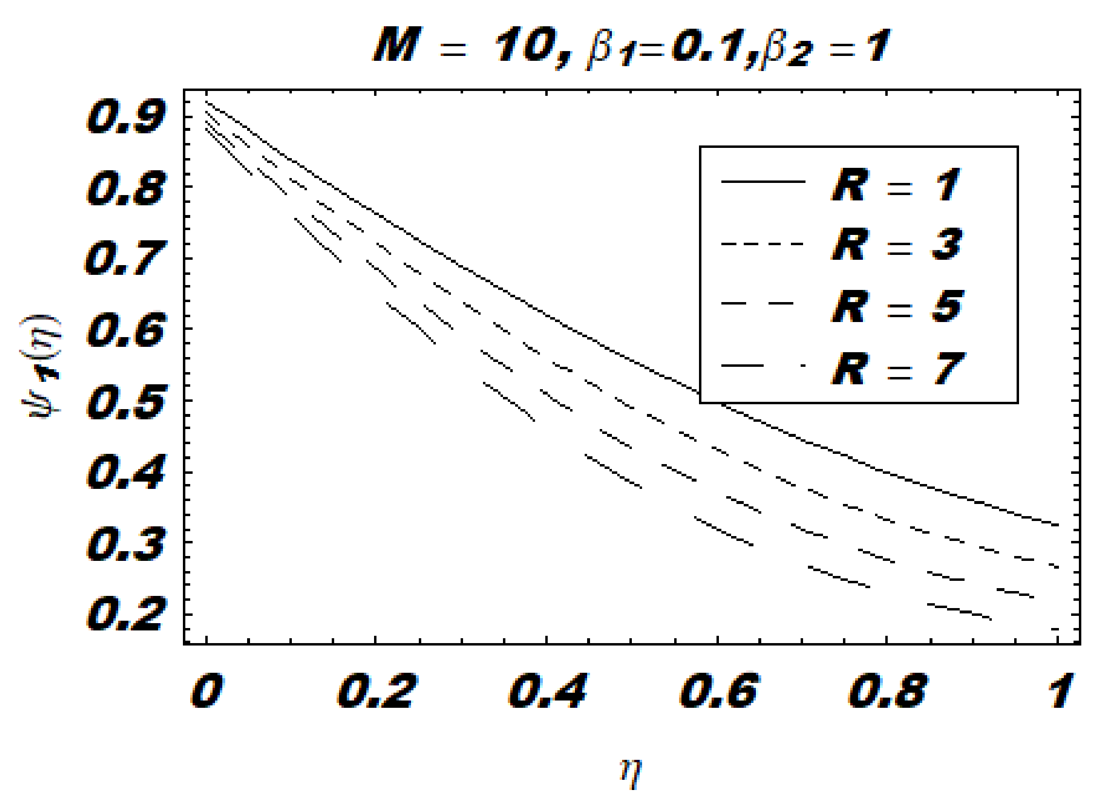
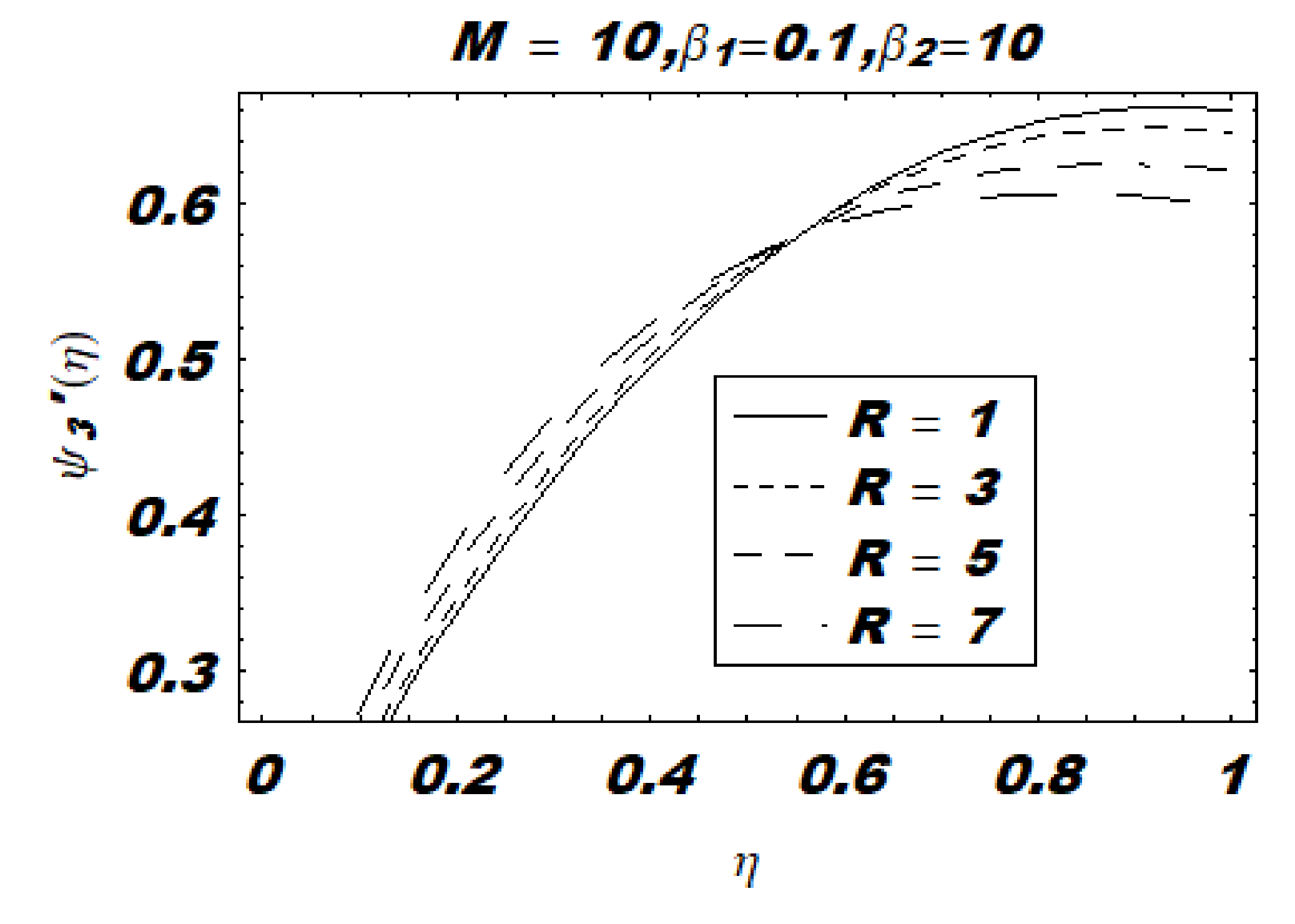
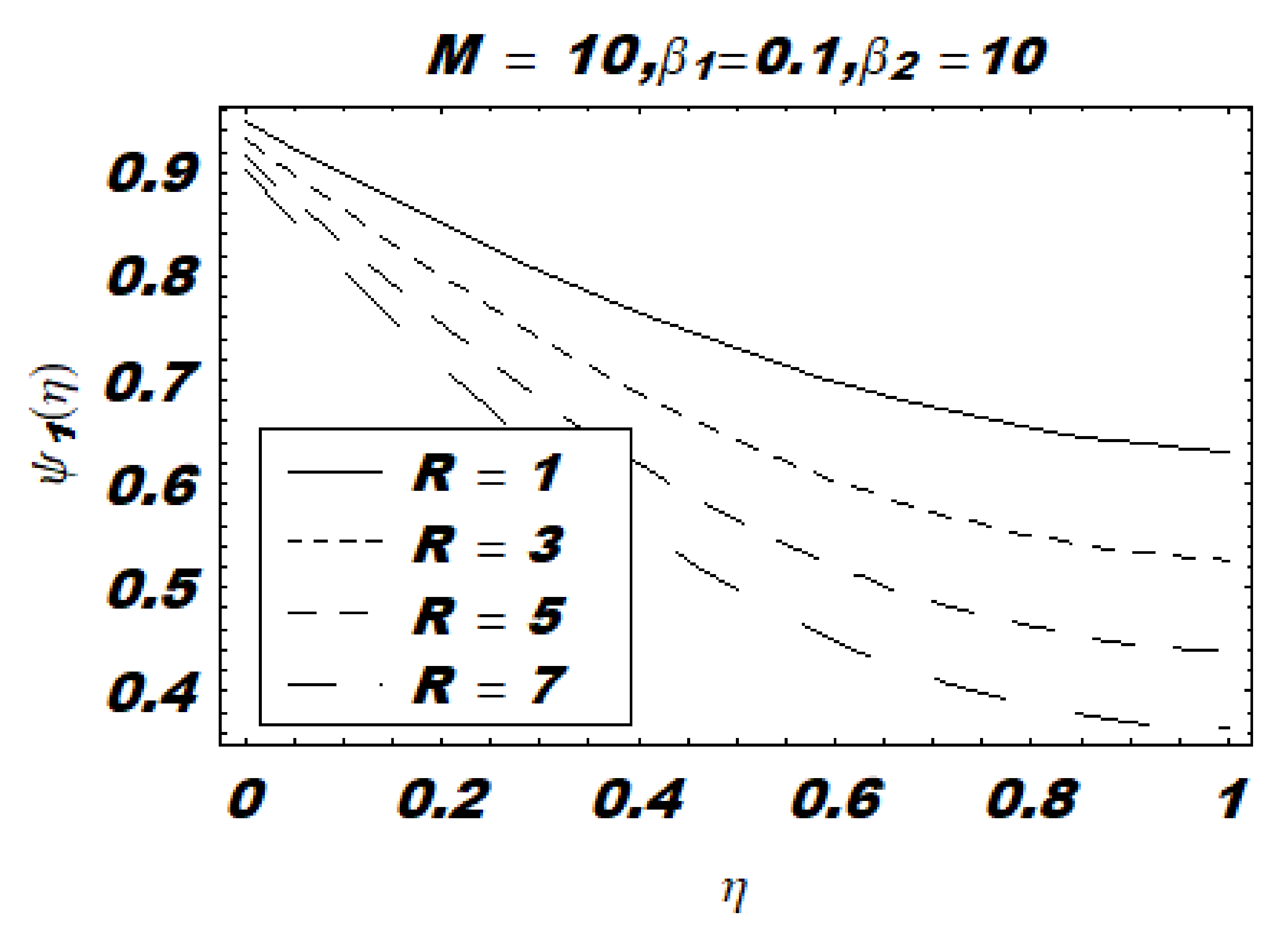
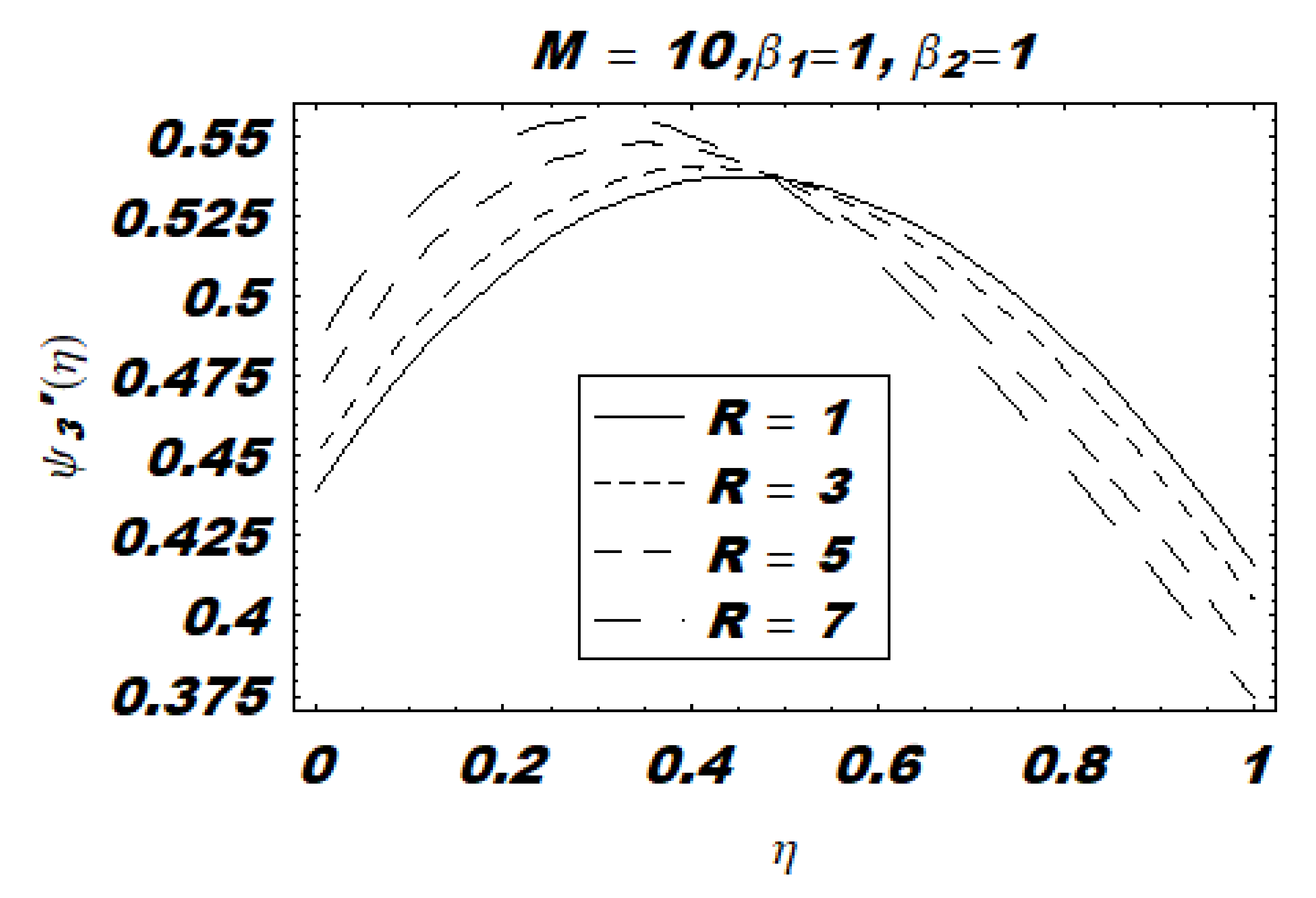
  • In cases of a large Reynolds number, a boundary layer formed near the surface, while velocity profiles decreased with an increase in slip parameters, a decrease which grew more pronounced after applying the magnetic field.

Author Contributions

N.F. and Y.K. conducted whole research such as preparation, creation and/or presentation of the published work by those from the original research group, specifically critical review, commentary or revision – including pre- or post-publication stages. A.A. helped to improve the language of the paper. Drew the schematic diagram of the problem, preparation, creation and/or presentation of the published work, specifically visualization/data presentation. M.K. helped to revise the reviewers’ comments.

Funding

This work was supported by the International Cultural Exchange School (ICES), Donghua University, West Yan’an Road 1882, Shanghai 200051, China.

Conflicts of Interest

The authors declare no conflict of interest.

Nomenclature

B 0 Magnetic field μ Dynamic viscosity
d Width η Similarity variable
H 1 , H 2 Slip coefficient τ Extra stress tensor
I Identity tensor β 1 , β 2 Slip factors
l Length ψ 1 , ψ 2 , ψ 3 Velocity function
p Pressure ϕ 1 , ϕ 2 , ϕ 3 Velocity components
v 0 Constant viscosity ρ Fluid density
x 1 , x 2 , x 3 Space coordinates

References

  1. Skalak, F.; Wang, C.-Y. Fluid Dynamics of a Long Porous Slider. J. Appl. Mech. 1975, 42, 893–894. [Google Scholar] [CrossRef]
  2. Wang, C.-Y. Erratum: “Fluid Dynamics of the Circular Porous Slider.” J. Appl. Mech. 1974, 41, 343–347. J. Appl. Mech. 1978, 45, 236. [Google Scholar] [CrossRef]
  3. Wang, C.-Y. The Elliptic Porous Slider at Low Crossflow Reynolds Numbers. J. Lubr. Technol. 1978, 100, 444. [Google Scholar] [CrossRef]
  4. Bhattacharjee, R.C.; Das, N.C. Porous slider bearing lubricated with couple stress mhd fluids. Trans. Can. Soc. Mech. Eng. 1994, 18, 317–331. [Google Scholar] [CrossRef]
  5. Patel, J.R.; Deheri, G. A study of thin film lubrication at nanoscale for a ferrofluid based infinitely long rough porous slider bearing. Facta Univ. Ser. Mech. Eng. 2016, 14, 89–99. [Google Scholar] [CrossRef]
  6. Sinha, P.; Adamu, G. Analysis of Thermal Effects in a Long Porous Rough Slider Bearing. Proc. Natl. Acad. Sci. India Sectoin A Phys. Sci. 2017, 87, 279–290. [Google Scholar] [CrossRef]
  7. Munshi, M.M.; Patel, A.R.; Deheri, G. Analysis of Rough Porous Inclined Slider Bearing Lubricated with a Ferrofluid Considering Slip Velocity. Int. J. Res. Advent Technol. 2019, 7, 387–396. [Google Scholar]
  8. Lang, J.; Nathan, R.; Wu, Q. Theoretical and experimental study of transient squeezing flow in a highly porous film. Tribol. Int. 2019, 135, 259–268. [Google Scholar] [CrossRef]
  9. Madalli, V.S.; Bujurke, N.M.; Mulimani, B.G. Lubrication of a long porous slider. Tribol. Int. 1995, 28, 225–232. [Google Scholar] [CrossRef]
  10. Awati, V.B.; Jyoti, M. Homotopy analysis method for the solution of lubrication of a long porous slider. Appl. Math. Nonlinear Sci. 2016, 1, 507–516. [Google Scholar] [CrossRef] [Green Version]
  11. Khan, Y.; Faraz, N.; Yildirim, A.; Wu, Q. A Series Solution of the Long Porous Slider. Tribol. Trans. 2011, 54, 187–191. [Google Scholar] [CrossRef]
  12. Khan, Y.; Wu, Q.; Faraz, N.; Mohyud-Dind, S.T.; Yıldırım, A. Three-Dimensional Flow Arising in the Long Porous Slider: An Analytic Solution. Z. Nat. A 2011, 66, 507–511. [Google Scholar]
  13. Faraz, N.; Khan, Y.; Lu, D.C.; Goodarzi, M. Integral transform method to solve the problem of porous slider without velocity slip. Symmetry 2019, 11, 791. [Google Scholar] [CrossRef]
  14. Ghoreishi, M.; Ismail, A.I.B.M.; Rashid, A. The One Step Optimal Homotopy Analysis Method to Circular Porous Slider. Math. Probl. Eng. 2012, 2012, 135472. [Google Scholar] [CrossRef]
  15. Shukla, S.D.; Deheri, G.M. Rough porous circular convex pad slider bearing lubricated with a magnetic fluid. In Lecture Notes in Mechanical Engineering; Springer: Berlin/Heidelberg, Germany, 2014. [Google Scholar]
  16. Wang, C.Y. A porous slider with velocity slip. Fluid Dyn. Res. 2012, 44, 065505. [Google Scholar] [CrossRef]
  17. Wang, C.-Y. Fluid Dynamics of the Circular Porous Slider. J. Appl. Mech. 1974, 41, 343. [Google Scholar] [CrossRef]
  18. Faraz, N. Study of the effects of the Reynolds number on circular porous slider via variational iteration algorithm-II. Comput. Math. Appl. 2011, 61, 1991–1994. [Google Scholar] [CrossRef] [Green Version]
  19. Madani, M.; Khan, Y.; Mahmodi, G.; Faraz, N.; Yildirim, A.; Nasernejad, B. Application of homotopy perturbation and numerical methods to the circular porous slider. Int. J. Numer. Methods Heat Fluid Flow 2012, 22, 705–717. [Google Scholar] [CrossRef]
  20. Naeem, F.; Yasir, K. Thin film flow of an unsteady Maxwell fluid over a shrinking/stretching sheet with variable fluid properties. Int. J. Numer. Methods Heat Fluid Flow 2018, 28, 1596–1612. [Google Scholar]
Figure 1. (a) Schematic diagram of the movement of a long porous slider (LPS). (b) Schematic diagram of the movement of a circular porous slider (CPS).
Mathematics 07 00748 g001
Figure 2. 1 for the strip/long slider.
Mathematics 07 00748 g002
Figure 3. 2 for the strip/long slider.
Mathematics 07 00748 g003
Figure 4. 3 for the strip/long slider.
Mathematics 07 00748 g004
Figure 5. 4 for the circular slider.
Mathematics 07 00748 g005
Figure 6. 5 for the circular slider.
Mathematics 07 00748 g006
Figure 7. Similarity function ψ 3 / for the long slider.
Mathematics 07 00748 g007
Figure 8. Similarity function ψ 2 for the long slider.
Mathematics 07 00748 g008
Figure 9. Similarity function ψ 1 for the long slider.
Mathematics 07 00748 g009
Figure 10. Similarity function ψ 3 / for the long slider.
Mathematics 07 00748 g010
Figure 11. Similarity function ψ 2 for the long slider.
Mathematics 07 00748 g011
Figure 12. Similarity function ψ 1 for the long slider.
Mathematics 07 00748 g012
Figure 13. Similarity function ψ 3 / for the long slider.
Mathematics 07 00748 g013
Figure 14. Similarity function ψ 2 for the long slider.
Mathematics 07 00748 g014
Figure 15. Similarity function ψ 1 for the long slider.
Mathematics 07 00748 g015
Figure 16. Similarity function ψ 3 / for the long slider.
Mathematics 07 00748 g016
Figure 17. Similarity function ψ 1 for the long slider.
Mathematics 07 00748 g017
Figure 18. Similarity function ψ 3 / for the long slider.
Mathematics 07 00748 g018
Figure 19. Similarity function ψ 3 / for the circular slider.
Mathematics 07 00748 g019
Figure 20. Similarity function ψ 1 for the circular slider.
Mathematics 07 00748 g020
Figure 21. Similarity function ψ 3 / for the circular slider.
Mathematics 07 00748 g021
Figure 22. Similarity function ψ 1 for the circular slider.
Mathematics 07 00748 g022
Figure 23. Similarity function ψ 3 / for the circular slider.
Mathematics 07 00748 g023
Figure 24. Similarity function ψ 1 for the circular slider.
Mathematics 07 00748 g024
Figure 25. Similarity function ψ 3 / for the circular slider.
Mathematics 07 00748 g025
Figure 26. Similarity function ψ 1 for the circular slider.
Mathematics 07 00748 g026
Figure 27. Similarity function ψ 3 / for the circular slider.
Mathematics 07 00748 g027
Figure 28. Similarity function ψ 1 for the circular slider.
Mathematics 07 00748 g028
Table 1. Properties of the long porous slider. Normalized lift Λ , normalized x 1 direction drag, and normalized x 2 direction drag.
β 1 , β 2 M 2 R Λ ψ 1 / ( 1 ) ψ 2 / ( 1 )
0, 000.262.330.8960.932
--0.526.340.7600.836
--2.08.4120.3340.467
--5.04.9170.0630.123
--203.26700
--502.90900
0.1, 0.120.239.270.7430.780
-40.516.780.6260.704
-62.06.5960.43720.2536
-105.03.4360.32450
2020.02.4400.15200
5050.02.24000
0.1, 120.220.310.4240.463
-40.58.8590.3570.436
-62.03.1590.1600.321
-105.02.0500.0350.123
2020.01.51300.0632
5050.01.39100.012
0.1, 1020.25.3160.0640.082
-40.52.7020.0460.080
-62.01.4130.0130
-105.01.1750.0020
2020.01.06800
5050.01.04700
1, 120.29.7270.2750.315
-40.54.5910.2100.288
-62.02.0480.0680.172
105.01.5690.0110.047
2020.01.35500
5050.01.31500
Table 2. Properties of the circular porous slider. Normalized lift Λ , normalized drag ψ 1 / ( 1 ) .
β 1 , β 2 M 2 R Λ ψ 1 / ( 1 )
0, 000.230.780.914
--0.512.790.797
--2.03.8330.392
--5.02.0190.085
--201.3490
--501.1940
0.1, 0.120.219.330.761
-40.58.0890.663
-62.02.5030.310
-105.01.4450.1014
2020.00.9940
5050.00.9080
0.1, 120.29.8530.441
-40.54.1300.394
-62.01.2880.129
-105.00.7520.0145
2020.00.5290
5050.00.4830
0.1, 1020.26.4380.084
-40.52.6990.076
-62.00.8410.015
-105.00.4880
2020.00.3380
5050.00.3050
1, 120.24.6110.294
-40.52.0430.244
-62.00.7760.0215
105.00.5490
2020.00.4660
5050.00.4530

