Article

New Polynomial Bounds for Jordan’s and Kober’s Inequalities Based on the Interpolation and Approximation Method

1
School of Computer Science and Technology, Henan Polytechnic University, Jiaozuo 454000, China
2
School of Mathematics and Information Science, Henan Polytechnic University, Jiaozuo 454000, China
*
Author to whom correspondence should be addressed.
Mathematics 2019, 7(8), 746; https://doi.org/10.3390/math7080746
Submission received: 4 July 2019 / Revised: 10 August 2019 / Accepted: 13 August 2019 / Published: 15 August 2019

Abstract

:
In this paper, new refinements and improvements of Jordan’s and Kober’s inequalities are presented. We give new polynomial bounds for the s i n c ( x ) and cos ( x ) functions based on the interpolation and approximation method. The results show that our bounds are tighter than the previous methods.

1. Introduction

Jordan’s inequality:
2 π s i n c ( x ) = sin ( x ) x < 1 , x ( 0 , π / 2 ] ,
has been studied in a large number of literature works, and many refinements have been presented [1,2,3,4,5,6].
Zhang et al. [7] gave the polynomial bounds of degree one:
2 π + π 2 π 2 ( π 2 x ) sin ( x ) x 2 π + 2 π 2 ( π 2 x ) , x ( 0 , π / 2 ] .
Zhang and Ma [8] gave the improvement of Inequality (2):
1 + 4 2 π π 2 x sin ( x ) x 8 2 2 π 2 π + 2 2 8 2 π 2 x , x ( 0 , π / 2 ] .
Qi et al. [9] presented the polynomial bounds of degree two:
2 π + 1 π 3 ( π 2 4 x 2 ) sin ( x ) x 2 π + π 2 π 3 ( π 2 4 x 2 ) , x ( 0 , π / 2 ] .
Zhang and Ma [8] gave the improvement of Inequality (4):
1 + 12 4 π π 2 x + 4 π 16 π 3 x 2 sin ( x ) x 1 + 8 4 π π 3 x 2 , x ( 0 , π / 2 ] .
Deng [10] obtained the polynomial bounds of degree three:
2 π + 2 3 π 4 ( π 3 8 x 3 ) sin ( x ) x 2 π + π 2 π 4 ( π 3 8 x 3 ) , x ( 0 , π / 2 ] ,
and Jiang and Yun [11] gave the polynomial bounds of degree four:
2 π + 1 2 π 5 ( π 4 16 x 4 ) sin ( x ) x 2 π + π 2 π 5 ( π 4 16 x 4 ) , x ( 0 , π / 2 ] .
Debnath et al. [12] gave the improvements of Inequality (4) and Inequality (7):
g 4 , D 1 l ( x ) sin ( x ) x g 4 , D 1 u ( x ) , x ( 0 , π / 2 ] ,
and:
g 4 , D 2 l ( x ) sin ( x ) x g 4 , D 2 u ( x ) , x ( 0 , π / 2 ] ,
where
  • g 4 , D 1 l ( x ) = 2 π + 1 π 3 ( π 2 4 x 2 ) + ( 1 3 π ) ( 1 6 4 π 3 ) x 2 ,
  • g 4 , D 1 u ( x ) = 2 π + 1 π 3 ( π 2 4 x 2 ) + ( 1 3 π ) ( 1 6 4 π 3 ) x 2 + 1 120 x 4 ,
  • g 4 , D 2 l ( x ) = 2 π + 1 2 π 5 ( π 4 16 x 4 ) + ( 1 5 2 π ) 1 6 x 2 ,
  • g 4 , D 2 u ( x ) = 2 π + π 2 2 π 5 ( π 4 16 x 4 ) + ( 1 5 2 π ) 1 6 x 2 + ( 8 π 5 + 1 120 ) x 4 .
Agarwal et al. [13] and Chen et al. [14] presented the further improvements of the polynomials bounds of degree three and four:
g 3 , A l ( x ) sin ( x ) x g 3 , A u ( x ) , x ( 0 , π / 2 ] ,
g 3 , C l ( x ) sin ( x ) x g 3 , C u ( x ) , x ( 0 , π / 2 ] ,
g 4 , C l ( x ) sin ( x ) x g 4 , C u ( x ) , x ( 0 , π / 2 ] ,
where
  • g 3 , A l ( x ) = 1 + 4 ( 66 43 π + 7 π 2 ) π 2 x 4 ( 124 83 π + 14 π 2 ) π 3 x 2 4 ( 12 4 π ) π 4 x 3 ,
  • g 3 , A u ( x ) = 1 + 4 ( 75 49 π + 8 π 2 ) π 2 x 4 ( 142 95 π + 16 π 2 ) π 3 x 2 4 ( 12 4 π ) π 4 x 3 ,
  • g 3 , C l ( x ) = 1 4 ( 3 π 8 ) π 3 x 2 + 16 ( π 3 ) π 4 x 3 ,
  • g 3 , C u ( x ) = 1 2 ( 5 π 2 16 2 + 2 2 π ) π 2 x + 8 ( 4 π 4 16 2 + 3 2 π ) π 3 x 2 32 ( π 2 4 2 + 2 π ) π 4 x 3 ,
  • g 4 , C l ( x ) = 1 4 ( 48 2 2 + 17 π + 4 2 π ) π 3 x 2 + 32 ( 28 2 2 + 9 π + 3 2 π ) π 4 x 3 64 ( 16 2 2 + 5 π + 2 2 π ) π 5 x 4 ,
  • g 4 , C u ( x ) = 1 4 ( 8 2 7 + 3 π + 2 2 π ) π 2 x + 4 ( 32 2 68 + 13 π + 16 2 π ) π 3 x 2 32 ( 4 2 26 + 3 π + 5 2 π ) π 4 x 3 + 64 ( 12 + π + 2 2 π ) π 5 x 4 .
Zhang and Ma [8] gave the polynomial bounds of degree five:
g 5 l ( x ) sin ( x ) x g 5 u ( x ) ,
where
  • g 5 l ( x ) = 1 + 32 2048 2 + 2187 3 ( 113 + 128 2 ) π 2 π 2 x + 448 + 26 , 624 2 27 , 702 3 + ( 1255 + 1536 2 ) π 2 π 3 x 2 + 1168 62 , 464 2 + 64 , 152 3 ( 2825 + 3392 2 ) π π 4 x 3 + 2688 + 125 , 952 2 128 , 304 3 + ( 5664 + 6528 2 ) π π 5 x 4 + 2304 92 , 160 2 + 93 , 312 3 ( 4176 + 4608 2 ) π π 6 x 5 ,
  • g 5 u ( x ) = 1 + 64 + 256 2 ( 92 + 32 2 ) π π 3 x 2 + 624 1536 2 + ( 528 + 256 2 ) π π 4 x 3 + 1920 + 3072 2 ( 1088 + 640 2 ) π π 5 x 4 + 1792 2048 2 + ( 768 + 512 2 ) π π 6 x 5 .
Zeng and Wu [15] obtained the polynomial bounds of degree m ( m 2 ) for s i n c ( x ) :
2 π + 2 m π m + 1 ( π m 2 m x m ) sin ( x ) x 2 π + π 2 π m + 1 ( π m 2 m x m ) , x ( 0 , π / 2 ] .
Another famous inequality,
cos ( x ) 1 2 π x , x [ 0 , π / 2 ] ,
is called Kober’s inequality. Some improvements for Kober’s inequality have been proven [16,17]. Sándor [18] presented the polynomial bounds of degree one and two for cos ( x ) :
1 2 π x cos ( x ) 1 2 π x + 2 π 2 x ( π 2 x ) , x [ 0 , π / 2 ] ,
1 x 2 2 cos ( x ) 1 4 x 2 π 2 , x [ 0 , π / 2 ] .
Zhang et al. [7] gave the refinement of Kober’s inequality:
1 4 π π x 2 ( π 2 ) π 2 x 2 cos ( x ) 1 4 π 2 x 2 , x [ 0 , π / 2 ] .
Bhayo and Sándor [19] further proved that:
1 x 2 / 2 1 + x 2 / 12 cos ( x ) 1 24 x 2 / ( 5 π 2 ) 1 + 4 x 2 / ( 5 π 2 ) , x [ 0 , π / 2 ] .
It is very obvious that the right sides of Inequality (16), Inequality (17), and Inequality (18) are the same. Recently, Bercu [20] provided a Padé-approximant-based method and obtained the following inequalities:
7 x 2 + 60 3 x 2 + 60 < sin ( x ) x < 11 x 4 360 2 + 2520 60 x 2 + 2520 , x ( 0 , π / 2 ] .
17 x 4 480 x 2 + 1080 2 x 4 + 60 x 2 + 1080 < cos ( x ) < 3 x 4 56 2 + 120 4 x 2 + 120 , x [ 0 , π / 2 ] .
Zhang et al. [21] gave the improvements of Inequality (20) and Inequality (21):
60 , 480 9240 x 2 + 364 x 4 5 x 6 840 ( 72 + x 2 ) < sin ( x ) x < 166 , 320 22 , 260 x 2 + 551 x 4 15 ( 11 , 088 + 364 x 2 + 5 x 4 ) , x ( 0 , π / 2 ] .
20 , 160 9720 x 2 + 660 x 4 13 x 6 360 ( x 2 + 56 ) < cos ( x ) < 15 , 120 6900 x 2 + 313 x 4 15 , 120 + 660 x 2 + 13 x 4 , x [ 0 , π / 2 ] .
In this paper, we present new refinements and improvements for Jordan’s and Kober’s inequalities based on the interpolation and approximation method. New two-sided polynomial bounds of both inequalities are given. The results show that our bounds are tighter than the previous conclusions.

2. Main Results

Firstly, we introduce a theorem of interpolation and approximation, which is very useful for our proof [22].
Theorem 1.
Let w 0 , w 1 , , w r be r + 1 distinct points in [ a , b ] and n 0 , n 1 , n r be r + 1 integers 0 . Let N = n 0 + + n r + r . Suppose that g ( t ) is a polynomial of degree N such that:
g ( i ) ( w j ) = f ( i ) ( w j ) , i = 0 , , n j , j = 0 , , r .
Then, there exists ξ ( t ) [ a , b ] such that:
f ( t ) g ( t ) = f ( N + 1 ) ( ξ ( x ) ) ( N + 1 ) ! i = 0 r ( t w i ) n i + 1 .
Next, we give new polynomial bounds of s i n c ( x ) and c o s ( x ) based on the above theorem of interpolation and approximation.
Theorem 2.
For x ( 0 , π / 2 ] , we have that:
1 + c 1 x 2 + d 1 x 3 + e 1 x 4 + f 1 x 5 + g 1 x 6 + h 1 x 7 s i n c ( x ) 1 + b 2 x + c 2 x 2 + d 2 x 3 + e 2 x 4 + f 2 x 5 + g 2 x 6 + h 2 x 7 ,
where
  • c 1 = 448 8192 2 + 8748 3 ( 1111 / 2 + 512 2 ) π π 3 ,
  • d 1 = 7104 + 122 , 880 2 255 , 879 3 / 2 + ( 14 , 691 / 2 + 7168 2 ) π π 4 ,
  • e 1 = 44 , 352 712 , 704 2 + 730 , 458 3 ( 40 , 256 + 39 , 424 2 ) π π 5 ,
  • f 1 = 136 , 000 + 2 , 007 , 040 2 2 , 033 , 910 3 + ( 110 , 550 + 106 , 496 2 ) π π 6 ,
  • g 1 = 204 , 288 2 , 752 , 512 2 + 2 , 764 , 368 3 ( 150 , 192 + 141 , 312 2 ) π π 7 ,
  • h 1 = 119 , 808 + 1 , 474 , 560 2 1469 , 664 3 + ( 80 , 352 + 73 , 728 2 ) π π 8 ,
  • b 2 = 3398 + 2048 2 + 3159 3 / 2 ( 137 / 2 + 256 2 + 162 3 ) π π 2 ,
  • c 2 = 80 , 572 45 , 056 2 39 , 123 3 + ( 2683 / 2 + 6144 2 + 3564 3 ) π π 3 ,
  • d 2 = 762 , 398 + 395 , 264 2 + 393 , 174 3 ( 12 , 389 + 59 , 648 2 + 31 , 914 3 ) π π 4 ,
  • e 2 = 3 , 712 , 680 1 , 769 , 472 2 2 , 048 , 004 3 + ( 62 , 154 + 299 , 520 2 + 149 , 040 3 ) π π 5 ,
  • f 2 = 9 , 854 , 424 + 4 , 276 , 224 2 + 5 , 820 , 336 3 ( 173 , 844 + 820 , 224 2 + 382 , 968 3 ) π π 6 ,
  • g 2 = 13 , 545 , 792 5 , 308 , 416 2 8 , 538 , 048 3 + ( 254 , 016 + 1 , 161 , 216 2 + 513 , 216 3 ) π π 7 ,
  • h 2 = 7 , 537 , 536 + 2 , 654 , 208 2 + 5 , 038 , 848 3 ( 150 , 336 + 663 , 552 2 + 279 , 936 3 ) π π 8 .
Proof. 
Let e s i n c , l ( x ) = s i n c ( x ) 1 c 1 x 2 d 1 x 3 e 1 x 4 f 1 x 5 g 1 x 6 h 1 x 7 , e s i n c , u ( x ) = s i n c ( x ) 1 b 2 x c 2 x 2 d 2 x 3 e 2 x 4 f 2 x 5 g 2 x 6 h 2 x 7 , then we have e s i n c , l ( 8 ) ( x ) = e s i n c , u ( 8 ) ( x ) = s i n c ( 8 ) ( x ) .
It is very obvious that:
s i n c ( 8 ) ( x ) = ( x 8 56 x 6 + 1680 x 4 20 , 160 x 2 + 40 , 320 ) sin ( x ) + ( 8 x 7 336 x 5 + 6720 x 3 40 , 320 x ) cos ( x ) x 9 .
Let h ( x ) = ( x 8 56 x 6 + 1680 x 4 20 , 160 x 2 + 40 , 320 ) sin ( x ) + ( 8 x 7 336 x 5 + 6720 x 3 40 , 320 x ) cos ( x ) ; we have:
h ( x ) = x 8 c o s ( x ) > 0 , x ( 0 , π / 2 ) .
Therefore, h ( x ) is an incremental function in ( 0 , π / 2 ) , and we have h ( x ) h ( 0 ) = 0 ; and then, s i n c ( 8 ) ( x ) 0 , for x ( 0 , π / 2 ) .
By the definition of e s i n c , l ( x ) and e s i n c , u ( x ) , we have:
e s i n c , l ( 0 ) = e s i n c , l ( π 4 ) = e s i n c , l ( π 3 ) = e s i n c , l ( π 2 ) = e s i n c , l ( 0 ) = e s i n c , l ( π 4 ) = e s i n c , l ( π 3 ) = e s i n c , l ( π 2 ) = 0 ,
e s i n c , u ( 0 ) = e s i n c , u ( π 6 ) = e s i n c , u ( π 4 ) = e s i n c , u ( π 3 ) = e s i n c , u ( π 2 ) = e s i n c , u ( π 6 ) = e s i n c , u ( π 4 ) = e s i n c , u ( π 3 ) = 0 .
By Theorem 1, there exit ζ j ( x ) ( 0 , π / 2 ) , j = 1 , 2 , such that:
e s i n c , l ( x ) = e s i n c , l ( 8 ) ( ζ 1 ( x ) ) 8 ! x 2 ( x π 4 ) 2 ( x π 3 ) 2 ( x π 2 ) 2 0 ,
e s i n c , u ( x ) = e s i n c , u ( 8 ) ( ζ 2 ( x ) ) 8 ! x ( x π 6 ) 2 ( x π 4 ) 2 ( x π 3 ) 2 ( x π 2 ) 0 ,
which means the conclusion is valid.
The proof of Theorem 2 is completed. □
Theorem 3.
For x [ 0 , π / 2 ] , we have that:
1 + γ 1 x 2 + δ 1 x 3 + ξ 1 x 4 + η 1 x 5 + λ 1 x 6 + θ 1 x 7 cos ( x ) 1 + β 2 x + γ 2 x 2 + δ 2 x 3 + ξ 2 x 4 + η 2 x 5 + λ 2 x 6 + θ 2 x 7 ,
where
  • γ 1 = 4721 / 2 2560 2 + ( 8 + 128 2 + 243 3 / 2 ) π π 2 ,
  • δ 1 = 35 , 301 + 37 , 888 2 ( 128 + 1792 2 + 3645 3 / 2 ) π π 3 ,
  • ξ 1 = 203 , 230 217 , 600 2 + ( 808 + 9856 2 + 10 , 692 3 ) π ) π 4 ,
  • η 1 = 567 , 420 + 608 , 256 2 ( 2512 + 26 , 624 2 + 30 , 618 3 ) π π 5 ,
  • λ 1 = 771 , 264 829 , 440 2 + ( 3840 + 35 , 328 2 + 42 , 768 3 ) π π 6 ,
  • θ 1 = 409 , 536 + 442 , 368 2 ( 2304 + 18 , 432 2 + 23 , 328 3 ) π π 7 ,
  • β 2 = 458 + 256 2 729 3 + ( 27 + 64 2 + 27 3 / 2 ) π π ,
  • γ 2 = 23 , 399 / 2 5120 2 + 17 , 010 3 ( 594 + 1536 2 + 675 3 / 2 ) π π 2 ,
  • δ 2 = 118 , 669 + 39 , 168 2 159 , 165 3 + ( 5319 + 14 , 912 2 + 3429 3 ) π π 3 ,
  • ξ 2 = 62 , 0514 142 , 848 2 + 768 , 852 3 ( 24 , 840 + 74 , 880 2 + 18 , 090 3 ) π π 4 ,
  • η 2 = 1 , 766 , 268 + 248 , 832 2 2 , 028 , 564 3 + ( 63 , 828 + 205 , 056 2 + 52 , 164 3 ) π π 5 ,
  • λ 2 = 2 , 592 , 000 165 , 888 2 + 2 , 776 , 032 3 ( 85 , 536 + 290 , 304 2 + 77 , 760 3 ) π π 6 ,
  • θ 2 = 1 , 529 , 280 1 , 539 , 648 3 + ( 46 , 656 + 165 , 888 2 + 46 , 656 3 ) π π 7 .
Proof. 
Let e c o s , l ( x ) = cos ( x ) α 1 γ 1 x 2 δ 1 x 3 ξ 1 x 4 η 1 x 5 λ 1 x 6 θ 1 x 7 , e c o s , u ( x ) = cos ( x ) α 2 β 2 x γ 2 x 2 δ 2 x 3 ξ 2 x 4 η 2 x 5 λ 2 x 6 θ 2 x 7 ; then, we have e c o s , l ( 8 ) ( x ) = e c o s , u ( 8 ) ( x ) = cos ( 8 ) ( x ) .
It is easy to see that cos ( 8 ) ( x ) = cos ( x ) and cos ( 8 ) ( x ) 0 , for x ( 0 , π / 2 ) .
By the definition of e c o s , l ( x ) and e c o s , u ( x ) , we have:
e c o s , l ( 0 ) = e c o s , l ( π 4 ) = e c o s , l ( π 3 ) = e c o s , l ( π 2 ) = e c o s , l ( 0 ) = e c o s , l ( π 4 ) = e c o s , l ( π 3 ) = e c o s , l ( π 2 ) = 0 ,
e c o s , u ( 0 ) = e c o s , u ( π 6 ) = e c o s , u ( π 4 ) = e c o s , u ( π 3 ) = e c o s , u ( π 2 ) = e c o s , u ( π 6 ) = e c o s , u ( π 4 ) = e c o s , u ( π 3 ) = 0 .
By Theorem 1, there exist ζ j ( x ) ( 0 , π / 2 ) , j = 3 , 4 , such that:
e c o s , l ( x ) = e c o s , l ( 8 ) ( ζ 3 ( x ) ) 8 ! x 2 ( x π 4 ) 2 ( x π 3 ) 2 ( x π 2 ) 2 0 ,
e c o s , u ( x ) = e c o s , u ( 8 ) ( ζ 4 ( x ) ) 8 ! x ( x π 6 ) 2 ( x π 4 ) 2 ( x π 3 ) 2 ( x π 2 ) 0 ,
which means the conclusion is valid.
The proof of Theorem 3 is completed. □

3. Conclusions and Analysis

In this paper, we presented new refinements and improvements of Jordan’s and Kober’s inequalities based on the interpolation and approximation method. Theorems 2 and 3 gave new polynomial bounds of the s i n c ( x ) and cos ( x ) functions. Table 1 gives the comparison of the maximum errors between s i n c ( x ) and the bounds for different methods. M a x E r r o r s i n c _ l o w and M a x E r r o r s i n c _ u p p denote the maximum errors between s i n c ( x ) and the lower and upper bounds. It is obvious that our results are superior to the previous conclusions. Similarly, M a x E r r o r c o s _ l o w and M a x E r r o r c o s _ u p p denote the maximum errors between cos ( x ) and the lower and upper bounds. Table 2 gives the comparison of the maximum errors of cos ( x ) . The maximum errors of Inequality (25) in Theorem 3 are less than those of the previous methods.
The same conclusions can be found in Figure 1 and Figure 2. We can see that Inequality (13), Inequality (22), and Inequality (24) have similar results in Table 1. In order to better compare three results, Figure 1 presents the error curves of three methods. Here, the error of the bound is equal to the value of the bound minus the value of the function. Therefore, the error curve of the lower bound is below the x-axis. The error of Inequality (24) is obviously less than the errors of Inequality (13) and Inequality (22). For the same reason, Figure 2 shows the comparison of the errors of Inequality (23) and Inequality (25). It is easy to find that the errors of Inequality (25) are less than those of Inequality (23).

Author Contributions

All authors contributed equally in writing this article. All authors read and approved the final manuscript.

Funding

The work is partially supported by the National Natural Science Foundation of China (Nos. 11701152 and 11161038).

Acknowledgments

We thank the Editor and referees for their careful reading and valuable suggestions to make the article reader friendly.

Conflicts of Interest

The authors declare no conflict of interest.

References

  1. Wu, S.; Debnath, L. A new generalized and sharp version of Jordan’s inequality and its applications to the improvement of the Yang Le inequality. Appl. Math. Lett. 2006, 19, 1378–1384. [Google Scholar] [CrossRef]
  2. Zhu, L. Sharpening of Jordan’s inequalities and its applications. Math. Inequalities Appl. 2006, 9, 1–8. [Google Scholar] [CrossRef]
  3. Kuo, M.K. Refinements of Jordan’s inequality. J. Inequalities Appl. 2011, 2011, 1–6. [Google Scholar] [CrossRef]
  4. Chen, C.p.; Debnath, L. Sharpness and generalization of Jordan’s inequality and its application. Appl. Math. Lett. 2012, 25, 594–599. [Google Scholar] [CrossRef]
  5. Nishizawa, Y. Sharpening of Jordan’s type and Shafer-Fink’s type inequalities with exponential approximations. Appl. Math. Comput. 2015, 269, 146–154. [Google Scholar] [CrossRef]
  6. Alzer, H.; Kwong, M.K. Sharp upper and lower bounds for a sine polynomial. Appl. Math. Comput. 2016, 275, 81–85. [Google Scholar] [CrossRef]
  7. Zhang, X.; Wang, G.; Chu, Y. Extensions and sharpenings of Jordan’s and Kober’s inequalities. J. Inequalities Pure Appl. Math. 2006, 7, 63. [Google Scholar]
  8. Zhang, L.; Ma, X. New refinements and improvements of Jordan’s inequality. Mathematics 2018, 6, 284. [Google Scholar] [CrossRef]
  9. Qi, F.; Niu, D.W.; Guo, B.N. Refinements, generalizations, and applications of Jordan’s inequality and related problems. J. Inequalities Appl. 2009, 2009, 271923. [Google Scholar] [CrossRef]
  10. Deng, K. The noted Jordan’s inequality and its extensions. J. Xiangtan Min. Inst. 1995, 10, 60–63. [Google Scholar]
  11. Jiang, W.D.; Yun, H. Sharpening of Jordan’s inequality and its applications. J. Inequalities Pure Appl. Math. 2006, 7, 1–8. [Google Scholar]
  12. Debnath, L.; Mortici, C.; Zhu, L. Refinements of Jordan–Stečkin and Becker–Stark inequalities. Results Math. 2015, 67, 207–215. [Google Scholar] [CrossRef]
  13. Agarwal, R.P.; Kim, Y.H.; Sen, S.K. A new refined Jordan’s inequality and its application. Math. Inequalities Appl. 2009, 12, 255–264. [Google Scholar] [CrossRef]
  14. Chen, X.D.; Shi, J.; Wang, Y.; Xiang, P. A new method for sharpening the bounds of several special functions. Results Math. 2017, 2, 1–8. [Google Scholar] [CrossRef]
  15. Zeng, S.P.; Wu, Y.S. Some new inequalities of Joran type for sine. Sci. World J. 2013, 2013, 1–5. [Google Scholar]
  16. Qi, F. Extensions and sharping s of Jodan’s and Kober’s inequality. J. Math. Technol. 1996, 12, 98–102. [Google Scholar]
  17. Maleśević, B.; Lutovac, T.; Raśajski, M.; Mortici, C. Extensions of the natural approach to refinements and generalizations of some trigonometric inequalities. Adv. Differ. Equ. 2018, 2018, 90. [Google Scholar] [CrossRef]
  18. Sándor, J. On new refinements of Kober’s and Jordan’s inequalities. Notes Number Theory Discret. Math. 2013, 19, 73–83. [Google Scholar]
  19. Bhayo, B.; Sándor, J. On Jordan’s and Kober’s inequality. Acta Comment. Univ. Tartu. Math. 2016, 20, 111–116. [Google Scholar] [CrossRef]
  20. Bercu, G. The natural approach of trigonometic inequalities-padé approximant. J. Math. Inequal. 2017, 11, 181–191. [Google Scholar] [CrossRef]
  21. Zhen, Z.; Shan, H.; Chen, L. Refining trigonometric inequalities by using Padé approximant. J. Inequalities Appl. 2018, 2018, 149. [Google Scholar]
  22. Davis, P. Interpolation and Approximation; Dover Publications: New York, NY, USA, 1975. [Google Scholar]
Figure 1. Error plots between s i n c ( x ) and the bounds of Inequality (13), Inequality (22), and Inequality (24).
Mathematics 07 00746 g001
Figure 2. Error plots between cos ( x ) and the bounds of Inequality (23) and Inequality (25).
Mathematics 07 00746 g002
Table 1. Comparison of the maximum errors between s i n c ( x ) and the bounds for different methods.
MethodError
MaxError sinc _ low MaxError sinc _ upp
Zhang [7] (Inequality (2)) 8.2396 × 10 2 2.7320 × 10 1
Zhang [8] (Inequality (3)) 8.2396 × 10 2 9.3440 × 10 2
Qi [9] (Inequality (4)) 4.5070 × 10 2 1.1612 × 10 2
Zhang [8] (Inequality (5)) 1.5412 × 10 2 1.1612 × 10 2
Deng [10] (Inequality (6)) 1.5117 × 10 1 6.5359 × 10 2
Jiang [11] (Inequality (7)) 2.0423 × 10 1 1.0245 × 10 1
Debnath [12] (Inequality (8)) 4.7771 × 10 2 2.8730 × 10 3
Debnath [12] (Inequality (9)) 2.0664 × 10 1 2.0423 × 10 1
Agarwal [13] (Inequality (10)) 2.6315 × 10 3 9.8638 × 10 4
Chen [14] (Inequality (11)) 2.4322 × 10 3 6.5652 × 10 4
Chen [14] (Inequality (12)) 1.0492 × 10 4 1.1278 × 10 4
Zeng [15] (Inequality (14) (m = 5)) 2.3606 × 10 1 1.2987 × 10 1
Zeng [15] (Inequality (14) (m = 10)) 2.9972 × 10 1 2.0465 × 10 1
Zeng [15] (Inequality (14) (m = 15)) 3.2094 × 10 1 2.4001 × 10 1
Bercu [20] (Inequality (20)) 2.6834 × 10 3 6.5239 × 10 5
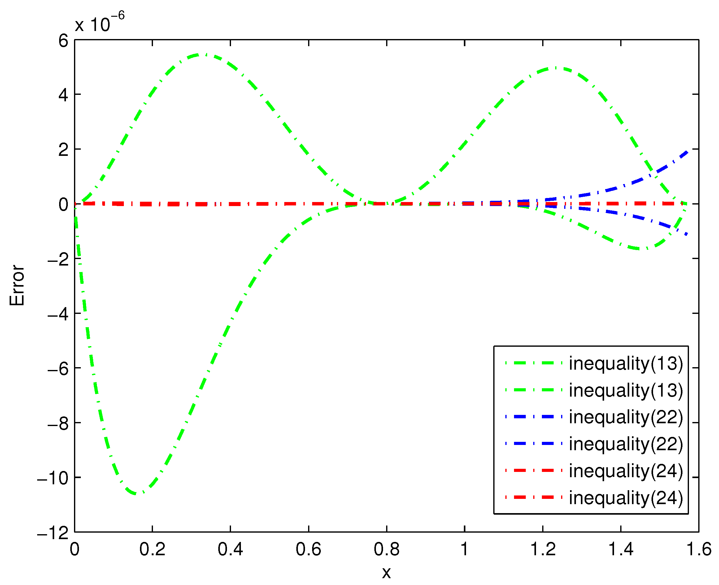
Zhang [8] (Inequality (13)) 1.0600 × 10 5 5.4563 × 10 6
Zhang [21] (Inequality (22)) 1.1234 × 10 6 1.9032 × 10 6
Results of this paper (Inequality (24))4.1030 × 10 8 2.4379 × 10 8
Table 2. Comparison of the maximum errors between cos ( x ) and the bounds for different methods.
MethodError
MaxError cos _ low MaxError cos _ upp
Sándor [18] (Inequality (16)) 2.1051 × 10 1 5.6010 × 10 2
Sándor [18] (Inequality (17)) 2.3325 × 10 1 5.6010 × 10 2
Zhang [7] (Inequality (18)) 7.2818 × 10 2 5.6010 × 10 2
Bhayo [19] (Inequality (19)) 2.3230 × 10 2 1.0599 × 10 2
Zhang [21] (Inequality (23)) 1.3987 × 10 5 2.9435 × 10 5
Results of this paper (Inequality (25))3.4330 × 10 7 2.0736 × 10 7

