Directionally Correlated Movement Can Drive Qualitative Changes in Emergent Population Distribution Patterns

Abstract

A fundamental goal of ecology is to understand the spatial distribution of species. For moving animals, their location is crucially dependent on the movement mechanisms they employ to navigate the landscape. Animals across many taxa are known to exhibit directional correlation in their movement. This work explores the effect of such directional correlation on spatial pattern formation in a model of between-population taxis (i.e., movement of each population in response to the presence of the others). A telegrapher-taxis formalism is used, which generalises a previously studied diffusion-taxis system by incorporating a parameter T, measuring the characteristic time for directional persistence. The results give general criteria for determining when changes in T will drive qualitative changes in the predictions of linear pattern formation analysis for $N\ge 2$ populations. As a specific example, the $N=2$ case is explored in detail, showing that directional correlation can cause one population to ‘chase’ the other across the landscape while maintaining a non-constant spatial distribution. Overall, this study demonstrates the importance of accounting for directional correlation in movement for understanding both quantitative and qualitative aspects of species distributions.

1. Introduction

Understanding spatial distributions of animal species is a key concern for ecology, being of fundamental importance for a wide range of applications including conservation efforts [1], quantifying biodiversity [2], and invasive species research [3,4]. For mobile animals, decisions about where to move drive their individual locations. Consequently there has been a huge amount of effort in recent years to understand the causes and consequences of animal movement [5,6,7]. However, these movement decisions have an effect not only on individuals’ locations but also on the spatial distribution of the whole population [8]. To understand this individual-to-population upscaling in a non-speculative way requires mathematical models that are built from the underlying movement processes of individuals [9]. Such models exhibit emergent phenomena on the population level that can be then quantified and related concretely to the underlying mechanisms of individual movement (e.g., [10,11]).

One recent study in this general area examines how the movement responses between individuals from $N\ge 2$ different animal populations can drive spatio-temporal distribution patterns on temporal scales whereby births and deaths are negligible [12]. This takes spatial ecology in a slightly different direction to its tradition trajectory, whereby the combination of nonlinear birth-and-death terms (a.k.a. kinetics) combine with diffusive or cross-diffusive movement to drive spatio-temporal patterns [13,14,15,16,17]. Instead, the study of [12] shows that inter-population taxis (a form of cross-diffusion) can drive a wide range of complex patterns on its own, without the need for nonlinear kinetics.

However, the study by [12] assumes that individuals move diffusively in the absence of interactions. While this may be a reasonable approximation in many cases, in reality animals will always display some directional correlation in movement [18,19], if only due to the significant energetic costs of turning [20]. For some organisms, this correlation may only persist over quite small spatio-temporal scales, in which case diffusion is a reasonable model [21,22]. However, if the spatial scale of correlation is at a similar order of magnitude to the scale over which animals move in the time between successive interactions, diffusive assumptions may be less valid [23].

Here, I address this issue of directional correlation by extending the model of [12] from a diffusion-taxis system to a telegrapher-taxis system in 1D. The telegrapher’s equation accurately models random movement with directional correlation in a 1D setting [24,25]. Moreover, it is a direct generalisation of the diffusion equation, simply requiring the introduction of a characteristic time-scale parameter, T, which is set to $T=0$ in the diffusion limit.

The aim of this study is to examine the effect of introducing $T>0$ on the linear pattern formation properties of the model in [12]. These patterning properties separate parameter space into three well-known categories [26]. First, patterns may not form at all from small non-constant perturbations of the steady state, i.e., the system is stable to such perturbations. Second, small non-constant perturbations of the steady state may grow over small times in a non-oscillatory fashion. This is classically known as a Turing instability after [27]. Third, these perturbations may both grow in magnitude and oscillate, which is sometimes known as a Turing-Hopf instability.

I give general criteria for when an increase T can cause a shift from one of these three patterning regions to another. When this shift occurs, it holds for all $T>T_{\ast }$ where $T_{\ast }$ is a threshold persistence time, which is quantified. As an example, I examine in detail the case $N=2$ in the absence of self-aggregation. Here, the diffusion-taxis model ($T=0$) can either be stable to non-constant perturbations or exhibit a Turing instability, dependent on the parameter values of the model. Furthermore, the parameter regimes where the system falls into these two patterning regions is known precisely [12]. However, the $N=2$ and $T=0$ case is never susceptible to a Turing-Hopf instability unless a self-aggregation process is in play [28]. I show that when T is increased sufficiently high, Turing-Hopf instabilities are possible without self-aggregation. Furthermore, they occur when the populations are engaged in a “pursuit-and-avoid” situation, with one population exhibiting taxis towards the other, and the latter exhibiting taxis away from the first. In contrast, for $T=0$, this pursuit-and-avoid situation is always linearly stable to non-constant perturbations.

2. The Modelling Framework and General Results

This work focusses on a system of N populations, each of fixed size (i.e., no births or deaths). Individuals from each population move on a 1D landscape as biased, correlated random walkers (i.e., those where there is both persistence in movement and bias in a particular direction). This bias depends on the density of the various populations in the system, and is represented by a taxis term up or down the density gradient of the various populations. The correlated aspect of movement is modelled using a telegrapher’s equation formalism [24,25].

Denoting by $u_i(x,t)$ the spatial probability density function of population i at time t, the study system is given by the following telegrapher-taxis equation for each population i ($i\in \{1,\dots ,N\}$)

$$\begin{array}{cc}\hfill T\frac{{\partial }^2{u}_i}{\partial t^2}+\frac{\partial u_i}{\partial t}& =d_i\frac{{\partial }^2{u}_i}{\partial x^2}-\frac{\partial }{\partial x}\left[u_i\sum _{j=1}^N{\gamma }_{ij}\frac{\partial }{\partial x}(\mathcal{K}\ast u_j)\right],\hfill \end{array}$$

(1)

where $T\ge 0$, $d_i>0$, ${\gamma }_{ij}\in \mathbb{R}$, and one can assume, without loss of generality, that the units are dimensionless and $d_1=1$. The case where $T=0$ and ${\gamma }_{ii}=0$ for all i was studied in [12], and the reader is referred there for details of the non-dimensionalisation process. The dynamics take place on a unit line segment, $[0,1]$, with periodic boundary conditions

$$\begin{array}{c}\hfill u_i(0,t)=u_i(1,t),\end{array}$$

(2)

so locations, x, live in the quotient space $[0,1]/\{0,1\}$. In Equation (1), $\mathcal{K}\left(x\right)$ is an integrable function, symmetric about $x=0$ on the domain $[0,1]/\{0,1\}$, and $\mathcal{K}\ast u_j$ is the following spatial convolution

$$\begin{array}{c}\hfill \mathcal{K}\ast u_j(x,t)={\int }_0^1\mathcal{K}(x-y)u_j(y,t)\mathrm{d}y.\end{array}$$

(3)

The inter-population taxis term, in the right-hand summand of Equation (1), can come about through different biological mechanisms. The simplest is for the organisms in population i to sense directly the gradient of population density, $\frac{\partial }{\partial x}(\mathcal{K}\ast u_j)$, a mechanism that may be valid for very small individuals such as single-celled organisms or swarming insects. However, for larger organisms, this population gradient is more likely to be observed indirectly. For example, the deposition of marks in the environment from population j (e.g., through scenting; [29,30]) may indicate the population density, $u_j$, across space. Similarly, memory of past interactions with individuals from population j can act as a proxy for sensing the population density gradient [31,32]. In [12], the authors showed how all of these biological mechanism can be modelled via the same taxis term, given in Equation (1).

The linear pattern formation properties of Equation (1) are analysed by perturbing the system about the constant steady-state solution, $u_i(x,t)=1$ for all $i,x,t$. Specifically, let $\mathbf{w}(x,t)={(u_1-1,\cdots ,u_N-1)}^{\prime }={(u_1^{\left(0\right)},\cdots ,u_N^{\left(0\right)})}^{\prime }exp(\sigma t+\mathrm{i}\kappa x)$, where $u_1^{\left(0\right)},\cdots ,u_N^{\left(0\right)}\in \mathbb{R}$, $\kappa \in {\mathbb{R}}_{\ge 0}$ and $\sigma \in \mathbb{C}$ are constants, and ${}^{\prime }$ denotes matrix transpose. By neglecting non-linear terms, Equation (1) becomes

$$\begin{array}{c}\hfill (T{\sigma }^2+\sigma )\mathbf{w}={\kappa }^{2}M\left(\kappa \right)\mathbf{w},\end{array}$$

(4)

where $M\left(\kappa \right)={\left[M_{ij}\left(\kappa \right)\right]}_{i,j}$ is an $N\times N$ matrix with

$$\begin{array}{c}\hfill M_{ij}\left(\kappa \right)=\left\{\begin{array}{cc}-d_i+{\gamma }_{ii}\widehat{\mathcal{K}}\left(\kappa \right),\hfill & \mathrm{if}i=j,\hfill \\ {\gamma }_{ij}\widehat{\mathcal{K}}\left(\kappa \right),\hfill & \mathrm{otherwise},\hfill \end{array}\right.\end{array}$$

(5)

and $\widehat{\mathcal{K}}\left(\kappa \right)$ is the Fourier transform of $\mathcal{K}\left(x\right)$ on $[0,1]/\{0,1\}$.

Let ${\lambda }_1\left(\kappa \right),\cdots ,{\lambda }_N\left(\kappa \right)$ be the eigenvalues of $M\left(\kappa \right)$ (which are not necessarily distinct). If $T=0$ then $\sigma ={\kappa }^2{\lambda }_i\left(\kappa \right)$ gives a solution to Equation (4) for some non-trivial vector $\mathbf{w}$. From the perspective of pattern formation, there are three regimes of interest. These are well-documented [26] but it is valuable to summarise them briefly, for the purposes of introducing the key concepts and nomenclature used throughout this work:

• Stable. All eigenvalues have negative real part: Re$\left({\lambda }_i\left(\kappa \right)\right)<0$ for all $i\in \{1,\cdots ,N\}$, $\kappa >0$,
• Turing instability. The dominant eigenvalue (i.e., the one with the largest real part) is positive and real, i.e., ${\mathrm{argmax}}_{{\lambda }_i\left(\kappa \right)}\left[\mathrm{Re}\left({\lambda }_i\left(\kappa \right)\right)\right]\in {\mathbb{R}}_{>0}$,
• Turing-Hopf instability. The dominant eigenvalue is not real but has positive real part, i.e., ${\mathrm{argmax}}_{{\lambda }_i\left(\kappa \right)}\left[\mathrm{Re}\left({\lambda }_i\left(\kappa \right)\right)\right]\in \{z\in \mathbb{C}:\mathrm{Re}\left(z\right)>0,z\notin \mathbb{R}\}$.

The first of these states that the linear perturbation, $\mathbf{w}(x,t)$, will decay back to the homogeneous steady state, the second that $\mathbf{w}(x,t)$ will grow at small times for certain wavenumbers, $\kappa$, in a non-oscillatory fashion, and the third that $\mathbf{w}(x,t)$ will grow and oscillate at small times. These regimes give an indication for the pattern formation properties of the system. In the Stable region, the expectation is that spatial patterns do not form. In the Turing instability region, stationary patterns are predicted to form, which are fixed over time. If there is a Turing-Hopf instability, patterns that are in perpetual flux are expected to emerge. However, it is important to note that these are merely predictions, arising from a linearisation of the system, and that it is possible for the non-linear terms to cause different pattern formation properties asymptotically.

The main aim of this work is to examine how the demarcation into the above three regimes changes as T is increased from 0. When $T>0$, for each $i\in \{1,\cdots ,N\}$, there are up to two values of $\sigma$ such that $T{\sigma }^2+\sigma ={\kappa }^2{\lambda }_i\left(\kappa \right)$. Thus I define

$$\begin{array}{c}\hfill {\sigma }_i^{\pm }(\kappa ,T)=\frac{-1\pm \sqrt{1+4T{\kappa }^2{\lambda }_i\left(\kappa \right)}}{2T},\end{array}$$

(6)

for each $i\in \{1,\cdots ,N\}$, and note that ${\sigma }_i^{\pm }(\kappa ,T)$ solves Equation (4) for each i. The main results from this work are given in the following three theorems.

Theorem 1.

In the case where the system is linearly stable for $T=0$ (i.e., Re$\left({\lambda }_i\left(\kappa \right)\right)<0$ for all $i\in \{1,\cdots ,N\}$, $\kappa >0$) one of two situations can occur:

1 

If ${\lambda }_i\left(\kappa \right)\in \mathbb{R}$ for all $i,\kappa$, then Re$\left({\sigma }_i^{\pm }(\kappa ,T)\right)<0$ for all $i,\kappa ,T$, so the system stays in the Stable regime for all $T>0$.

2 

If there exist i and κ such that ${\lambda }_i\left(\kappa \right)\notin \mathbb{R}$ then there exists some $T_{\ast }>0$ such that for all $T>T_{\ast }$, there is a Turing-Hopf instability. In other words, for this value of i and κ, ${\mathit{argmax}}_{{\sigma }_i(\kappa ,T)}[\mathit{Re}\left({\sigma }_i(\kappa ,T)\right]\in \{z\in \mathbb{C}:\mathit{Re}\left(z\right)>0,z\notin \mathbb{R}\}$ for all $T>T_{\ast }$. Furthermore, $T_{\ast }$ is the minimum $T>0$ such that there exist $i,\kappa$ with Re$\left(\sqrt{1+4T{\kappa }^2{\lambda }_i\left(\kappa \right)}\right)>1$.

Proof. 

For part (1), if ${\lambda }_i\left(\kappa \right)\in \mathbb{R}$ for all $i,\kappa$ then, since Re$\left({\lambda }_i\left(\kappa \right)\right)<0$, the inequality $1+4T{\kappa }^2{\lambda }_i\left(\kappa \right)<1$ holds, so Re$\left({\sigma }_i^{\pm }(\kappa ,T)\right)<0$ for all $i,\kappa ,T$.

For part (2), let $i\in \{1,\cdots ,N\}$ and $\kappa >0$ such that ${\lambda }_i\left(\kappa \right)\notin \mathbb{R}$. Assume, without loss of generality, that Im$\left({\lambda }_i\left(\kappa \right)\right)>0$ (otherwise, pick the complex conjugate of ${\lambda }_i\left(\kappa \right)$). Then if Re$\left(\sqrt{1+4T{\kappa }^2{\lambda }_i\left(\kappa \right)}\right)>1$, the inequality Re$\left({\sigma }_i^{+}(\kappa ,T)\right)>0$ holds, so that there is a Turing-Hopf instability.

I now show that if T is arbitrarily large, the criterion Re$\left(\sqrt{1+4T{\kappa }^2{\lambda }_i\left(\kappa \right)}\right)>1$ is always satisfied. Here,

$$\begin{array}{c}\hfill \mathrm{Re}\left(\sqrt{1+4T{\kappa }^2{\lambda }_i\left(\kappa \right)}\right)\approx \mathrm{Re}\left(\sqrt{4T{\kappa }^2{\lambda }_i\left(\kappa \right)}\right).\end{array}$$

(7)

Now, arg$\left(\sqrt{4T{\kappa }^2{\lambda }_i\left(\kappa \right)}\right)=$arg$\left({\lambda }_i\left(\kappa \right)\right)/2$. Since Im$\left({\lambda }_i\left(\kappa \right)\right)>0$ and Re$\left({\lambda }_i\left(\kappa \right)\right)<0$, the following holds

$$\begin{array}{c}\hfill \pi /2<\arg \left({\lambda }_i\left(\kappa \right)\right)<\pi .\end{array}$$

(8)

Therefore

$$0<\arg \left(\sqrt{4T{\kappa }^2{\lambda }_i\left(\kappa \right)}\right)<\pi /2,$$

so that Re($\sqrt{4T{\kappa }^2{\lambda }_i\left(\kappa \right)})>0$. Hence Re$\left(\sqrt{1+4T{\kappa }^2{\lambda }_i\left(\kappa \right)}\right)>0$ whenever T is sufficiently large. Furthermore, Re$\left(\sqrt{1+4T{\kappa }^2{\lambda }_i\left(\kappa \right)}\right)\to \infty$ as $T\to \infty$, so there exists some $T_{\ast }^{i,\kappa }$ such that Re$\left(\sqrt{1+4T{\kappa }^2{\lambda }_i\left(\kappa \right)}\right)>1$ for all $T>T_{\ast }^{i,\kappa }$. There may be more than one $j\in \{1,\cdots ,N\}$ and $\kappa >0$ such that ${\lambda }_j\left(\kappa \right)\notin \mathbb{R}$. Thus let $T_{\ast }$ be the minimum of $T_{\ast }^{j,\kappa }$ over such j and all $\kappa$. Then $T_{\ast }$ satisfies the requirements of the theorem. □

Theorem 2.

Consider the Turing instability case for $T=0$ (i.e., ${\mathit{argmax}}_{{\lambda }_i\left(\kappa \right)}[\mathit{Re}\left({\lambda }_i\left(\kappa \right)\right]\in {\mathbb{R}}_{>0}$). For a given κ, let ${\lambda }_i\left(\kappa \right)$ be the dominant eigenvalue of $M\left(\kappa \right)$. Then one of two situations can occur:

1 

If Re$\left(\sqrt{1+4{\kappa }^{2}T{\lambda }_j\left(\kappa \right)}\right)\le \sqrt{1+4{\kappa }^{2}T{\lambda }_i\left(\kappa \right)}$ for all j then there is a Turing instability at wavenumber κ and persistence time T.

2 

If there is some j such that Re$\left(\sqrt{1+4{\kappa }^{2}T{\lambda }_j\left(\kappa \right)}\right)>\sqrt{1+4{\kappa }^{2}T{\lambda }_i\left(\kappa \right)}$ then there is a Turing-Hopf instability at wavenumber κ and persistence time T. Let $T_{\ast }$ be the minimum $T>0$ such that Re$\left(\sqrt{1+4{\kappa }^{2}T{\lambda }_j\left(\kappa \right)}\right)>\sqrt{1+4{\kappa }^{2}T{\lambda }_i\left(\kappa \right)}$ for some j. Then there is a Turing-Hopf instability for all $T>T_{\ast }$.

Proof. 

For part (1), let $\kappa ,T>0$. If Re$\left(\sqrt{1+4{\kappa }^{2}T{\lambda }_j\left(\kappa \right)}\right)\le \sqrt{1+4{\kappa }^{2}T{\lambda }_i\left(\kappa \right)}$ for all j then ${\sigma }_i^{+}(\kappa ,T)$ is the dominant eigenvalue. Since ${\lambda }_i\left(\kappa \right)\in {\mathbb{R}}_{>0}$, $\sqrt{1+4{\kappa }^{2}T{\lambda }_i\left(\kappa \right)}\in {\mathbb{R}}_{>1}$ so ${\sigma }_i^{+}(\kappa ,T)\in {\mathbb{R}}_{>0}$ so there is a Turing instability for these values of T and $\kappa$.

For part (2), suppose there exist $j,T,\kappa$ with Re$\left(\sqrt{1+4{\kappa }^{2}T{\lambda }_j\left(\kappa \right)}\right)>\sqrt{1+4{\kappa }^{2}T{\lambda }_i\left(\kappa \right)}$ and suppose Re$\left(\sqrt{1+4{\kappa }^{2}T{\lambda }_j\left(\kappa \right)}\right)\ge \mathrm{Re}\left(\sqrt{1+4{\kappa }^{2}T{\lambda }_k\left(\kappa \right)}\right)$ for all k. Then ${\sigma }_j^{+}(\kappa ,T)$ is the dominant eigenvalue. It is necessary to show that ${\sigma }_j^{+}(\kappa ,T)$ is not real. Therefore, for a contradiction, suppose $\sqrt{1+4{\kappa }^{2}T{\lambda }_j\left(\kappa \right)}\in \mathbb{R}$. Then ${\lambda }_j\left(\kappa \right)\in \mathbb{R}$. However, ${\lambda }_j\left(\kappa \right)\le {\lambda }_i\left(\kappa \right)$, since ${\lambda }_i\left(\kappa \right)$ is the dominant eigenvalue of $M\left(\kappa \right)$, so $\sqrt{1+4{\kappa }^{2}T{\lambda }_j\left(\kappa \right)}\le \sqrt{1+4{\kappa }^{2}T{\lambda }_i\left(\kappa \right)}$, which contradicts the assumption. Hence ${\sigma }_j^{+}(\kappa ,T)\notin \mathbb{R}$ so there is a Turing-Hopf instability for these values of T and $\kappa$. □

Corollary. If there is some j such that Re$\left(\sqrt{{\lambda }_j\left(\kappa \right)}\right)>\sqrt{{\lambda }_i\left(\kappa \right)}$ then there is a Turing-Hopf instability at wavenumber $\kappa$ for sufficiently large T.

Theorem 3.

Consider the case where there is a Turing-Hopf instability for $T=0$. Then there is a Turing-Hopf instability for all $T>0$.

Proof. 

Let i be such that ${\lambda }_i\left(\kappa \right)$ is the dominant eigenvalue of $M\left(\kappa \right)$ for some $\kappa$ where there is a Turing-Hopf instability for $T=0$. Assume, without loss of generality, that Im$\left({\lambda }_i\left(\kappa \right)\right)>0$ (otherwise choose the complex conjugate of ${\lambda }_i\left(\kappa \right)$). Since Re$\left({\lambda }_i\left(\kappa \right)\right)>0$, the inequality Re$(1+4T{\kappa }^2{\lambda }_i\left(\kappa \right))>1$ holds, so $\sqrt{\mathrm{Re}(1+4T{\kappa }^2{\lambda }_i\left(\kappa \right))}>1$. Since $1+4T{\kappa }^2{\lambda }_i\left(\kappa \right)$ has positive real and imaginary part, $\sqrt{\mathrm{Re}(1+4T{\kappa }^2{\lambda }_i\left(\kappa \right))}<\mathrm{Re}\left(\sqrt{1+4T{\kappa }^2{\lambda }_i\left(\kappa \right)}\right)$. The latter follows from the following general calculation for $r>0$ and $0<\theta <\pi /2$

$$\begin{array}{c}\hfill \sqrt{\mathrm{Re}\left(r{\mathrm{e}}^{\mathrm{i}\theta }\right)}=\sqrt{r}\sqrt{cos\left(\theta \right)}<\sqrt{r}\sqrt{\frac{cos\left(\theta \right)+1}{2}}=\sqrt{r}cos\left(\frac{\theta }{2}\right)=\mathrm{Re}\left(\sqrt{r{\mathrm{e}}^{\mathrm{i}\theta }}\right).\end{array}$$

(9)

The inequality in (9) requires $0<cos\left(\theta \right)<1$, which follows from $0<\theta <\pi /2$.

It follows that $\mathrm{Re}\left(\sqrt{1+4T\kappa {\lambda }_i\left(\kappa \right)}\right)>1$, and thus from Equation (6) that Re$\left({\sigma }_i^{+}(\kappa ,T)\right)>0$ for all $T>0$. To show that this is within the Turing-Hopf instability region, it is necessary to check that there does not exist j such that both ${\sigma }_j^{+}(\kappa ,T)\in {\mathbb{R}}_{>0}$ and ${\sigma }_j^{+}(\kappa ,T)>\mathrm{Re}\left({\sigma }_i^{+}(\kappa ,T)\right)$, since otherwise this is the Turing instability region. For a contradiction, suppose such a ${\sigma }_j^{+}(\kappa ,T)$ exists. Then

$$\begin{array}{c}\hfill \sqrt{1+4T{\kappa }^2{\lambda }_j\left(\kappa \right)}>\mathrm{Re}\left(\sqrt{1+4T{\kappa }^2{\lambda }_i\left(\kappa \right)}\right)>\sqrt{\mathrm{Re}(1+4T{\kappa }^2{\lambda }_i\left(\kappa \right))}\end{array}$$

(10)

so $1+4T{\kappa }^2{\lambda }_j\left(\kappa \right)>\mathrm{Re}(1+4T{\kappa }^2{\lambda }_i\left(\kappa \right))$ so ${\lambda }_j\left(\kappa \right)>\mathrm{Re}\left({\lambda }_i\left(\kappa \right)\right)$, which contradicts the fact that ${\lambda }_i\left(\kappa \right)$ is the dominant eigenvalue for the $T=0$ case. □

3. The Case of Two Interacting Populations ($\mathit{N}=\mathbf{2}$)

In this section, I look in detail at the specific example where $N=2$ and ${\gamma }_{ii}=0$ for all $i\in \{1,\cdots ,N\}$, to show how persistent movement can drive qualitative changes in pattern formation properties even in this simple situation. In the case $T=0$ (studied by [12]), the following holds

$$\begin{array}{c}\hfill {\lambda }_{\pm }\left(\kappa \right)=\frac{-(1+d_2)\pm \sqrt{{(1-d_2)}^2+4{\gamma }_{12}{\gamma }_{21}{\widehat{\mathcal{K}}}^2\left(\kappa \right)}}{2},\end{array}$$

(11)

and it follows that the system for $T=0$ is linearly stable to wave perturbations whenever ${\gamma }_{12}{\gamma }_{21}<d_2$. When ${\gamma }_{12}{\gamma }_{21}>d_2$, the system can have a Turing instability, and always does in the limit $\widehat{\mathcal{K}}\left(\kappa \right)\to 1$, where the spatial averaging given by $\mathcal{K}$ is arbitrarily small. The system never exhibits a Turing-Hopf instability for $T=0$ [12].

In the Turing instability case for $T=0$, both the eigenvalues are real, so the conditions of Theorem 2, part 2, are met. Thus there is a Turing instability for all $T>0$. The case where ${\gamma }_{12}{\gamma }_{21}<d_2$, however, is more interesting. Here, Theorem 1 states that a Turing-Hopf instability will occur for sufficiently large T as long as ${\lambda }_{\pm }\left(\kappa \right)\notin \mathbb{R}$, that is

$$\begin{array}{c}\hfill {(1-d_2)}^2+4{\gamma }_{12}{\gamma }_{21}{\widehat{\mathcal{K}}}^2\left(\kappa \right)<0.\end{array}$$

(12)

The first thing to notice about the condition given by (12) is that ${\gamma }_{12}$ and ${\gamma }_{21}$ need to be of opposite signs. This means that one population tends to advect up the density gradient of the other, while the second population retreats down the gradient of the first. This is termed a ‘pursuit-and-avoid’ situation in [12]. In this situation, for $T=0$, no patterns form: the populations each settle to a steady-state distribution whereby they are uniformly distributed on the terrain. However, if $T_{\ast }$ is defined to be the minimum positive real number such that there exists $\kappa >0$ with Re$\left(\sqrt{1+4T{\kappa }^2{\lambda }_{+}\left(\kappa \right)}\right)>1$, then Theorem 1 implies there is a Turing-Hopf instability whenever $T>T_{\ast }$.

To understand how $T_{\ast }$ depends on the parameters, I fix $d_2=1$ and set $\gamma =+\sqrt{-{\gamma }_{12}{\gamma }_{21}}$. (Notice that $\gamma \in {\mathbb{R}}_{>0}$ since ${\gamma }_{12}$ and ${\gamma }_{21}$ are of opposite signs.) It is also necessary to pick a particular functional form for $\mathcal{K}\left(x\right)$. This is a slightly delicate matter as it is not necessarily the case that the pattern formation problem is well-posed for an arbitrary $\mathcal{K}\left(x\right)$. For example, if $\mathcal{K}\left(x\right)=\delta \left(x\right)$ is used, where $\delta \left(x\right)$ is the Dirac delta function, then, by Equation (6), the dominant eigenvalue is

$$\begin{array}{c}\hfill {\sigma }_i^{+}(\kappa ,T)=\frac{-1+\sqrt{1-4T{\kappa }^2+4T\mathrm{i}{\kappa }^2\gamma }}{2T}.\end{array}$$

(13)

If T is fixed and $\kappa$ is arbitrarily large, then Re$\left({\sigma }_i^{+}(\kappa ,T)\right)\approx \kappa$Re$(\sqrt{-1+\mathrm{i}\gamma }/\sqrt{T})\to \infty$ as $\kappa \to \infty$. Hence patterns can form for arbitrarily high wavenumbers, meaning the pattern formation problem is ill-posed.

However, suppose instead that

$$\begin{array}{c}\hfill \mathcal{K}\left(x\right)=\left\{\begin{array}{cc}\frac{exp\left(-\frac{x^2}{{\sigma }^2}\right)}{\sigma \sqrt{\pi }erf\left(\frac{1}{2\sigma }\right)},\hfill & \mathrm{if}-1/2<x<1/2\hfill \\ 0,\hfill & \mathrm{otherwise},\hfill \end{array}\right.\end{array}$$

(14)

for some $\sigma >0$, so that

$$\begin{array}{c}\hfill \widehat{\mathcal{K}}\left(\kappa \right)=\frac{\mathrm{erf}\left(\frac{1}{2\sigma }-\frac{\mathrm{i}\kappa \sigma }{2}\right)+\mathrm{erf}\left(\frac{1}{2\sigma }+\frac{\mathrm{i}\kappa \sigma }{2}\right)}{2\mathrm{erf}\left(\frac{1}{2\sigma }\right)}exp\left(\frac{-{\kappa }^2{\sigma }^2}{4}\right).\end{array}$$

(15)

The case of interest is where $\sigma$ is small, in which case the following approximation can be made

$$\begin{array}{c}\hfill \widehat{\mathcal{K}}\left(\kappa \right)\approx exp\left(\frac{-{\kappa }^2{\sigma }^2}{4}\right).\end{array}$$

(16)

Then Equation (6) gives

$$\begin{array}{c}\hfill {\sigma }_i^{+}(\kappa ,T)=\frac{-1+\sqrt{1-4T{\kappa }^2+4T\mathrm{i}\gamma {\kappa }^{2}exp(-{\kappa }^2{\sigma }^2/4)}}{2T}.\end{array}$$

(17)

Now, notice that if T is fixed and $\kappa$ is arbitrarily large, then

$$\begin{array}{c}\hfill \mathrm{Re}\left({\sigma }_i^{+}(\kappa ,T)\right)\approx \kappa \mathrm{Re}\left(\frac{\sqrt{-1+\mathrm{i}\gamma exp(-{\kappa }^2{\sigma }^2/4)}}{\sqrt{T}}\right)\to 0,\end{array}$$

(18)

as $\kappa \to \infty$. Therefore, with the Gaussian averaging kernel from Equation (14), the pattern formation problem is well-posed, in the sense that patterns cannot form at arbitrarily high wavenumbers.

By Theorem 1, there is some $T_{\ast }$ such that there is a Turing-Hopf instability for all $T>T_{\ast }$. Furthermore, this Theorem states that $T_{\ast }$ is the minimum T such that the following holds for some $\kappa$

$$\begin{array}{c}\hfill f\left(\kappa \right):=\mathit{Re}\left[\sqrt{1-4T{\kappa }^2+4T\mathrm{i}\gamma {\kappa }^{2}exp(-{\kappa }^2{\sigma }^2/4)}\right]>1.\end{array}$$

(19)

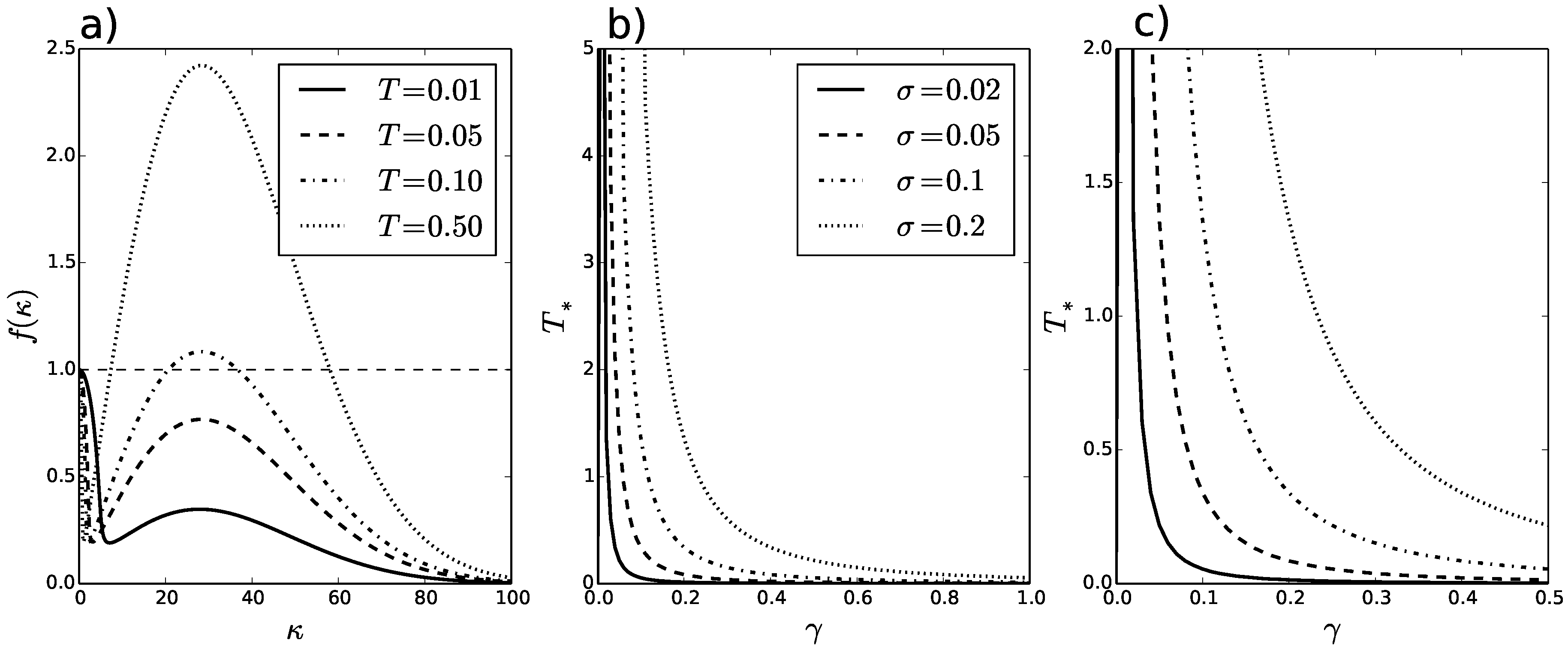
In Figure 1a, $f\left(\kappa \right)$ is plotted against $\kappa$ for $\gamma =0.2$, $\sigma =0.05$, and varying values of T. This reveals that T not only affects whether patterns form, but the range of wavenumbers for which patterns may form. In this example, there is a Turing-Hopf bifurcation for value of $T=T_{\ast }$ somewhere between $T=0.05$ and $T=0.1$.

The precise values of $T_{\ast }$ for a range of $\gamma$- and $\sigma$-values are plotted in Figure 1b,c. The $\gamma$ parameter encodes the strength of attraction/avoidance. Figure 1b,c shows that $T_{\ast }$ decays for increasing $\gamma$ and grows with the width of spatial averaging, $\sigma$.

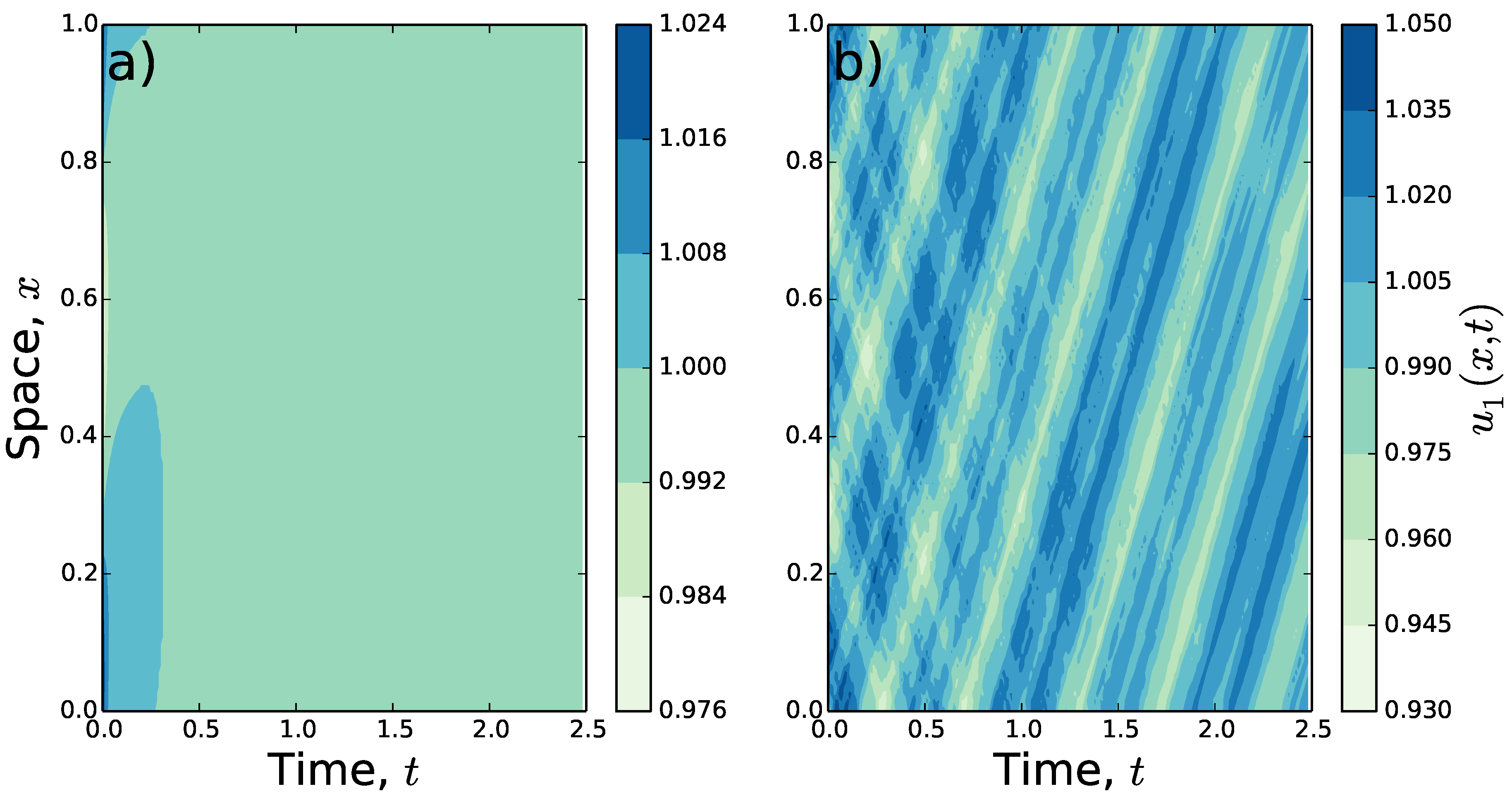
To understand the qualitative properties of the patterns that emerge from increasing $T_{\ast }$ past the Turing-Hopf bifurcation point, the system in Equations (1)–(3) is solved numerically, with $N=2$, $d_2=1$, $\gamma =+\sqrt{-{\gamma }_{12}{\gamma }_{21}}$, and the Gaussian spatial averaging from Equation (14). In Figure 2, the results of these numerics are shown for certain values of $\gamma$, $\sigma$ and T. Here, rather than decaying to the homogeneous steady state ($T=0$), for higher T the populations move across the landscape while maintaining a non-constant population distribution.

4. Discussion

This study examines a telegrapher-taxis system of N populations to demonstrate how directional correlation can drive pattern formation in systems of between-population taxis. General criteria are given for switches in pattern formation regime driven by directional correlation and the $N=2$ case is examined in detail. These results demonstrate the importance of considering directional correlation when seeking to understanding the spatio-temporal population distributions of moving organisms. As our ability to capture data on animal movement is becoming increasingly sophisticated, better understanding of how the details of animal movement can affect population dynamics is becoming an ever-more pertinent question [6], with implications for a diverse range of ecological areas such as connectivity dynamics [33] and conservation [34].

The model of [12], on which the present model is based, is closely related to aggregation and chemotaxis models inspired by cell biology [35,36,37,38]. Although many such models only examine a single population, there are various examples of two-population models [28,39], and some that incorporate an arbitrary number of populations [40,41]. In the latter examples, the diffusion-taxis equations are coupled via interactions with a diffusive chemical, different to the model studied here. While cells lack the momentum of much larger organisms, directional correlation is known to be a factor in the movement of cells in certain circumstances [42,43,44]. Therefore the results presented here suggest that it is worth exploring how directional correlation may affect the pattern formation properties of such aggregation and chemotaxis models.

Here, ecosystems are modelled on a constrained timescale whereby births and deaths are negligible. However, it would be valuable to extend the model presented here to incorporate such effects, via competition and/or predation terms (i.e., kinetics), and so explore the effect of directional persistence over longer timescales. Adding directional persistence to models that incorporate kinetics is non-trivial, though, and does not simply involve adding a second temporal derivative to a reaction-diffusion-taxis model [45].

Nonetheless, building such a system of reaction-telegrapher-taxis equations would enable connection with cross-diffusion models (e.g., [16,17,46,47]). These are generalisations of reaction-diffusion systems, whereby terms are added that allow for motion driven by the presence of foreign populations. These terms include, but are not limited to, the taxis terms observed in the model from Equation (1). However, incorporating directional correlation via a telegrapher’s term into a cross-diffusive setting is much rarer (but see [48]) and the pattern formation properties of such systems are not well-explored. Given the results presented here, it may be interesting to extend cross-diffusive models in this way, to show how directional correlation may affect pattern formation in such models.

In summary, the simple but general results shown here demonstrate that directional correlation of individuals’ movement can have a great effect on the spatio-temporal distribution of species. While I have demonstrated this in a model of ecosystems relevant over relatively short timescales, where births and deaths are minimal, it highlights a general principle that is little-studied and may have much wider implications.