1. Introduction
The large-scale neural network models in computational neuroscience have become familiar. The classical description of these (excitatory-inhibitory) neural network models is based on the deterministic/stochastic system. One of the most common models is known as the noisy leaky integrate-and-fire (NLIF) neuron model in which the behavior of the whole population of neurons is encoded in a stochastic differential equation (SDE) for the time evolution of membrane potential of a single neuron representative of the network. The dynamics of a single neuron is given by ([
1,
2,
3,
4,
5,
6])
where
represents the membrane potential of a single neuron and
is the time relaxation of the membrane potential in the absence of any communication. The communication of a single neuron with the network is modeled by the synaptic input current,
The form of
is a stochastic process, given by ([
7])
Here, each spike is treated as a delta function, and if a spike occurs at time
it is denoted by
The terms
and
in above equation represent the time of
mth-spike receiving from
nth-presynaptic neuron for excitatory and inhibitory neurons, respectively. Moreover, the terms
and
are the total number of presynaptic neurons, where
and
are the strength of the synapses for excitatory and inhibitory neurons, respectively. Since the above form of synaptic input current is the discrete Poisson process, it becomes very difficult for further investigation. In addition, the researchers have used the diffusion approximation in which the synaptic input current
is approximated by a continuous in time Ornstein-Uhlenbeck-type stochastic process as given by
Initially, it is assumed that every neuron generates spikes according to a stationary Poisson process with constant probability of generating a spike per unit time and it is also assumed that all these processes are independent between neurons, because of these assumptions, the mean value of the current, indicated by , is given by and its variance, Here, we have to depict the likelihood of firing per unit time of the Poissonian spike train r and it is thus recognized as the firing rate, which should be computed as where is the mean firing rate of the network. On the other side, is the standard Brownian motion in above equation.
The next important factor in the modeling is that the neurons generate a spike only when its membrane potential arrives at a certain voltage, known as threshold and instantly reset toward a resetting potential and sends a signal over the network.
Comprising the continuous form of
in SDE model (1), we obtain
where
We suppose that the voltage of a neuron arrives at threshold level at time
, i.e.,
and after that the voltage arrives suddenly at resting potential, i.e.,
Furthermore, one can write the associated FPE with source term by using Ito’s rule [
8], for the evolution of probability density function
of finding neurons at a voltage
with time (
)
where
and
is the mean firing rate of the network which is computed as the flux of neuron at the firing voltage. The source term of the Equation (2) comes from the fact that when the neurons generate spikes and send the signals over the network, their voltage immediately reset to the reset potential
At the relaxation time, no neuron have the firing voltage, for this reason, the initial and boundary conditions are given by
We can easily verify the conservation of the total number of neurons in above equation. For this purpose, we need to describe the mean firing rate for the network. Since the mean firing rate is the flux of neurons at , the value of is given by Integrating (3) across the voltage domain and using the above boundary conditions, we obtain the required condition.
Equation (2) represents the evolution of probability density function and therefore
If we translate the new voltage variable by considering then we have and diffusion coefficient is of the form
In [
8], the authors provide theoretical and numerical analysis using finite difference approximation. For the references of mathematical aspects of nonlinear NLIF models, we refer [
9,
10,
11,
12,
13]. We are concern about finding the value of the unknown
using alternative approach. The problem (2)–(4) cannot be solved analytically, because of its complexity arising from nonlinearity and having a source term [
14,
15,
16]. Therefore, numerical methods are generally used, for example, finite difference method (FDM) is used to find the approximate solution of the governing equation [
8]. However, FDM has some disadvantages, for instance, the singularity in the delta source term, as in the above mentioned equation, makes the solution divergent. In order to use the FDM appropriately, the governing equation must be modified, due to the fact that the procedure becomes complicated.
Hence, in the present work, we propose a formulation based on finite element approximation to find the solution of governing equation. FEM is one of the powerful numerical methods for the solutions of problems that describe the real-life situations. Moreover, the characteristics of FEM tackle the singularity problem in an effective manner [
17,
18,
19,
20,
21,
22,
23,
24,
25,
26,
27]. The applicability of FEM regarding this model problem is demonstrated in the final section.
Description of the present paper is as follows: We consider the NLIF model described by Equations (2) and (3). In
Section 2, we develop the numerical approximation based on the finite element approach. The analysis for the stability is provided in
Section 3. We report some numerical examples from [
8] and discuss the solution behavior graphically in
Section 4. In the last section, we conclude the work done in this research article.
Preliminaries
Here, we state some basic definitions and auxiliary results, which will be used throughout the manuscript. As we are studying a nonlinear version of the FPE, we start with the notion of weak solution.
Definition 1. We say that a pair of non-negative functionswithis a weak solution of (2) and (3) if for any test functionsuch that, we have Here, the space
, refers to the space of functions such that
is integrable in
, while
corresponds to the space of bounded functions in
. The set of infinitely differentiable functions in
is denoted by
used as test functions in the notion of weak solution. The blow-up of solution and a priori estimates are given in [
8]. We here just state the results.
Theorem 1. (Blow-up) Assume that the drift and diffusion coefficients satisfyfor alland all, and let us consider the average-excitatory network where. Choose. If the initial data is concentrated enough around, in the sense thatis close enough to, then there are no global-in-time weak solutions to (2)–(4). Lemma 1 (A priori estimates).
Assumeon the drift and diffusion coefficients and thatis a global-in-time solution of (2)–(4) in the sense of Definition 1 fast decaying at, then the following a priori estimates hold for all:
IfthenMoreover, if in addition a is constant, then
In a latest work [
8], it was demonstrated that the problem (2)–(4) can produce a finite time blow-up solution for excitatory networks
when the initial data is concentrated near sufficient to the threshold voltage. This result was obtained by giving no information about the behavior at the blow-up time. In a recent work [
12], we state the theorem gives a characterization of this blow-up time when it occurs for
Theorem 2. Letbe a non-negativefunction such thatand There exist a classical solution of (2)–(4) in the time interval with
The maximal existence time can be characterized as Moreover, whenwe have thatwhile forthere exist classical solutions which blow up at a finite timeand consequently have diverging mean firing rate as
We now state the main result on steady states from [
8].
Theorem 3. Let,with.
Under either the conditionsand, or the condition, then there exists at least one steady state solution to (2)–(4).
If bothandhold, then there are at least two steady states to solution to (2)–(4).
There is no steady state to (2)–(4) under the high connectivity condition’
2. Finite Element Approximation
We construct the numerical approximation of the problem given in (2) and (3) in two ways: First we use FEM for space discretization that provides a system of ordinary differential equations, which is then solved by Euler’s backward difference for time. Spatial discretization involves the construction of a weak formulation of problem over a given domain
with specified boundary conditions at
and
Weak formulation of the problem (2) and (3) is obtained by multiplying the equation with some test function
and integrating over
,
In the present study, the mean firing rate
is approximated by using backward FDM. Performing the integration by parts in above equation, we get the following equation:
This resulting integral (8) is called weak formulation because it allows approximate function with less continuity (or differentiability) than the strong form given in Equation (2). Once we obtained the weak formulation, next step is to discretize the weak form for the easy representation and to capture the local effects more precisely. Weak form discretization consists of dividing the entire domain into set of elements, then developing the finite element model by seeking the approximation of a solution over a typical element. This discretization is tackled by taking
n non-overlapping elements say
for
with step size
h given by:
The unknown function
must be approximated in a manner so that continuity or differentiability demands by weak formulation can be met. Since the weak formulation contains the first order derivative of
any function with non-zero first derivative would be a candidate for approximation. Thus, semi discretization consists of finding
where
are the nodal values and
are the basis functions given by
There are many choices of weight function
to be used. Particular choice for the weight function
in Galerkin approach is the same as the choice of basis function
Thus, substituting weight function
and approximation for the solution defined by Equation (10) in weak formulation obtained in Equation (9) leads to the following equation:
On simplification of the above, we get as follows
Solving Equation (12), we get the system of ordinary differential equations for
which can be expressed in matrix notation given by
where
By assembling the contribution from all elements, we get the following system for the global nodal vector
on the entire domain
where
f is the column vector with all entries are zero except at reset potential
Ordinary differential Equation (14) requires implicit and stable time-stepping method to avoid extremely small time-step. Firstly we discretize the time domain
into
m subintervals with time step
We use the Euler’s backward difference in time and get the following system from Equation (14):
this algebraic system (15) can be solved for
4. Numerical Experiments
In this section, we present some numerical examples to demonstrate the behavior of the solutions of the nonlinear NLIF model. The performance of the developed scheme is tested by comparing our results with the existing scheme in the literature. Consider the system (2) and (3) with initial data as follows
where change in mean
and variance
describe different scenario of a solution. We notice that the behavior of the solution depends upon the value of excitatory (
) and inhibitory
average network. First we take constant diffusion coefficient
and find the effect on solution with change in value of
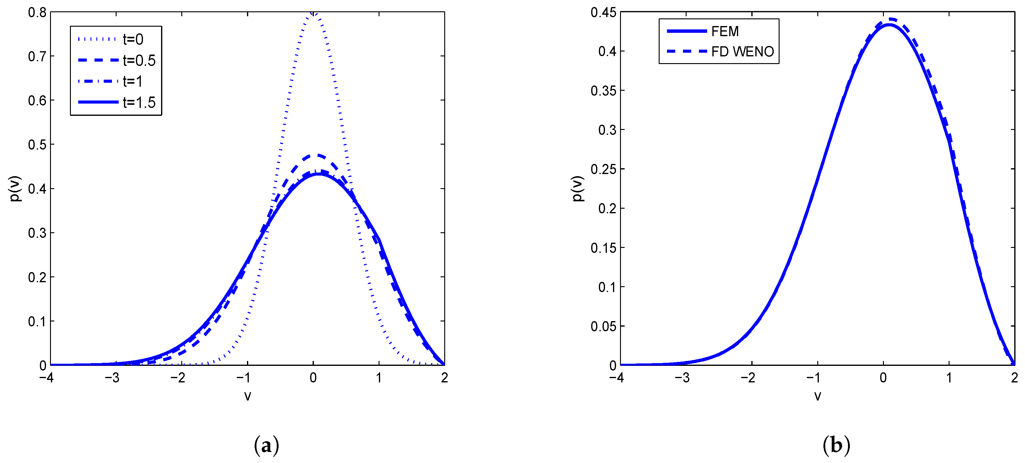
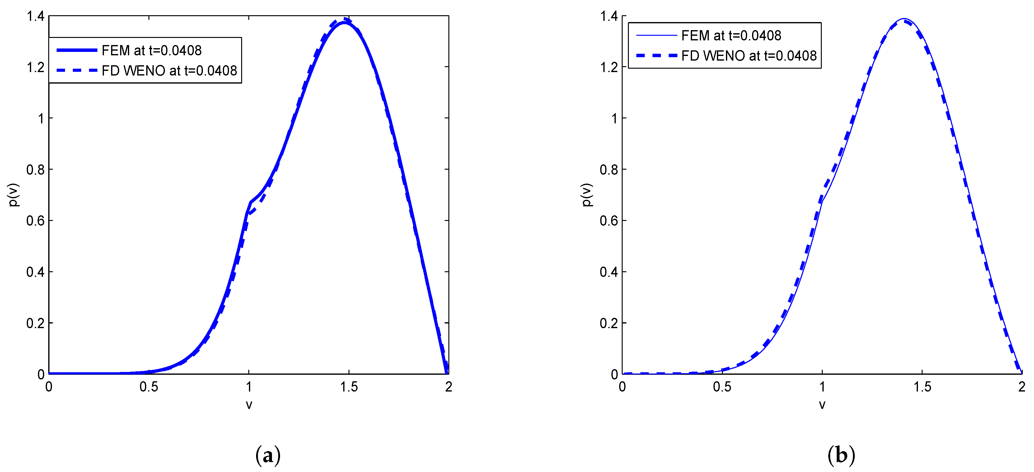
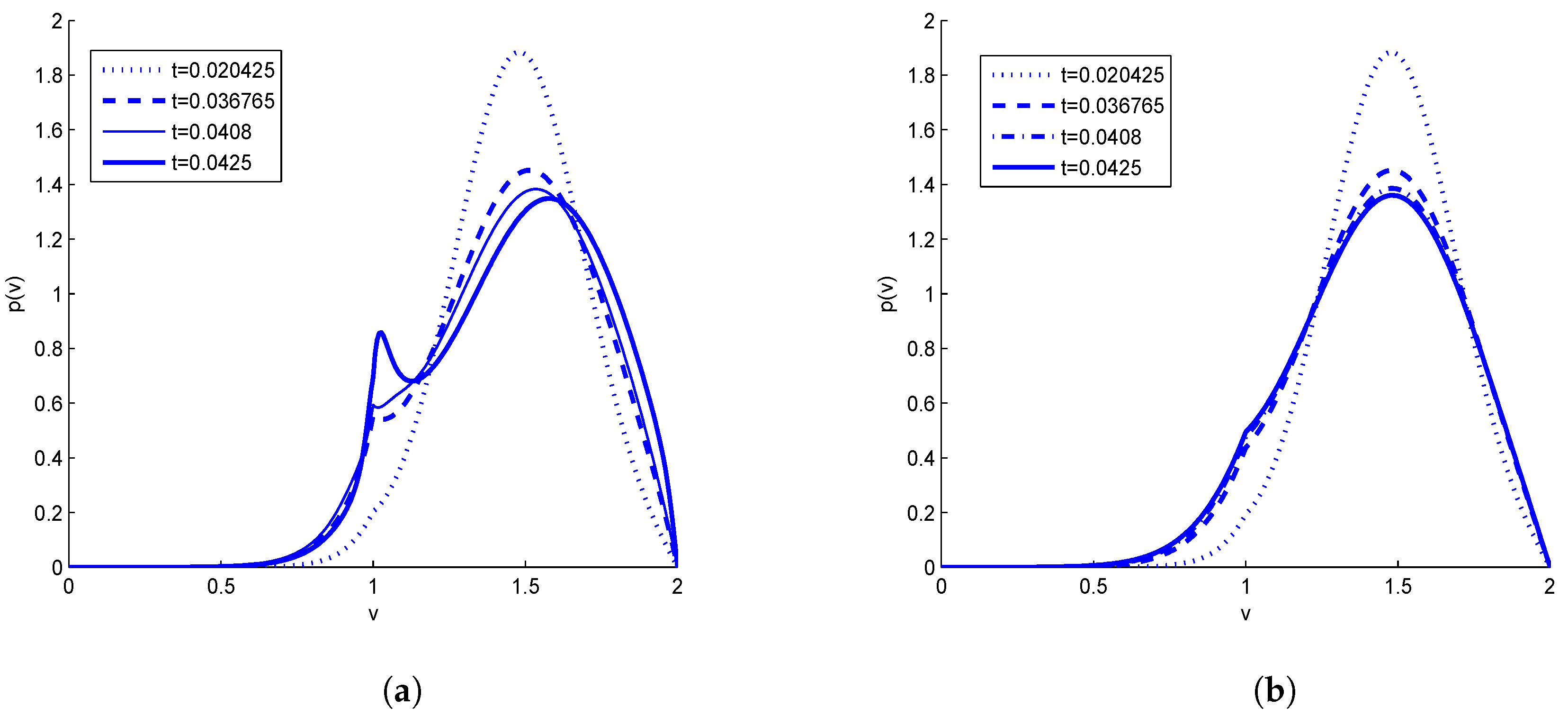
In
Figure 1a, we find that after some time the solution
goes to steady state by taking excitatory case i.e.,
small enough.
The approximate solution
for
at different time levels
is plotted in
Figure 1 with a reset potential
From
Figure 1a, we see that height of impulse decreases as time increases and after some time it reaches a steady state. In
Figure 1b, we perform numerical approximation based upon FEM and compare the results obtained in [
8] at a final time
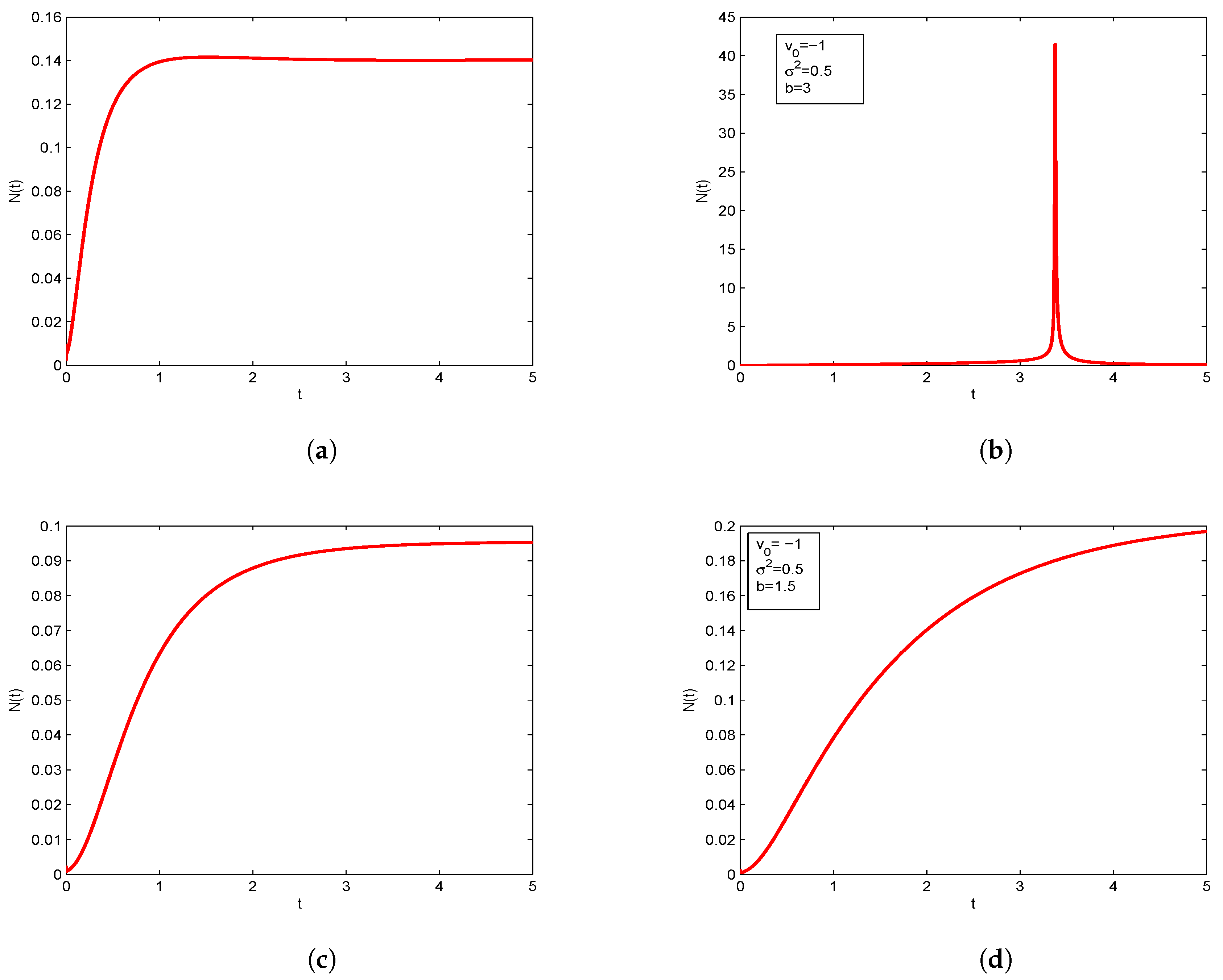
The evolution of firing rate
with the time
, is plotted in
Figure 2. We find that firing rate has different range with change in
excitatory case as well as the inhibitory case
In
Figure 2a, we consider the case when the initial data is centered at
with
We observe that the solution reaches a steady state. We also take the cases when the initial data is centered at
and different values of
to find different phenomena based on these values in
Figure 2.
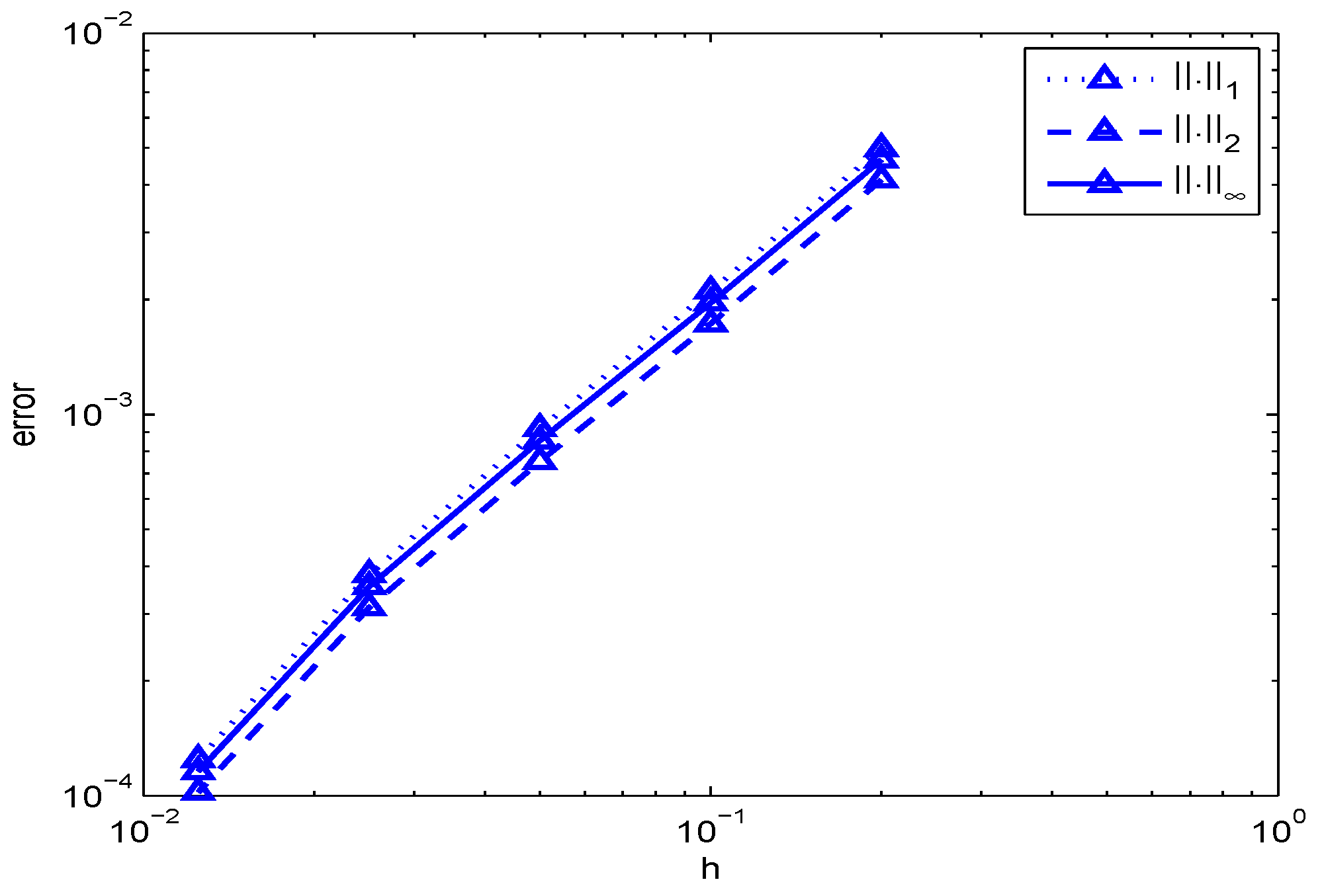
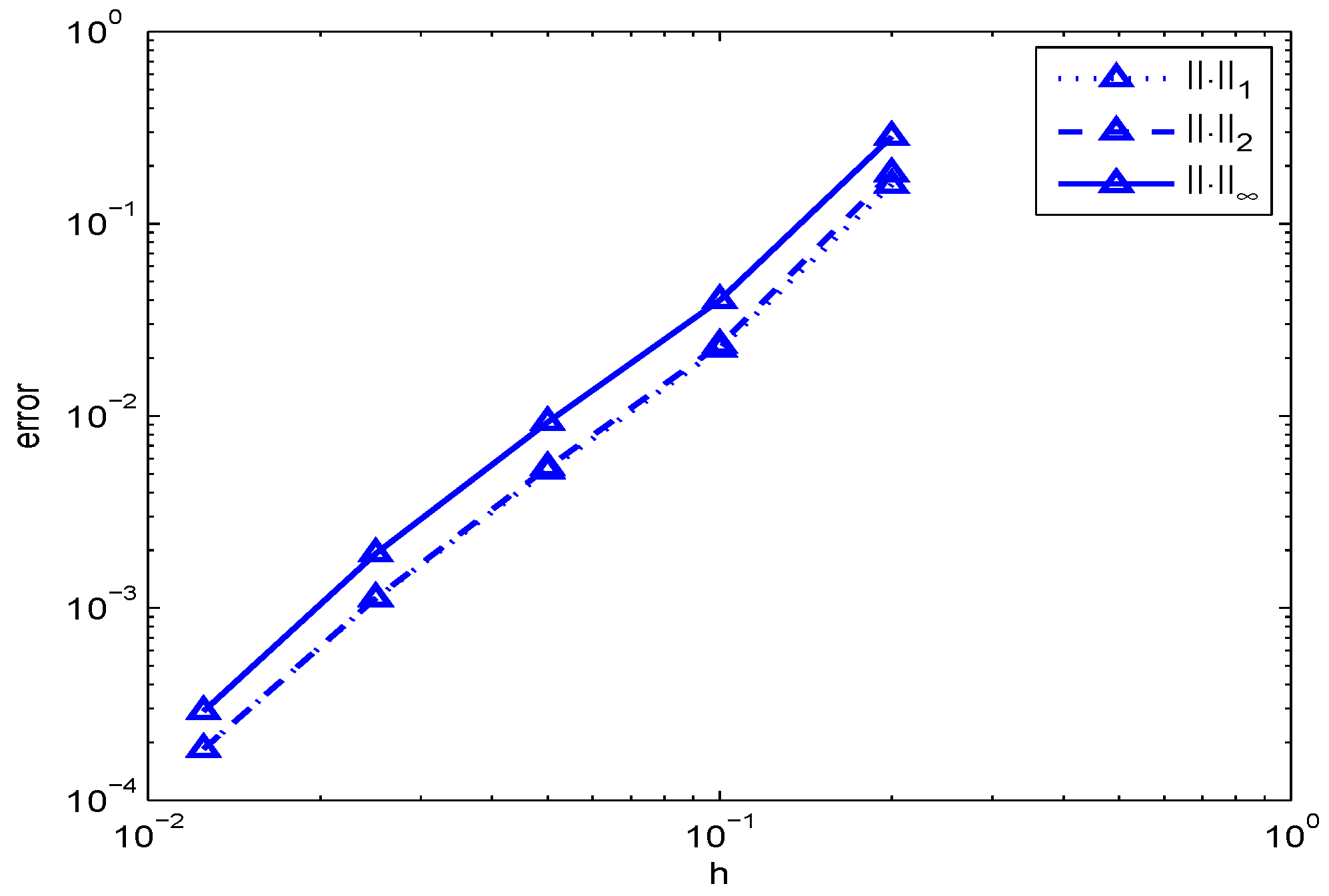
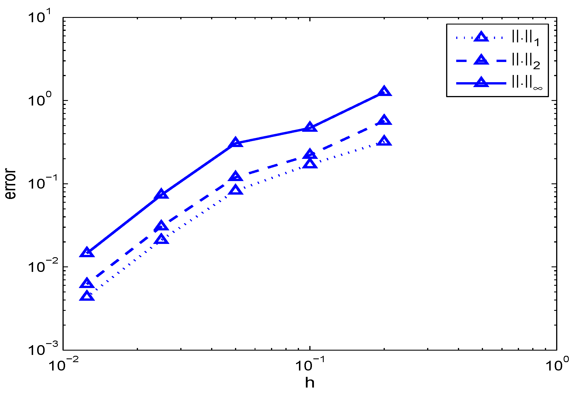
The errors for the approximate solution simulated in
Figure 1,
Figure 3 and
Figure 4 are plotted in
Figure 5,
Figure 6 and
Figure 7 respectively. Numerical values of these errors and CPU time (MATLAB and Statistics Toolbox Release 2013a, The MathWorks, Inc., Natick, MA, United States) of the two methods are shown in
Table 1 and
Table 2.
Errors of the numerical solution
are calculated in different norms
norms which are defined as follows
where
is the numerical solution at finest grid
For the numerical experiments, we find the errors with the finest grid being
Our test outcomes show that the error defined above is sure a monotone decreasing function as
N increases i.e.,
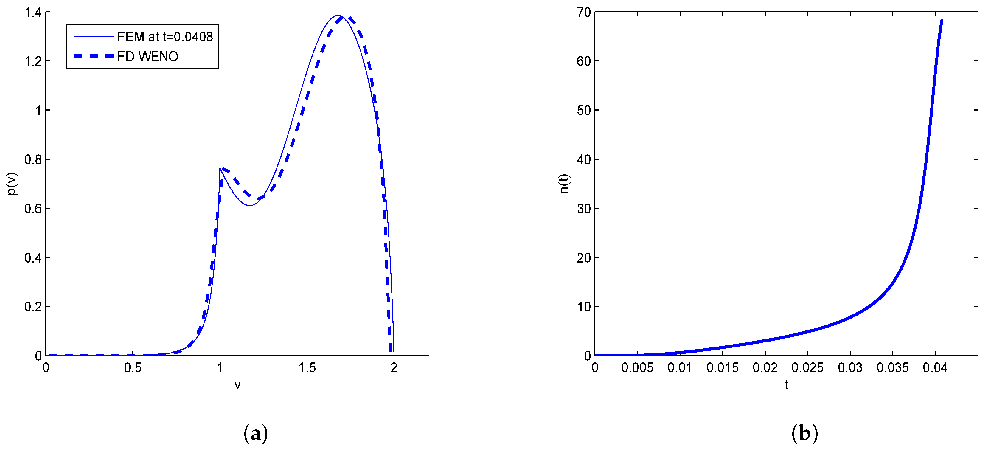
In
Figure 3a, we performed numerical approximation based upon FEM and compared the results obtained in [
8] at a time
The evolution of firing rate
with the time
, is plotted in
Figure 3b, which describes the blow-up situation when the initial data is concentrated around
with
Table 3 and
Table 4 gives the different error values at the final time
for the same data that is graphically represented in
Figure 6.
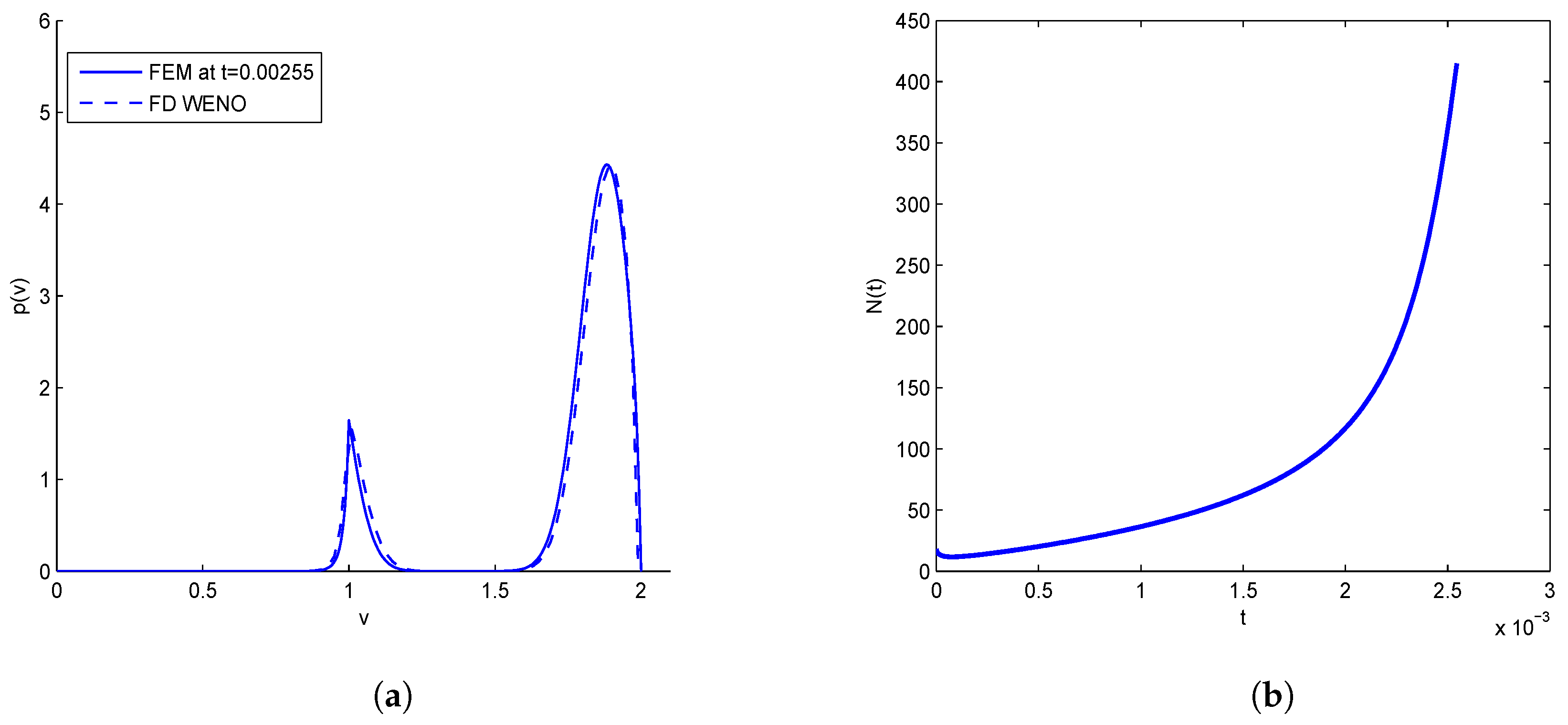
From
Figure 4a, it is clear that when initial data is concentrated enough near the threshold point
solution blows up at a finite time
which is earlier than the phenomena described in
Figure 3b. This happens because initial data is concentrated enough near the threshold point i.e.,
with
small enough. For different error values and CPU time for the data graphically represented in
Figure 4, see
Table 5 and
Table 6.
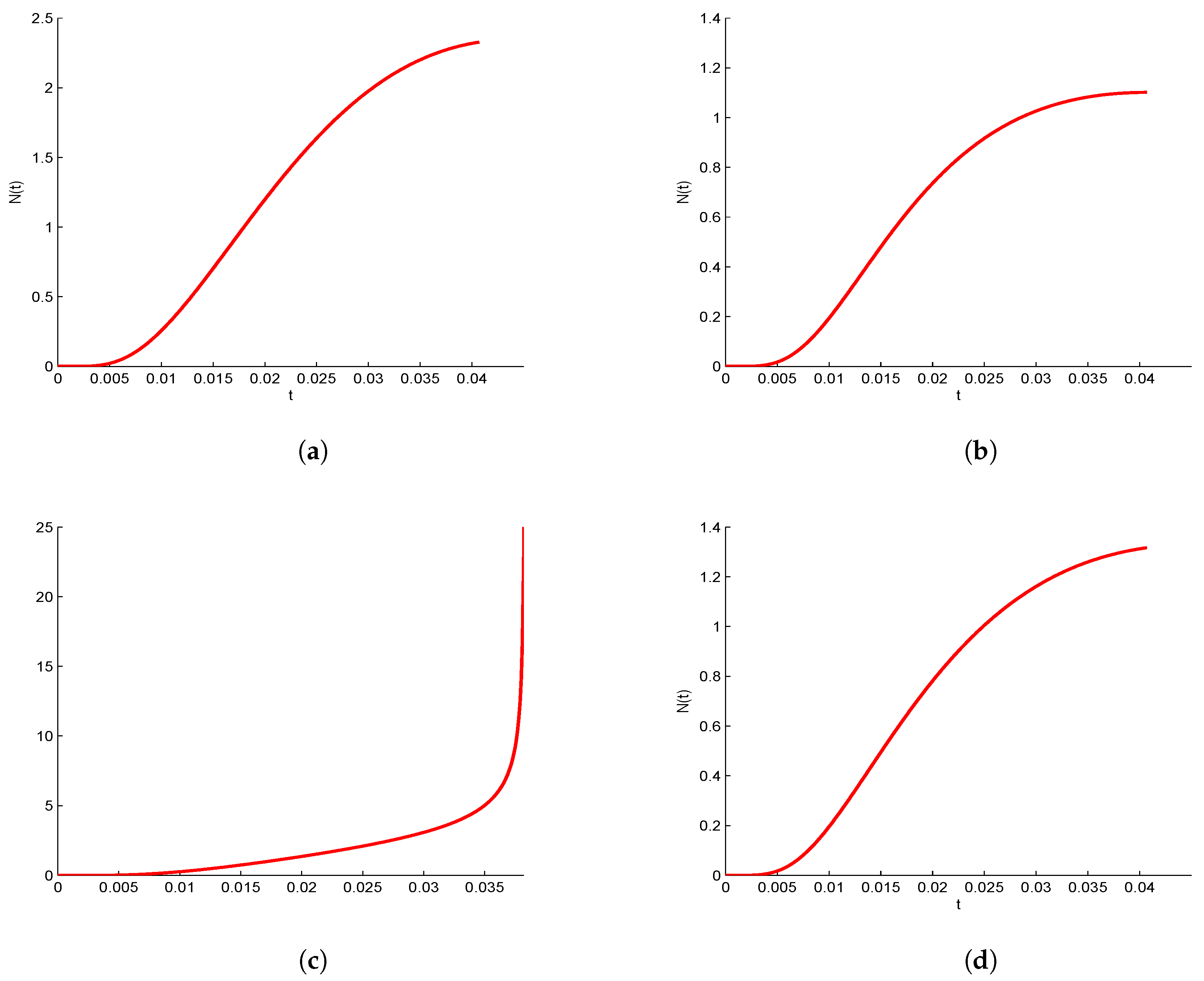
In
Figure 8, we treat the cases for
type activity dependence noise.
Figure 8a shows that by taking
and
solution goes to steady state. This further indicates that solution goes to a steady state earlier than the solution behavior provided in
Figure 8b by taking
.
Figure 8c shows blow-up situation of a solution by taking
and
. From
Figure 8d, we find that by reducing the noise factor
, solution goes to steady state.
The behavior of the solution by taking noise factor
for both the cases of excitatory and inhibitory are represented in
Figure 9. From
Figure 10a, we find that solution blows up in a finite time and right figure indicate the situation of steady state by reducing the noise factor.


