A Regularization Method to Solve a Cauchy Problem for the Two-Dimensional Modified Helmholtz Equation

Abstract

In this paper, the ill-posed problem of the two-dimensional modified Helmholtz equation is investigated in a strip domain. For obtaining a stable numerical approximation solution, a mollification regularization method with the de la Vallée Poussin kernel is proposed. An error estimate between the exact solution and approximation solution is given under suitable choices of the regularization parameter. Two numerical experiments show that our procedure is effective and stable with respect to perturbations in the data.

1. Introduction

The inversion problem on mathematical physics equations is an important branch in mathematics. The inversion of surface parameters in remote sensing science, the invention and application of CT in medical imaging, the reconstruction of optical signals and the geomorphological exploration in geological exploration are all related to such inversion problems [1].

There are many research methods and results for the Helmholtz equation for a positive wave number. The Helmholtz equation of a pure imaginary wave number is called the modified Helmholtz equation (also known as the Yukawa equation). It usually appears in the semi-implicit time-discrete heat equation and is also used to describe the physical phenomena of wave dispersion and diffusion [2]. A number of numerical solutions in the direct problem for the modified Helmholtz equation have been proposed [3,4], however, its inverse problem is severely ill-posed or improperly-posed in the viewpoint of Hadamard [5], the Cauchy problem suffers from the instability of the solution in the sense that a minor disturbance in the input data may cause a tremendous deviation in the solution [6]. To establish an accurate, stable, reliable and fast numerical algorithm for the Cauchy problem is a considerably interesting topic. It is impossible to solve this problem by using classical numerical methods, such as the finite element method (FEM), finite difference method (FDM) and finite volume method (FVM). It requires special techniques, and some different approaches had been given of an account of on the published literature, for instance, the Landweber method with boundary element method (BEM) [7], the conjugate gradient method [8], the method of fundamental solutions (MFS) [9], the Fourier regularization method [10], the truncation method [11] and the mollification method [12,13].

The kernel functions, such as Féjer kernel, Weierstrass kernel, Bessel-MacDonald kernel, de la Vallée Poussin kernel, Dirichlet and Krein kernel have a wide range of applications [12]. Manselli, Miller [13] and Murio [14] adopted the mollification method with the Weierstrass kernel to construct regularization operators to solve some inverse problems, but their methods were suitable for the case of Hilbert space $L^2\left(\mathbb{R}\right)$, furthermore they could not find appropriate regularization parameters. Hào [15] generalized their works, not only in Hilbert spaces, but also in Banach spaces with de la Vallée Poussin kernel and Dirichlet kernel. He applied the mollification method to concrete problems, such as the Cauchy problem of the Laplace equation, numerical differentiation and some parabolic equations. In recent years, inspired by Murio’s work [16], there are some research results for the mollification method with Gaussian kernel to solve Cauchy problem of elliptic equations [17,18,19].

In this paper, a mollification regular method with the de la Vallée Poussin kernel is introduced to solve the Cauchy problem for a Helmholtz-type equation; our approximation is to transform the ill-posed problem into a well-posed problem by convoluting the de la Vallée Poussin function and the measured data. We consider the following two problems:

$$\begin{array}{c}\left\{\begin{array}{c}∆u(x,y)-k^{2}u(x,y)=0,0<x<d,y\in \mathbb{R},\\ u(0,y)=f\left(y\right),y\in \mathbb{R},\\ u_x(0,y)=0,y\in \mathbb{R},\\ u(d,y)=h_1\left(y\right),y\in \mathbb{R},\end{array}\right.\end{array}$$

(1)

and

$$\begin{array}{c}\left\{\begin{array}{c}∆v(x,y)-k^{2}v(x,y)=0,0<x<d,y\in \mathbb{R},\\ v(0,y)=0,y\in \mathbb{R},\\ v_x(0,y)=g\left(y\right),y\in \mathbb{R},\\ v(d,y)=h_2\left(y\right),y\in \mathbb{R},\end{array}\right.\end{array}$$

(2)

where $∆=\frac{{\partial }^2}{\partial x^2}+\frac{{\partial }^2}{\partial y^2}$ is a two-dimensional Laplace operator, $f\left(y\right)$, $g\left(y\right)$ are given vectors in $L^2\left(\mathbb{R}\right)$, and $h_1\left(y\right),h_1\left(y\right)\in L^2\left(\mathbb{R}\right)$ are unknown vectors. The constant k $(k>0)$ is the wave number.

Let $w=u+v$, where u and v are solution of problems (1) and (2), respectively. Then w is the solution of the following Cauchy problem with the inhomogeneous Neumann boundary condition:

$$\begin{array}{c}\left\{\begin{array}{c}∆w(x,y)-k^{2}w(x,y)=0,0<x<d,y\in \mathbb{R},\\ w(0,y)=f\left(y\right),y\in \mathbb{R},\\ w_x(0,y)=g\left(y\right),y\in \mathbb{R},\\ w(d,y)=h\left(y\right),y\in \mathbb{R},\end{array}\right.\end{array}$$

(3)

where $h\left(y\right)=h_1\left(y\right)+h_2\left(y\right)$.

We assume that all the functions involved are $L^2$ functions in $(-\infty ,\infty )$, Additionally suppose that input functions $f\left(y\right)$, $g\left(y\right)$ and its measurement data $f^{\delta }\left(y\right)$, $g^{\delta }\left(y\right)$ satisfy

$$max\{\parallel f-f^{\delta }\parallel ,\parallel g-g^{\delta }\parallel \parallel \}\le \delta ,$$

(4)

where $\delta >0$ denotes noise level, and $\parallel ·\parallel$ denotes the $L^2—$norm.

Assume there exits a constant $E>0$, such that the following a priori bound holds:

$$max\{\parallel h_1(·)\parallel ,\parallel h_2(·)\parallel \}\le E.$$

(5)

The rest of this paper is organized as follows. In Section 2, we illuminate the ill-posed nature of problems (1) and (2), the de la Vallée Poussin kernel and some properties are presented to obtain the regularization solution. In Section 3, some error estimates are given for $0<x<d$ and at the boundary $x=d$ under the suitable choices of regularization parameter. Section 4 is the numerical aspect of our proposed algorithm. Some conclusions are given in Section 5.

2. Description of the Problem and Mollification Method

Let us introduce the Sobolev space $H^r\left(\mathbb{R}\right)$ [15] with $r\ge 0$, and if $r=0$, then $H^0=L^2\left(\mathbb{R}\right)$, $H^r=\{f\left(y\right)\in L^2{\left(\mathbb{R}\right):\parallel f\parallel }_{H^r}<\infty \}$, where

$${\parallel f\parallel }_{H^r}:=({\int }_{\mathbb{R}}|\widehat{f}\left(\xi \right){{|}^2{(1+{\xi }^2)}^{r}d\xi )}^{1/2}$$

(6)

with the Fourier transform

$$\begin{array}{c}\widehat{f}\left(\xi \right)=\frac{1}{\sqrt{2\pi }}{\int }_{\mathbb{R}}{e}^{-i\xi ·y}dy,(\xi \in \mathbb{R})\end{array}$$

Additionally, the inverse Fourier transform for the variable $\xi \in \mathbb{R}$

$$f\left(y\right)=\frac{1}{\sqrt{2\pi }}{\int }_{\mathbb{R}}{e}^{i\xi ·y}\widehat{f}\left(\xi \right)d\xi .$$

In this paper, we denote $\parallel ·\parallel :={\parallel ·\parallel }_0$.

For any function $\phi \in L^1\left(\mathbb{R}\right)$ and $f\in L^p\left(\mathbb{R}\right)$, $1\le p\le \infty$, the convolution is defined by [15]

$$\phi \ast f=\frac{1}{\sqrt{2\pi }}{\int }_{-\infty }^{+\infty }\phi (x-y)f\left(y\right)dy=\frac{1}{\sqrt{2\pi }}{\int }_{-\infty }^{+\infty }\phi \left(y\right)f(x-y)dy.$$

(7)

It is well known that [16]

$$\widehat{(\phi \ast f)}\left(\xi \right)=\widehat{\phi }\left(\xi \right)\widehat{f}\left(\xi \right),$$

(8)

and

$${\parallel \phi \ast f\parallel }_p\le \frac{1}{\sqrt{2\pi }}{\parallel \phi \parallel }_1{\parallel f\parallel }_p,$$

(9)

and the Parseval equality [15]

$$\parallel f\parallel =\parallel \widehat{f}\parallel ,f,\widehat{f}\in L^2\left(\mathbb{R}\right).$$

(10)

2.1. Ill-posed Analysis

Applying the Fourier transform to problems (1) and (2). with respect to the variable y, we obtain the following problems:

$$\begin{array}{c}\left\{\begin{array}{c}{\widehat{u}}_{xx}(x,\xi )+{\left(i\xi \right)}^2\widehat{u}(x,\xi )-k^2\widehat{u}(x,\xi )=0,0<x<d,\xi \in \mathbb{R};\\ \widehat{u}(0,\xi )=\widehat{f}\left(\xi \right),\xi \in \mathbb{R};\\ {\widehat{u}}_x(0,\xi )=0,\xi \in \mathbb{R}.\end{array}\right.\end{array}$$

(11)

and

$$\begin{array}{c}\left\{\begin{array}{c}{\widehat{v}}_{xx}(x,\xi )+{\left(i\xi \right)}^2\widehat{v}(x,\xi )-k^2\widehat{v}(x,\xi )=0,0<x<d,\xi \in \mathbb{R};\\ \widehat{v}(0,\xi )=0,\xi \in \mathbb{R};\\ {\widehat{v}}_x(0,\xi )=\widehat{g}\left(\xi \right),\xi \in \mathbb{R}.\end{array}\right.\end{array}$$

(12)

The solution of problem (11) is

$$\widehat{u}(x,\xi )=\widehat{f}\left(\xi \right)cosh\left(x\sqrt{{\xi }^2+k^2}\right).$$

or equivalently,

$$u(x,y)=\frac{1}{\sqrt{2\pi }}{\int }_{-\infty }^{+\infty }\widehat{f}\left(\xi \right)cosh\left(x\sqrt{{\xi }^2+k^2}\right)e^{i\xi y}d\xi .$$

The solution of problem (12) is

$$\widehat{v}(x,\xi )=\widehat{g}\left(\xi \right)\frac{sinh\left(x\sqrt{{\xi }^2+k^2}\right)}{\sqrt{{\xi }^2+k^2}}.$$

or equivalently,

$$v(x,y)=\frac{1}{\sqrt{2\pi }}{\int }_{-\infty }^{+\infty }\widehat{g}\left(\xi \right)\frac{sinh\left(x\sqrt{{\xi }^2+k^2}\right)}{\sqrt{{\xi }^2+k^2}}{e}^{i\xi y}d\xi .$$

When $x=d$, we have

$$\widehat{u}(d,\xi )=\widehat{f}\left(\xi \right)cosh\left(d\sqrt{{\xi }^2+k^2}\right),\widehat{v}(d,\xi )=\widehat{g}\left(\xi \right)\frac{sinh\left(d\sqrt{{\xi }^2+k^2}\right)}{\sqrt{{\xi }^2+k^2}}.$$

Apparently, the factors $cosh\left(x\sqrt{{\xi }^2+k^2}\right)$ and $\frac{sinh\left(x\sqrt{{\xi }^2+k^2}\right)}{\sqrt{{\xi }^2+k^2}}$ are unbounded with respect to variable $\xi$, a small perturbation in the measured data $\widehat{g}\left(\xi \right)$ and $\widehat{h}\left(\xi \right)$ may arouse a tremendously large error in the solutions $u(x,y)$ and $v(x,y)$, respectively. Therefore, problems (1), (2) and (3) are severely ill-posed [5].

2.2. Mollification Method

This paper is devoted to establishing a mollification method, constructing mollification operator by convolution with the de la Vallée Poussin kernel and measurement data, as thus the ill-posed problems are transformed into well-posed problems.

The function

$$V_{\alpha }\left(t\right)=\frac{cos\left(\alpha t\right)-cos\left(2\alpha t\right)}{\alpha t^2}.$$

is called the de la Vallée Poussin kernel [15]. Here, $\alpha$ $(\alpha >0)$ is called mollification radius or mollification parameter, and $V_{\alpha }\left(x\right)$ has the following properties [15].

(1) $V_{\alpha }\left(t\right)$ is an exponential type entire function of degree $2\alpha$ relative variable t, bounded and summable on $\mathbb{R}$;

(2) ${\widehat{V}}_{\alpha }$ is the Fourier transform of $V_{\alpha }\left(t\right)$ and satisfies

$$\begin{array}{c}\sqrt{\frac{2}{\pi }}{\widehat{V}}_{\alpha }=\left\{\begin{array}{c}1,\left|\xi \right|<\alpha ,\\ \frac{2\alpha -\xi }{\alpha },\alpha <\left|\xi \right|\le 2\alpha ,\\ 0,\left|\xi \right|>2\alpha ;\end{array}\right.\end{array}$$

(3) $\frac{1}{\pi }{\int }_{-\infty }^{+\infty }{V}_{\alpha }\left(t\right)dt=1$;

(4) $\frac{1}{\pi }{\int }_{-\infty }^{+\infty }\left|V_{\alpha }\left(t\right)\right|dt<2\sqrt{3}(\alpha \ge 1)$.

We define the operator $T_{\alpha }$ by $T_{\alpha }:\mathbb{R}\to \mathbb{R}$

$$\left(T_{\alpha }{f}^{\delta }\right)\left(t\right)=\frac{1}{\pi }{\int }_{-\infty }^{+\infty }{V}_{\alpha }(t-y)f^{\delta }\left(y\right)dy=\sqrt{\frac{2}{\pi }}(V_{\alpha }\ast f^{\delta })\left(t\right),$$

Utilizing (8), we have

$$\widehat{\left(T_{\alpha }{f}^{\delta }\right)}\left(\xi \right)=\sqrt{2/\pi }{\widehat{V}}_{\alpha }\left(\xi \right){\widehat{f}}^{\delta }\left(\xi \right),$$

The Cauchy problems (1) and (2) can be stabilized, if instead of attempting to find the values of the function $f^{\delta }\left(y\right)$, $g^{\delta }\left(y\right)$, we shall reconstruct the $\delta —$mollification of the function $f^{\delta }\left(y\right)$, $g^{\delta }\left(y\right)$, given by $\left(T_{\alpha }{f}^{\delta }\right)\left(y\right)$, $\left(T_{\alpha }{g}^{\delta }\right)\left(y\right)$. We have the following problems with the mollified data:

$$\begin{array}{c}\left\{\begin{array}{c}{u}_{xx}^{\alpha ,\delta }+u_{yy}^{\alpha ,\delta }-k^2{u}^{\alpha ,\delta }=0,0<x<d,y\in \mathbb{R},\\ u^{\alpha ,\delta }(0,y)=\left(T_{\alpha }{f}^{\delta }\right)\left(y\right),y\in \mathbb{R},\\ u_x^{\alpha ,\delta }(0,y)=0,y\in \mathbb{R},\end{array}\right.\end{array}$$

(13)

and

$$\begin{array}{c}\left\{\begin{array}{c}{v}_{xx}^{\alpha ,\delta }+v_{yy}^{\alpha ,\delta }-k^2{v}^{\alpha ,\delta }=0,0<x<d,y\in \mathbb{R},\\ v^{\alpha ,\delta }(0,y)=0,y\in \mathbb{R},\\ v_x^{\alpha ,\delta }(0,y)=\left(T_{\alpha }{g}^{\delta }\right)\left(y\right),y\in \mathbb{R},\end{array}\right.\end{array}$$

(14)

where $u^{\alpha ,\delta }$ and $v^{\alpha ,\delta }$ denote the solution of problems (13) and (14), respectively.

The solution of problem (13) is

$${\widehat{u}}^{\alpha ,\delta }(x,\xi )=\widehat{\left(T_{\alpha }{f}^{\delta }\right)}\left(\xi \right)cosh\left(x\sqrt{{\xi }^2+k^2}\right),$$

equivalently

$$u^{\alpha ,\delta }(x,y)=\frac{1}{\sqrt{2\pi }}{\int }_{-\infty }^{+\infty }\widehat{\left(T_{\alpha }{f}^{\delta }\right)}\left(\xi \right)cosh\left(x\sqrt{{\xi }^2+k^2}\right)e^{i\xi y}d\xi .$$

The solution of problem (14) is

$${\widehat{v}}^{\alpha ,\delta }(x,\xi )=\widehat{\left(T_{\alpha }{g}^{\delta }\right)}\left(\xi \right)\frac{sinh\left(x\sqrt{{\xi }^2+k^2}\right)}{\sqrt{{\xi }^2+k^2}},$$

equivalently

$$v^{\alpha ,\delta }(x,y)=\frac{1}{\sqrt{2\pi }}{\int }_{-\infty }^{+\infty }\widehat{\left(T_{\alpha }{g}^{\delta }\right)}\left(\xi \right)\frac{sinh\left(x\sqrt{{\xi }^2+k^2}\right)}{\sqrt{{\xi }^2+k^2}}{e}^{i\xi y}d\xi .$$

According to the property (3) of kernel function $V_{\alpha }$, we have

$$T_{\alpha }{f}^{\delta }\left(y\right)-f\left(y\right)=\frac{1}{\pi }{\int }_{-\infty }^{+\infty }{V}_{\alpha }\left(s\right)(f^{\delta }(y-s)-f\left(y\right))ds.$$

From (9) and property (4) of $V_{\alpha }$, we get

$$\parallel T_{\alpha }{f}^{\delta }{-f\parallel }_2\le \parallel V_{\alpha }{\parallel }_1·{\parallel f-f^{\delta }\parallel }_2<2\sqrt{3}\delta .$$

Remark 1.

Assumption that condition (4) is valid, when $\alpha \ge 1$, we have

$$\parallel T_{\alpha }{f}^{\delta }{-f\parallel }_2<2\sqrt{3}\delta ,{\parallel T_{\alpha }{f}^{\delta }-f\parallel }_2<2\sqrt{3}\delta .$$

3. Error Estimate and Parameter Selection

Lemma 1.

For $0<x\le d$, the following inequalities hold.

(1) $\frac{sinh\left(x\sqrt{{\xi }^2+k^2}\right)}{sinh\left(d\sqrt{{\xi }^2+k^2}\right)}\le e^{-(d-x)\left|\xi \right|}$;

(2) $\frac{sinh\left(x\sqrt{{\xi }^2+k^2}\right)}{\sqrt{{\xi }^2+k^2}}\le d{e}^{x\left(\right|\xi |+k)}$;

(3) $\frac{cosh\left(x\sqrt{{\xi }^2+k^2}\right)}{cosh\left(d\sqrt{{\xi }^2+k^2}\right)}\le 2e^{-(d-x)\left|\xi \right|}$;

(4) $cosh\left(x\sqrt{{\xi }^2+k^2}\right)\le e^{x\left(\right|\xi |+k)}$.

Proof. 

Using inequality $\left|\xi \right|<\sqrt{{\xi }^2+k^2}<\left|\xi \right|+k$, the proofs of (3) and (4) can be obtained. Therefore, we only prove (1) and (2).

From inequality,

$$\begin{array}{c}\frac{sinh\left(x\sqrt{{\xi }^2+k^2}\right)}{sinh\left(d\sqrt{{\xi }^2+k^2}\right)}=\frac{e^{x\sqrt{{\xi }^2+k^2}}}{e^{d\sqrt{{\xi }^2+k^2}}}·\frac{1-e^{-2x\sqrt{{\xi }^2-k^2}}}{1-e^{-2d\sqrt{{\xi }^2-k^2}}}\le \frac{e^{x\sqrt{{\xi }^2+k^2}}}{e^{d\sqrt{{\xi }^2+k^2}}},\end{array}$$

inequality (1) can be arrived at.

By the Taylor’s expansion,

$$\begin{array}{cc}\frac{sinh\left(x\sqrt{{\xi }^2+k^2}\right)}{\sqrt{{\xi }^2+k^2}}& =\frac{1}{\sqrt{{\xi }^2+k^2}}\sum _{n=0}^{\infty }\frac{{\left(x\sqrt{{\xi }^2+k^2}\right)}^{2n+1}}{(2n+1)!}=\sum _{n=0}^{\infty }\frac{{\left(\sqrt{{\xi }^2+k^2}\right)}^{2n}{x}^{2n+1}}{(2n+1)!}\hfill \\ & \le d\sum _{n=0}^{\infty }\frac{{\left(x\sqrt{{\xi }^2+k^2}\right)}^{2n}}{\left(2n\right)!}=dcosh\left(x\sqrt{{\xi }^2+k^2}\right),\hfill \end{array}$$

we obtain (2). □

In the following, we will give error estimate for $\parallel u-u^{\alpha ,\delta }\parallel$, $\parallel v-v^{\alpha ,\delta }\parallel$ and $\parallel w-w^{\alpha ,\delta }\parallel$ in $0<x<d$ and at boundary $x=d$, respectively. The convergence results will be obtained while we choose a suitable regular parameter $\alpha$.

3.1. Approximation Theorems

In this section, we shall give the stable estimates of the proposed regularization method for the case of $0<x<d$.

Theorem 1.

Let $u(x,y)$ be the exact solution of problem (1) with the exact input data $f\left(y\right)$, and let $u^{\alpha ,\delta }(x,y)$ be the regularized solution of problem (13) with the noisy data $f^{\delta }\left(y\right)$. Assume that conditions (4) and (5) hold, we have the following estimate:

$$\parallel u-u^{\alpha ,\delta }\parallel <12E{e}^{-(d-x)\alpha }+7\delta e^{x(2\alpha +k)}.$$

(15)

Furthermore, if we select regular parameter α as

$$\alpha =\frac{1}{2d}ln(E/\delta ),$$

(16)

we obtain

$$\parallel u-u^{\alpha ,\delta }\parallel <12E^{(d+x)/2d}{\delta }^{(d-x)/2d}+7e^{xk}{E}^{x/d}{\delta }^{1-x/d}.$$

(17)

Proof. 

Suppose that conditions (4) and (5) hold, using Parseval formula (10), we have

$$\begin{array}{c}\parallel u-u^{\alpha ,\delta }{\parallel }^2={\parallel \widehat{u}-{\widehat{u}}^{\alpha ,\delta }\parallel }^2\hfill \\ ={\int }_{-\infty }^{-2\alpha }|P\left(\xi \right)\widehat{f}{\left(\xi \right)|}^{2}d\xi +{\int }_{-2\alpha }^{-\alpha }{\left|P\left(\xi \right)(\widehat{f}\left(\xi \right)-\frac{2\alpha -\xi }{\alpha }{\widehat{f}}^{\delta }\left(\xi \right))\right|}^{2}d\xi +\hfill \\ {\int }_{-\alpha }^{\alpha }\left|P\left(\xi \right)\right(\widehat{f}\left(\xi \right)-{\widehat{f}}^{\delta }{\left(\xi \right)|}^{2}d\xi +{\int }_{\alpha }^{2\alpha }{\left|P\left(\xi \right)(\widehat{f}\left(\xi \right)-\frac{2\alpha -\xi }{\alpha }{\widehat{f}}^{\delta }\left(\xi \right))\right|}^{2}d\xi \hfill \\ +{\int }_{2\alpha }^{+\infty }{\left|P\left(\xi \right)\widehat{f}\left(\xi \right)\right|}^{2}d\xi ,\hfill \end{array}$$

where

$$P\left(\xi \right)=cosh\left(x\sqrt{{\xi }^2+k^2}\right),(\xi \in \mathbb{R}).$$

If $\xi \in [\alpha ,2\alpha ]$, then $0<\frac{\xi -\alpha }{\alpha }<1$.

According to Minkowski inequality, there is

$$\begin{array}{c}({\int }_{\alpha }^{2\alpha }|P\left(\xi \right)(\widehat{f}\left(\xi \right)-\frac{2\alpha -\xi }{\alpha }{\widehat{f}}^{\delta }\left(\xi \right)){{|}^{2}d\xi )}^{1/2}\hfill \\ =\left|\right|P\left(\xi \right)(\widehat{f}\left(\xi \right)-{\widehat{f}}^{\delta }\left(\xi \right)+\frac{\xi -\alpha }{\alpha }{\widehat{f}}^{\delta }\left(\xi \right)){\left|\right|}_{H^0[\alpha ,2\alpha ]}\hfill \\ \le \parallel P\left(\xi \right)(\widehat{f}\left(\xi \right)-{\widehat{f}}^{\delta }\left(\xi \right){\parallel }_{H^0[\alpha ,2\alpha ]}+\parallel P\left(\xi \right){\widehat{f}}^{\delta }\left(\xi \right){\parallel }_{H^0[\alpha ,2\alpha ]}\hfill \\ \le 2\parallel P\left(\xi \right)(\widehat{f}\left(\xi \right)-{\widehat{f}}^{\delta }\left(\xi \right){\parallel }_{H^0[\alpha ,2\alpha ]}+\parallel P\left(\xi \right)\widehat{f}\left(\xi \right){\parallel }_{H^0[\alpha ,2\alpha ]}\hfill \\ \le 2\parallel P\left(\xi \right)(\widehat{f}\left(\xi \right)-{\widehat{f}}^{\delta }\left(\xi \right)\parallel +\parallel A\left(\xi \right)\widehat{h_1}\left(\xi \right)\parallel \hfill \\ \le 2\delta \underset{\left|\xi \right|\in [\alpha ,2\alpha ]}{sup}\left|P\left(\xi \right)\right|+E\underset{\left|\xi \right|\in [\alpha ,2\alpha ]}{sup}\left|A\left(\xi \right)\right|,\hfill \end{array}$$

where,

$$A\left(\xi \right)=\frac{cosh\left(x\sqrt{{\xi }^2+k^2}\right)}{cosh\left(d\sqrt{{\xi }^2+k^2}\right)},(\xi \in \mathbb{R}).$$

Therefore, we have

$$\begin{array}{c}\parallel u-u^{\alpha ,\delta }{\parallel }^2={\parallel \widehat{u}-{\widehat{u}}^{\alpha ,\delta }\parallel }^2\hfill \\ \le 2E^2(\underset{\left|\xi \right|\ge 2\alpha }{sup}{\left|A\left(\xi \right)\right|)}^2+(4\delta \underset{\xi \in [-2\alpha ,-\alpha ]}{sup}\left|P\left(\xi \right)\right|+3E\underset{\xi \in [-2\alpha ,-\alpha ]}{sup}{\left|A\left(\xi \right)\right|)}^2+\hfill \\ {\delta }^2(\underset{\xi \in [-\alpha ,\alpha ]}{sup}{\left|P\left(\xi \right)\right|)}^2+(2\delta \underset{\xi \in [\alpha ,2\alpha ]}{sup}\left|P\left(\xi \right)\right|+E\underset{\xi \in [\alpha ,2\alpha ]}{sup}{\left|A\left(\xi \right)\right|)}^2.\hfill \end{array}$$

From items (3) and (4) of Lemma 1, we have

$$\begin{array}{c}\parallel u-u^{\alpha ,\delta }{\parallel }^2\hfill \\ \le 8E^2{e}^{-(d-x)4\alpha }+{(4\delta e^{x(2\alpha +k)}+6E{e}^{-(d-x)\alpha })}^2+\hfill \\ {\delta }^2{e}^{2x(\alpha +k)}+{(2\delta e^{x(2\alpha +k)}+2E{e}^{-(d-x)\alpha })}^2.\hfill \end{array}$$

Using inequality $\sqrt{A+B}<\sqrt{A}+\sqrt{B}$ $(A>0,B>0)$, we obtain

$$\begin{array}{c}\parallel u-u^{\alpha ,\delta }\parallel \hfill \\ <4E{e}^{-(d-x)2\alpha }+4\delta e^{x(2\alpha +k)}+6E{e}^{-(d-x)\alpha }+\delta e^{x(\alpha +k)}+2\delta e^{x(2\alpha +k)}+2E{e}^{-(d-x)\alpha }\hfill \\ <12E{e}^{-(d-x)\alpha }+7\delta e^{x(2\alpha +k)}.\hfill \end{array}$$

Choosing the parameter $\alpha$ as (16), then (17) holds. □

Similarly, we have the following error estimate for problem (2).

Theorem 2.

Let $v(x,y)$ be the exact solution of problem (2) with the exact input data $g\left(y\right)$, and let $v^{\alpha ,\delta }(x,y)$ be the regularized solution of problem (14) with the noisy data $g^{\delta }\left(y\right)$. Assume that conditions (4) and (5) hold, we have the following estimate:

$$\parallel v-v^{\alpha ,\delta }\parallel <6E{e}^{-(d-x)\alpha }+7d\delta e^{x(2\alpha +k)}.$$

(18)

Furthermore, if we select regular parameter α as (16), then

$$\parallel v-v^{\alpha ,\delta }\parallel <6E^{(d+x)/2d}{\delta }^{(d-x)/2d}+7d{e}^{xk}{E}^{x/d}{\delta }^{1-x/d}.$$

(19)

Moreover, according to the results of Theorems 1 and 2 and Minkowski inequality, we get the Theorem 3 as follows.

Theorem 3.

Let $w(x,y)$ be the exact solution of problem (3) with the exact input data $f\left(y\right)$, $g\left(y\right)$, and let $w^{\alpha ,\delta }(x,y)$ be its approximate solution with the noisy data $f^{\delta }\left(y\right)$, $g^{\delta }\left(y\right)$. Assume that conditions (4) and (5) hold, we have the following estimate:

$$\parallel w-w^{\alpha ,\delta }\parallel <18E{e}^{-(d-x)\alpha }+7(d+1)\delta e^{x(2\alpha +k)}.$$

(20)

Furthermore, if we select regular parameter α as (16), then

$$\parallel w-w^{\alpha ,\delta }\parallel <18E^{(d+x)/2d}{\delta }^{(d-x)/2d}+7(d+1)e^{xk}{E}^{x/d}{\delta }^{1-x/d}.$$

(21)

3.2. Approximation Estimate at Boundary

Note that the error estimates in above section only solve our problems for $0<x<d$ and do not give any useful information at $x=d$. In order to obtain the stability estimates of problems (1) and (2) at $x=d$, we need a stronger a priori assumption instead of (5):

$$max\{\parallel h_1{(·)\parallel }_{H^r},\parallel h_2(·){\parallel }_{H^r}\}\le E_r,r>0,$$

(22)

where constant $E_r>0$ dependents only on r.

Theorem 4.

Let $u(d,y)$ be the solution of the Cauchy problem (1) and $u^{\alpha ,\delta }(d,y)$ be solution of modified problem (13) at $x=d$. Suppose that conditions (4) and (22) hold, we have

$$\parallel u(d,·)-u^{\alpha ,\delta }(d,·)\parallel <\frac{6E_r}{{(1+{\alpha }^2)}^{r/2}}+7\delta e^{d(2\alpha +k)}.$$

(23)

If we select

$$\alpha =\frac{1}{4d}ln(E_r/\delta ),$$

(24)

there is

$$\parallel u(d,·)-u^{\alpha ,\delta }(d,·)\parallel <6E_r{(\frac{4d}{ln(E_r/\delta )})}^r+7E_r^{1/2}{e}^{dk}{\delta }^{1/2}.$$

(25)

Proof. 

From equality (10), adoption similar analysis method with Theorem 1, we have

$$\begin{array}{c}\parallel u(d,·)-u^{\alpha ,\delta }{(d,·)\parallel }^2={\parallel \widehat{u}(d,·)-{\widehat{u}}^{\alpha ,\delta }(d,·)\parallel }^2\hfill \\ ={\int }_{-\infty }^{-2\alpha }|\frac{1}{{(1+{\xi }^2)}^{r/2}}{(1+{\xi }^2)}^{r/2}\widehat{u}(d,\xi ){|}^{2}d\xi +{\int }_{-2\alpha }^{-\alpha }{|P\left(\xi \right)(\widehat{f}\left(\xi \right)-\frac{2\alpha -\xi }{\alpha }{\widehat{f}}_{\delta }\left(\xi \right))|}^{2}d\xi +\hfill \\ {\int }_{-\alpha }^{\alpha }\left|P\left(\xi \right)\right(\widehat{f}\left(\xi \right)-{\widehat{f}}^{\delta }{\left(\xi \right)|}^{2}d\xi +{\int }_{\alpha }^{2\alpha }{|P\left(\xi \right)(\widehat{f}\left(\xi \right)-\frac{2\alpha -\xi }{\alpha }{\widehat{f}}^{\delta }\left(\xi \right))|}^{2}d\xi +\hfill \\ {\int }_{2\alpha }^{+\infty }{|\frac{1}{{(1+{\xi }^2)}^{r/2}}{(1+{\xi }^2)}^{r/2}\widehat{u}(d,\xi )|}^{2}d\xi \hfill \\ \le 2E_r^2(\underset{\left|\xi \right|\ge 2\alpha }{sup}{\left|B\left(\xi \right)\right|)}^2+(4\delta \underset{\xi \in [-2\alpha ,-\alpha ]}{sup}\left|P\left(\xi \right)\right|+3E_r\underset{\xi \in [-2\alpha ,-\alpha ]}{sup}{\left|B\left(\xi \right)\right|)}^2+\hfill \\ {\delta }^2(\underset{\xi \in [-\alpha ,\alpha ]}{sup}{\left|P\left(\xi \right)\right|)}^2+(2\delta \underset{\xi \in [\alpha ,2\alpha ]}{sup}\left|P\left(\xi \right)\right|+E_r\underset{\xi \in [\alpha ,2\alpha ]}{sup}{\left|B\left(\xi \right)\right|)}^2,\hfill \end{array}$$

where

$$B\left(\xi \right)=\frac{1}{{(1+{\xi }^2)}^{r/2}},P\left(\xi \right)=cosh\left(d\sqrt{{\xi }^2+k^2}\right),(\xi \in \mathbb{R}).$$

Applying (4) of Lemma 1, we have

$$\begin{array}{c}\parallel u(d,·)-u^{\alpha ,\delta }(d,·)\parallel <\frac{6E_r}{{(1+{\alpha }^2)}^{r/2}}+7\delta e^{d(2\alpha +k)}.\end{array}$$

Taking regularization parameter $\alpha$ as (24), then (25) holds. □

Similarly, combining (2) of Lemma 1, we have error estimation of problem (2) at boundary $x=d$.

Theorem 5.

Let $v(d,y)$ be the solution of the Cauchy problem (2) and $v^{\alpha ,\delta }(d,y)$ be the solution of modified problem (14) at $x=d$. Suppose that conditions (4) and (22) hold, we have

$$\parallel v(d,·)-v^{\alpha ,\delta }(d,·)\parallel <\frac{6E_r}{{(1+{\alpha }^2)}^{r/2}}+7d\delta e^{d(2\alpha +k)}.$$

(26)

If we select α as (24), then

$$\parallel v(d,·)-v^{\alpha ,\delta }(d,·)\parallel <6E_r{(\frac{4d}{ln(E_r/\delta )})}^r+7d{E}_r^{1/2}{e}^{dk}{\delta }^{1/2}.$$

(27)

According the results of Theorem 4, Theorem 5 and Minkowski inequality, we get the following approximate estimate of problem (3).

Theorem 6.

Let $w(d,y)$ be the solution of the Cauchy problem (3) and $w^{\alpha ,\delta }(d,y)$ be its approximation solution at $x=d$. Suppose that conditions (4) and (22) hold, we have

$$\parallel w(d,·)-w^{\alpha ,\delta }(d,·)\parallel <\frac{12E_r}{{(1+{\alpha }^2)}^{r/2}}+7(d+1)\delta e^{d(2\alpha +k)}.$$

(28)

If we select α as (24), then

$$\parallel w(d,·)-w^{\alpha ,\delta }(d,·)\parallel <12E_r{(\frac{4d}{ln(E_r/\delta )})}^r+7(d+1)E_r^{1/2}{e}^{dk}{\delta }^{1/2}.$$

(29)

4. Numerical Aspect

In this section, in order to test the feasibility and stability of our method, two numerical results are proposed. Numerical experiments are performed by MATLAB R2014b (MathWorks, Natick, MA, USA).

In the numerical examples, we select the discrete interval as $-2\pi \le y\le 2\pi$, the measurement data $f^{\delta }\left(y\right)$ and $g^{\delta }\left(y\right)$ are obtained as follows

$$f^{\delta }\left(y\right)=f+ϵrandn\left(size\left(f\right)\right),$$

where

$$f=(f\left(y_1\right),f\left(y_2\right),\cdots ,f\left(y_N\right)),y_2=-2\pi +\frac{4\pi (i-1)}{N-1},i=1,2,\cdots ,N.$$

Function ’$rand(·)$’ generates arrays of random numbers whose elements are normally disturbed with mean 0, variance ${ϵ}^2=1$.

The error level $\delta$ is given by

$$\delta =\parallel f-f^{\delta }\parallel =\sqrt{\frac{1}{N}\sum _{i=1}^N{(f\left(y_i\right)-f^{\delta }\left(y_i\right))}^2}.$$

In numerical examples, we need to take the discrete Fourier transform of the data vector $f^{\delta }$ as follows

$${\widehat{f}}^{\delta }\left(\xi \right)=\frac{h}{\sqrt{2\pi }}\sum _{i=1}^N{f}^{\delta }\left(y_i\right)e^{-i\xi y_i},\frac{-\pi }{h}\le \xi \le \frac{\pi }{h},h=\frac{2\pi }{N-1}.$$

And the discrete Fourier transform of ${\widehat{u}}^{\alpha ,\delta }$,

$$u^{\alpha ,\delta }(x,y_i)=\frac{h_{\xi }}{\sqrt{2\pi }}\sum _{m=1}^{N-1}{\widehat{u}}^{\alpha ,\delta }(x,y_i)e^{i{\xi }_m{y}_i}.$$

where ${\xi }_m=-\frac{\pi }{h}+m{h}_{\xi }$, $m=1,2,\cdots ,N-1$, $h_{\xi }=\frac{2\pi }{h(N-1)}$, and N is the total test points at y-axis.

To measure the accuracy of the numerical solution $u^{\alpha ,\delta }$, we define relative error $rel\left(u\right)$ between the exact solution u and approximate solution $u^{\alpha ,\delta }$:

$$rel\left(u\right)=\frac{\parallel u-u^{\alpha ,\delta }\parallel }{\parallel u\parallel }$$

In following numerical experiments, we always take $N=30$, $d=1$, and fix the reconstructed position $x=0.2$, the a priori mollification parameter $\alpha$ is determined by (16).

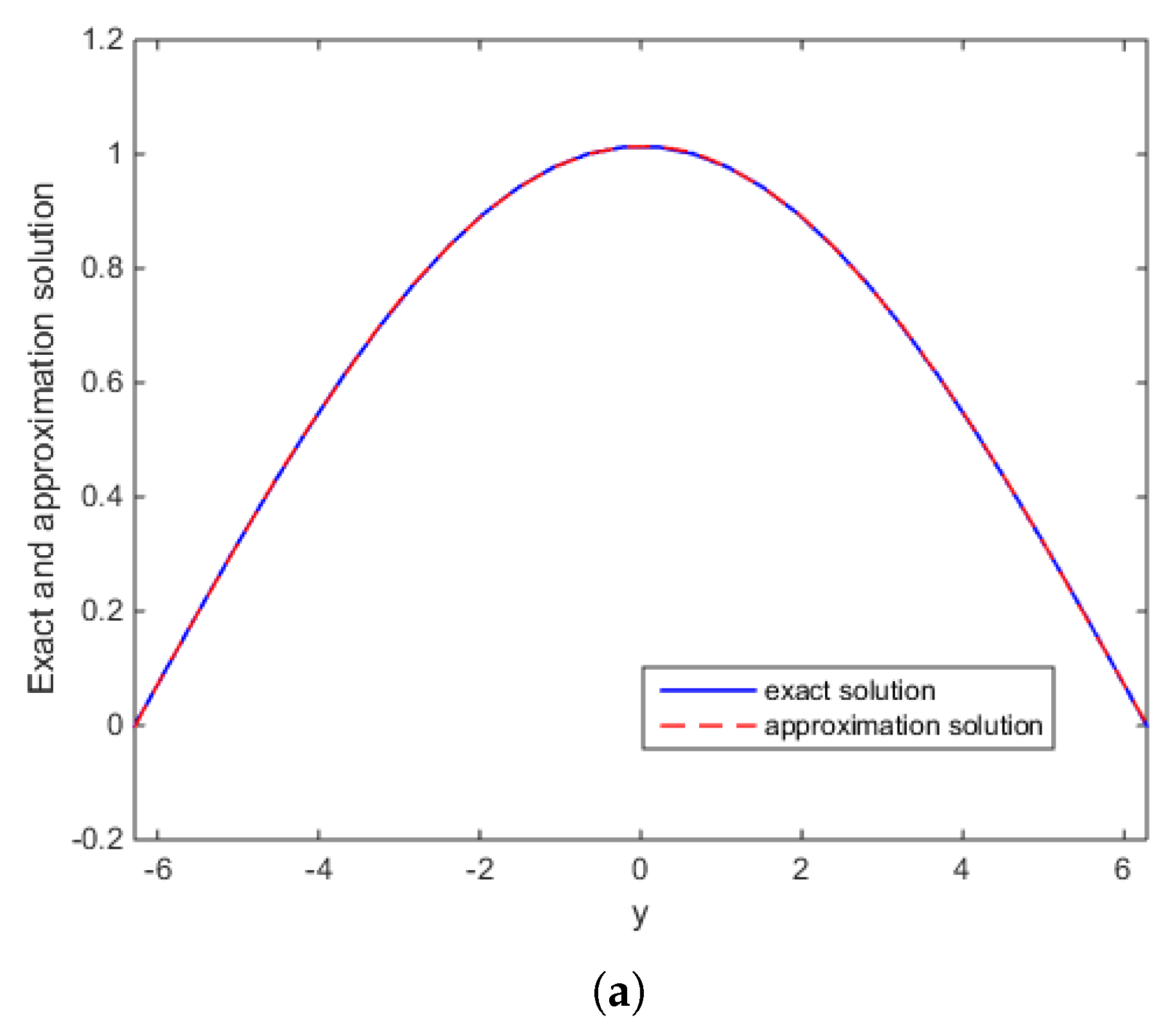
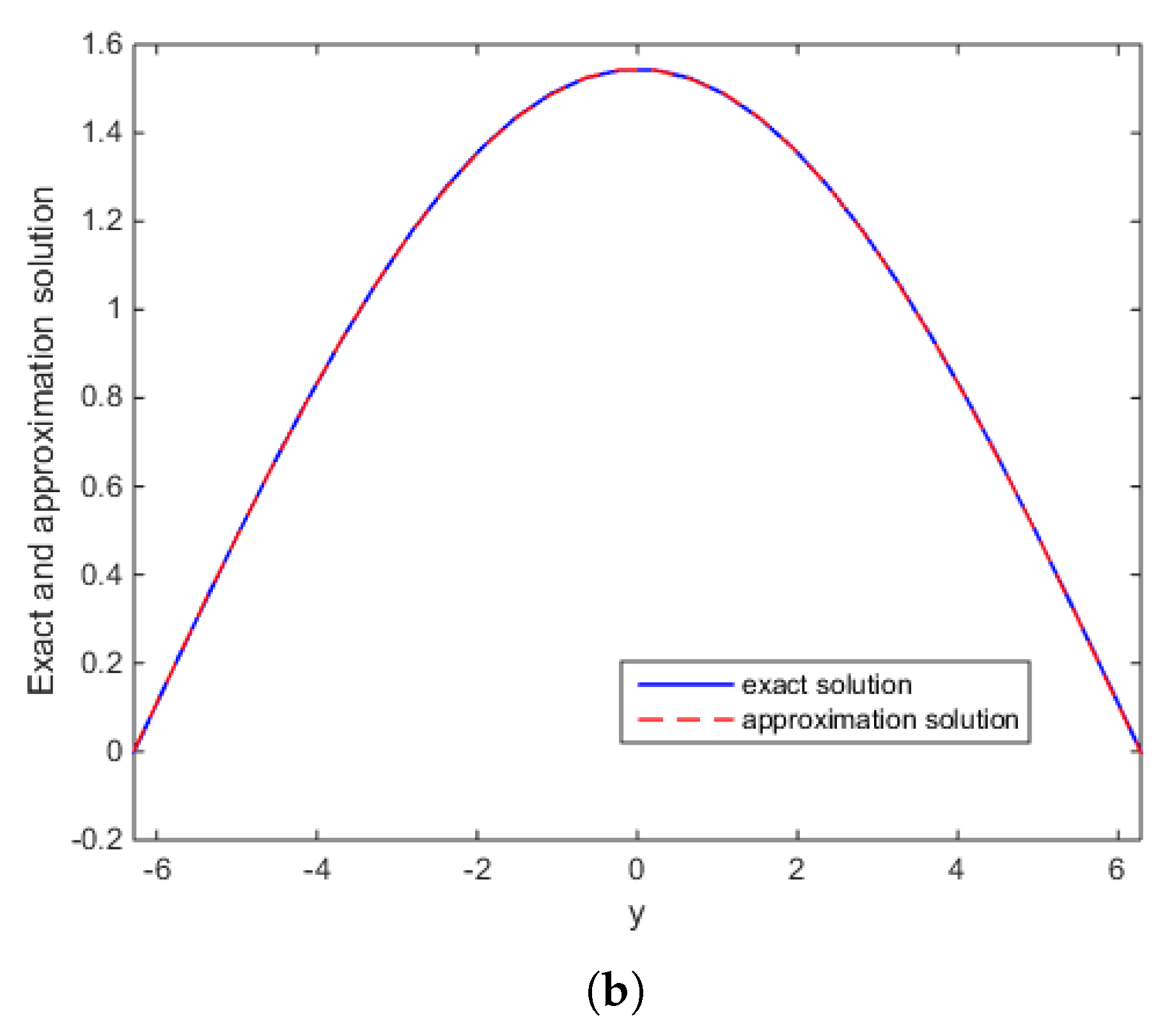
Example 1.

It’s easy to verify that function

$$v(x,y)=\frac{sin(y/2)sinh\left(x\sqrt{1/4+k^2}\right)}{\sqrt{1/4+k^2}}$$

is the exact solution of problem (2), where $g\left(y\right)=sin\left(y\right)$.

Example 2.

Apparently, the function

$$u(x,y)=cos(\frac{y}{4})cosh(x\sqrt{\frac{1}{16}+k^2})$$

is the exact solution of problem (1), where $f\left(y\right)=cos\left(\frac{y}{4}\right)$.

To verify the stability of our method, different noisy levels for $\delta =1\times {10}^{-3},1\times {10}^{-4},1\times {10}^{-5}$, $1\times {10}^{-6}$ are presented, respectively.

Table 1. The relative error $rel\left(v\right)$ of Example 1.

$\mathit{\delta }$	$1\times {10}^{-3}$	$1\times {10}^{-4}$	$1\times {10}^{-5}$	$1\times {10}^{-6}$
$rel\left(v\right)$$(k=0.5)$	0.2394	0.2397	0.2399	0.1238
$rel\left(v\right)$$(k=3)$	0.2011	0.2010	0.2008	0.2428

and

Table 2. The relative error $rel\left(u\right)$ of Example 2.

$\mathit{\delta }$	$1\times {10}^{-3}$	$1\times {10}^{-4}$	$1\times {10}^{-5}$	$1\times {10}^{-6}$
$rel\left(u\right)$$(k=0.5)$	0.001545	0.0001602	0.0001203	0.1038
$rel\left(u\right)$$(k=3)$	0.001383	0.0002011	0.07417	0.5989

show the results associated with different error levels $\delta$ of Example 1 and 2. Note that the relative error depends not only on error level $\delta$ but also on wave number k. However, due to the characteristic of the selected parametric formula, the numerical results show that the optimal range of error level within ${10}^{-5}$ and ${10}^{-3}$.

Figure 1 shows the reconstructed solution and exact solution for Example 1 corresponding to noise levels $\delta =1\times {10}^{-6}$, $\delta =1\times {10}^{-3}$ with $k=0.8$ and $k=10$, respectively. Figure 2 shows the reconstructed solution and exact solution for Example 2 corresponding to noise levels $\delta =1\times {10}^{-3}$ with $k=0.8.$ and $k=5$. Note that the proposed method is effective and stable to noisy data.

Remark 2.

In above two examples, the value of wave number k which we take is relatively small. In fact, when $k\in [0,10]$, the result is still valid, when $k>10$, the relative error will gradually increase, and the fitting effect will become more and more undesirability. Moreover, if we take N to be odd, there will be singularities, in this case, instead of $[-2\pi ,2\pi ]$, we consider interval $[-2\pi -eps,2\pi +eps]$, where $eps={10}^{-8}$ is the number of disturbance.

5. Conclusions

In this paper, a mollification method with the de la Vallée kernel for solving a Cauchy problem of the Helmholtz-type equation in a strip domain is proposed; the stable approximate estimates are obtained. Two numerical examples are investigated, and the relative errors between the regularization solution and the exact solution are presented. The numerical examples do verify the numerical efficiency and stability of our method. Furthermore, the accuracy of the procedure is quite acceptable, if noise levels are within ${10}^{-5}$ and ${10}^{-3}$.

However, the selection of regular parameters in this paper depends on the given function. In fact, we always obtain discrete data onto observation, the formulas for calculating parameters $\alpha$ in this paper are no longer applicable. At this time, we use the Golden Section Search method to calculate parameters $\alpha$, which we will use in later papers.

References

1. Wang, Y.F.L. Computational Methods for Applied Inverse Problems; Anatoly, G., Yang, C., Eds.; Higher Education Press: Beijing, China, 2012; pp. 30–72. ISBN 9787040344998. [Google Scholar]
2. Bayliss, A.; Goldstein, C.; Turkel, E.T. An iterative method for Helmholtz equztion. J. Comput. Phys. 1983, 49, 443–457. [Google Scholar] [CrossRef]
3. Benamou, J.D.; Desprès, B.T. A domain decomposition method for the Helmholtz equation and related optimal control problems. J. Comput. Phys. 1996, 6, 1–30. [Google Scholar] [CrossRef]
4. Ihlengurg, F.; Babuska, I.T. Finite element solution of the Helmholtz equation with high wave number Part two: The h-p version of the FEM. Siam J. Numer. Anal. 1997, 34, 315–358. [Google Scholar] [CrossRef]
5. Hadamard, J.L. Hep Word’s Classics. In Lectures on the Cauchy’s Problem in Linear Partial Differential Equations; Yale University Press: New Haven, CT, USA, 2007; pp. 10–120. ISBN 9787040448047. [Google Scholar]
6. Kirsch, A.L. An Introduction to the Mathematical Theory of Inverse Problems, 2nd ed.; Applied Mathematical Sciences: New York, NY, USA, 2011; pp. 73–169. ISBN 978-1-4419-8473-9. [Google Scholar]
7. Marin, L.; Elliott, L.; Heggs, P.J.T. BEM solution for the Cauchy problem associated with Helmholtz-type equations by the Landerweber method. Eng. Anal. Bound Elem. 2004, 28, 1025–1034. [Google Scholar] [CrossRef]
8. Marin, L.; Elliott, L.; Heggs, P.J.T. Conjugate gradient-boudary element solution to the Cauchy problem for Helmholtz-type equations. Comput. Mech. 2003, 31, 367–377. [Google Scholar] [CrossRef]
9. Marin, L.; Lesnic, D.T. The method of fundamental solutions for Cauchy problem associated with two-dimensional Helmholtz-type equations. Comput. Struct. 2005, 83, 267–278. [Google Scholar] [CrossRef]
10. Feng, X.L.; Fu, C.L.; Cheng, H.T. The Fourier regularization method for solving the Helmholtz equations. Appl. Num. Math. 2011, 59, 2625–2640. [Google Scholar] [CrossRef]
11. Yang, F.; Zhang, P.; Li, X.X.T. The truncation method for the Cauchy problem of the in homogeneous Helmholtz equation. Appl. Anal. 2017, 68, 1–14. [Google Scholar] [CrossRef]
12. Nikol’skii, S.M.L. Approximation of Functions of Several Variables and Imbedding Theorems; Springer: New York, NY, USA, 1975; pp. 34–320. ISBN 9783642657139. [Google Scholar]
13. Manselli, P.; Miller, K.T. Calculation of the surface temperature and heat flux on one side of a wall from measurements on the apposite side. Ann. Mat. Pura Appl. 1980, 123, 161–183. [Google Scholar] [CrossRef]
14. Murio, D.A.T. On the estimation of the boundary temperature on a sphere from measurements at its center. J. Comp. Appl. Math. 1982, 8, 111–119. [Google Scholar] [CrossRef] [Green Version]
15. Hào, D.N.T. A mollification method for ill-posed problems. Numer. Math. 1994, 68, 469–506. [Google Scholar] [CrossRef] [Green Version]
16. Murio, D.A.L. The Mollification Method and the Numerical Solution of Ill-Posed Problems; John Wiley and Sons Inc.: Hoboken, NJ, USA, 2011; pp. 23–56. ISBN 0471594083. [Google Scholar]
17. Cheng, H.; Feng, X.L.; Fu, C.L.T. A mollification regularization method for the Cauchy problem of an elliptic equation in a multi-dimensional case. Inverse Probl. Sci. Eng. 2010, 18, 971–982. [Google Scholar] [CrossRef]
18. Li, Z.P.; Fu, C.L.T. A mollification method for a Cauchy problem for the Laplace equation. Appl. Math. Comput. 2011, 217, 9209–9218. [Google Scholar] [CrossRef]
19. Xiong, X.T.; Shi, W.X.; Fan, X.Y. Two numerical methods for a Cauchy problem for modified Helmholtz equation. Appl. Math. Model. 2011, 35, 4915–4920. [Google Scholar] [CrossRef]
Figure 1. Example 1: The comparison of numerical effects between the exact solution and the approximate solution: (a) For the case k = 0.8 , δ = 1 × 10 6 ; (b) For the case k = 10 , δ = 1 × 10 3 .
Mathematics 07 00360 g001
Figure 2. Example 2: The comparison of numerical effects between exact solution and the approximate solution: (a) For the case k = 0.8 , δ = 1 × 10 3 ; (b) For the case k = 5 , δ = 1 × 10 3 .
Mathematics 07 00360 g002aMathematics 07 00360 g002b