A Hybrid Framework Combining Genetic Algorithm with Iterated Local Search for the Dominating Tree Problem

Abstract

Given an undirected, connected and edge-weighted graph, the dominating tree problem consists of finding a tree with minimum total edge weight such that for each vertex is either in the tree or adjacent to a vertex in the tree. In this paper, we propose a hybrid framework combining genetic algorithm with iterated local search (GAITLS) for solving the dominating tree problem. The main components of our framework are as follows: (1) the score functions $Dscore$ and $Wscore$ applied in the initialization and local search phase; (2) the initialization procedure with restricted candidate list (RCL) by controlling the parameter to balance the greediness and randomness; (3) the iterated local search with three phases, which is used to intensify the individuals; (4) the mutation with high diversity proposed to perturb the population. The experimental results on the classical instances show that our method performs much better than the-state-of-art algorithms.

1. Introduction

Let $G=(V,E,W)$ be an undirected, connected and edge-weighted graph, where V is the set of vertexes, E is the set of edges, and W is a non-negative weight function $E\to {\mathbb{R}}^{+}$ associated with edges. We shall use $w_{uv}$ to represent a non-negative weight of each edge $(u,v)\in E$. A tree of graph G is called dominating tree ($DT$) if each vertex in $V\backslash DT$ is adjacent to at least one vertex in $DT$. The dominating tree problem (DTP) aims to find a dominating tree $DT$ of G with the minimum total edge weight.

The DTP has many applications in real-word domains [1,2,3,4,5], such as network design and network routing in the area of wireless sensor networks (WSNs). For example, the goal of multicasting is to simultaneously transmit same message to a group of target computers [1,5]. If the edge weight represents the energy to transfer message from one server to another, the total edge weight in $DT$ equals the total cost of transferring message for multicasting. Another example is that DTP can be modelled using for routing the virtual backbone [4]. In fact, the energy cost of each edge directly affects the energy cost of the routing. Therefore, minimizing the energy cost of the routing must be considered.

The DTP has been proved to be non-deterministic polynomia-hard (NP-hard) in general [1]. At present, many different algorithms have been proposed accordingly for DTP. These algorithms can be divided into two categories (i.e., exact algorithms and heuristic algorithms) in terms of the solution method. To the best of our knowledge, there are two exact algorithms proposed in the literature for solving the DTP. In [6], Eduardo et al. proposed a solution framework combining a primal-dual heuristic with an exact branch-and-cut approach to solve DTP. The highlight of it is to transform the DTP into a Steiner tree problem for further solution. Meanwhile, Adasme et al. [7] proposed an extended version of a primal-dual model to solve DTP. In addition, they designed the effective inequalities to improve linear relaxation of the primal-dual model. In recent years, many heuristic algorithms have been proposed to solve DTP. Shin et al. [1] proposed an approximation framework with polynomial time complexity $(|v{|}^{O(lg|v|)})$ and a heuristic algorithm with low time complexity for DTP. Sundar and Singh [2] proposed two heuristic algorithms to solve DTP, viz. artificial bee colony(ABC) algorithm and an ant colony optimization (ACO) algorithm. Their algorithms are the first metaheuristic algorithms to solve DTP. Sundar [3] proposed a steady-state genetic algorithm (SSGA) to solve DTP. He designed the effective crossover and mutation operator to improve the performance of SSGA. Dražić et al. [5] proposed a variable neighborhood search (VNS) approach to solve DTP. They properly used the arrangement of vertex sets in the neighborhood structure and the local search phase. At the same time, Chaurasia and Singh [4] proposed an evolutionary algorithm which employs a guided mutation (EA/G) operator to solve DTP. It tried to overcome the shortcomings of genetic algorithms. Sundar and Singh [8] proposed a novel artificial bee colony algorithm (ABC_DT) to solve DTP. ABC_DT is different from existing ABC on two main points, viz. initial phase and the acquisition of the neighborhood solution. Although many heuristic algorithms have been proposed to solve DTP, there is still room for improvement based on these existing results.

Tremendous work on the memetic search has been done by more and more researchers due to its effectiveness and adaptiveness [9,10,11,12,13,14]. It is essentially a combination of a global search based on population and a local search based on individuals. In this framework, different memetic search can be constructed using different search strategies. For example, global search strategies can use genetic algorithms, evolution strategies, etc. Local search strategies can use simulated annealing, greedy algorithm, tabu search, etc. Tang et al. [9] proposed a memetic algorithm with extended neighborhood search for the capacitated arc routing problem (CARP). They mainly designed an effective local search approach to increase search space and diversity. Kannan et al. [10] proposed a novel memetic framework combining a genetic algorithm with local search-based filter ranking. Wang et al. [11] proposed a novel memetic algorithm based on tabu search for the maximum diversity problem (MDT). Tabu search phase effectively used continuous filtering candidate list strategy. In this paper, our proposed algorithm shall make full use of the advantages of the local search framework and genetic algorithm.

In this paper, we propose an effective hybrid framework combining genetic algorithm with iterated local search for DTP. Firstly, we design two functions $Dscore$ and $Wscore$ which are used to help make the decisions on which vertex should be added to or removed from the solution. Secondly, the initialization procedure with RCL ($Init\_RCL$) is proposed to initialize the population. By controlling the parameter $\alpha$, $Init\_RCL$ can balance the greediness and randomness to some extent. Third, the iterated local search ($ITLS$) including three phases is applied to intensify the individuals in the population. In the removing phase, some vertexes with higher $Dscore$ are removed, and the dominating phase and connecting phase are applied to repair the solution greedily considering the $Dscore$ and $Wscore$. Due to the high greediness in the $ITLS$, a mutation with high diversity is performed to perturb the population. Some vertexes are randomly removed, then we also use the same procedure in $ITLS$ to repair the solution. Finally, the framework is outlined. We shall compare our proposed algorithm with the state-of-the-art heuristic algorithms, viz. VNS and ABC_DT. The experimental results show that our algorithm performs much better than VNS and ABC_DT on the classical benchmark instances.

The structure of our paper is as follows. Some basic concepts are provided in Section 2. In Section 3, we introduce our framework and its components including the score function, the initialization procedure, the iterated local search and the mutation with high diversity. The experimental results are shown in Section 4. Finally, we summarize our work and put forward some new ideas for the future work in Section 5.

2. Preliminaries

Let $G=(V,E,W)$ be an undirected, connected and edge-weighted graph, where V is the set of vertexes, E is the set of edges, and W is a non-negative weight function $E\to {\mathbb{R}}^{+}$ associated with edges. We shall use $w_{uv}$ to represent a non-negative weight of each edge $(u,v)\in E$. We shall use $hop(u,v)$ to denote the number of edges in a shortest hop path (not considering the edge weight) from u to v. Then, $N^i(v)=\{u|hop(u,v)=i\}$ is used to present the ith level neighbors of the vertex v. In addition, we denote $N^i[v]=N^i(v)\cup \{v\}$. Particularly, $N(v)$ is the neighbor set of v and $N[v]$ also includes the v itself except $N(v)$. Some definitions are described as follows.

Definition 1.

(Induced Subgraph, IS) Given an undirected graph $G(V,E)$, $G^{\prime }=(V^{\prime },E^{\prime }),V^{\prime }\subseteq V,E^{\prime }=\{(u,v)|(u,v)\in E,u,v\in V^{\prime }\}$, subgraph $G^{\prime }$ is called the induced subgraph of graph G.

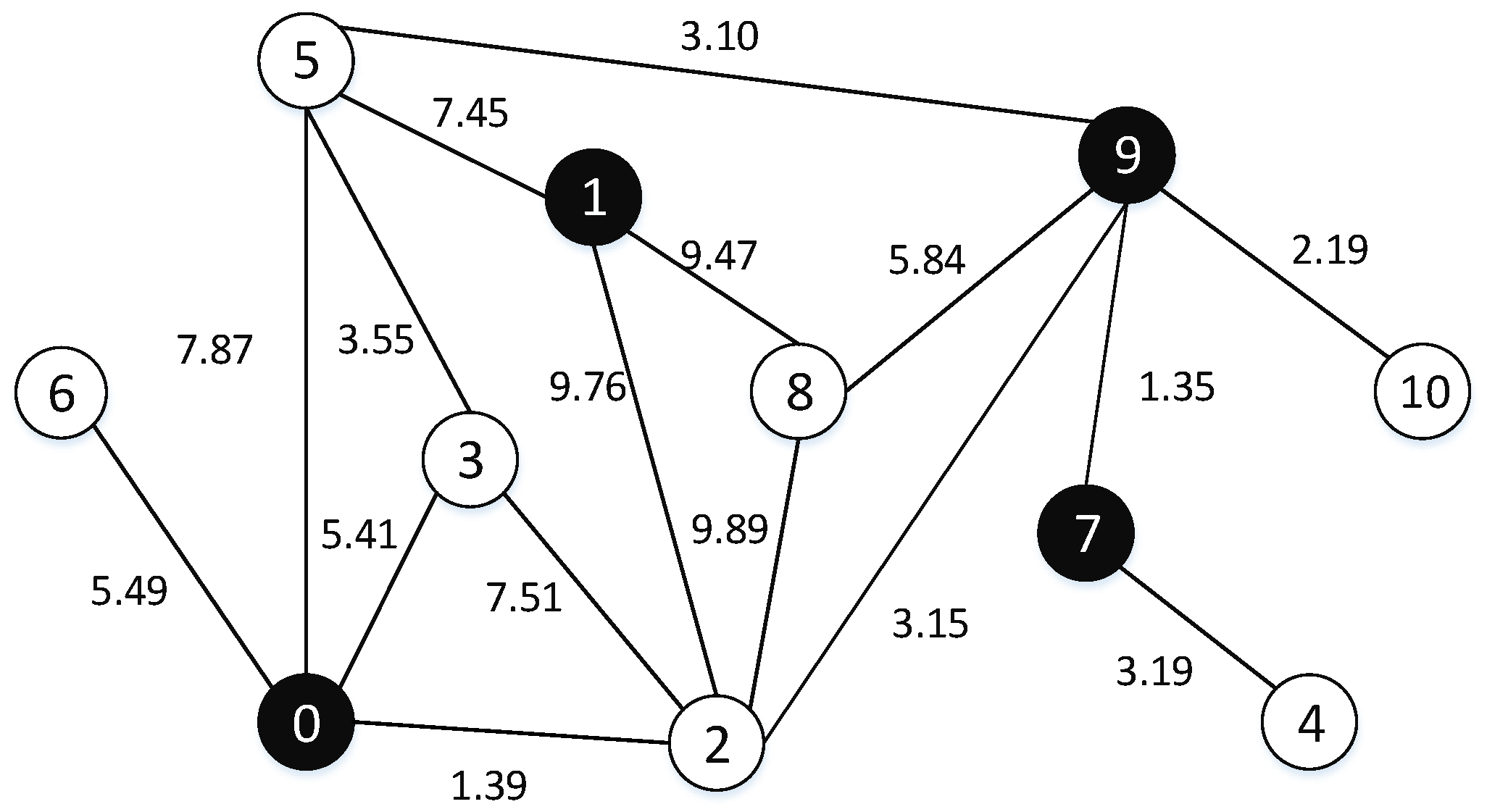
Definition 2.

(dominating set, DS) Given an undirected graph $G(V,E)$, the dominating set of G is a vertex subset $D\subseteq V$ such that every vertex in V\D has at least one neighbor in D. (An example is shown in Figure 1).

Definition 3.

(minimum dominating set, MDS) Given an undirected graph $G(V,E)$, the minimum dominating set problem calls for finding a dominating set D with minimum cardinality.

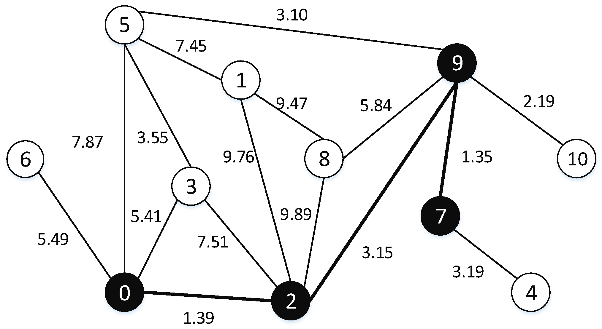
Definition 4.

(Dominating tree problem, DTP) Given an undirected and edge-weighted graph $G=(V,E,W)$, the $DTP$ calls for finding a tree with minimum total edge weight such that every vertex in V\DT has at least one neighbor in $DT$. (An example is shown in Figure 2).

Figure 1 and Figure 2 show an undirected graph G with 11 vertexes and 16 edges. The black vertexes are in the dominating set, hence in Figure 1 {0, 1, 7, 9} is a dominating set of G. In Figure 2, the black vertexes (viz. 0, 2, 7, 9) are in $DT$ and the edges of the minimum spanning tree are the bold. The total edge weight of the dominating tree is 5.89. We can observe that {0, 2, 7, 9} is also a dominating set of G. It embodies that the dominating tree satisfies the characteristic of the dominating set.

3. The Hybrid Framework Combining Genetic Algorithm with Iterated Local Search for DTP

In this section, we focus on the framework proposed for solving the DTP, which is a hybrid framework by combining the genetic algorithm with iterated local search. Before providing the framework, the score functions will be introduced firstly, which will be applied in the initialization procedure and the iterated local search phase. Then, we present the initialization procedure which can balance the greediness and the randomness to some extent. Subsequently, the iterated local search is described in details, which is used to intensify the individuals in the population. In order to maintain the diversity of the individuals, we utilize the mutation to perturb the population. Finally, the hybrid framework combining the genetic algorithm with iterated local search (GAITLS) is presented.

3.1. The Score Functions

To guide the search toward the direction with more possible best solutions, the score function is designed to help the search make the decision on selecting the vertex to add to or remove from the solution. Lots of score functions have been proposed in [15,16,17,18] for the different problems. Considering the features of DTP, we design the $Dscore$ and $Wscore$ function which will be applied in two phases including the iterated local search and the initialization. How to apply the $Dscore$ and $Wscore$ is introduced in the following subsections. Now we give the information about $Dscore$ and $Wscore$.

• $Dscore$: For a vertex v in the solution, $Dscore$ indicates how many vertexes will become non-dominated from dominated once v is removed from the solution. That is to say, $Dscore$ is equal to the number of neighbors of v which are only dominated by v. If the vertex v is not in the solution, $Dscore$ represents how many vertexes will become dominated from non-dominated once v is added to the solution. In this case, $Dscore$ is equal to the number of neighbors of v which are non-dominated. The definition of $Dscore$ is listed as follows.

  $$Dscore[v]=\left\{\begin{array}{c}-1\times |\{u|u\in N[v]anduisonlydominatedbyv\}|,v\in DT\hfill \\ |\{u|u\in N[v]anduisnondominated\}|,v\notin DT\hfill \end{array}\right.$$

  (1)
  In order to distinguish between the vertexes $v\in DT$ and $v\notin DT$, the $Dscore$ value of $v\in DT$ is non-positive by times −1. Once one vertex is added to or removed from the $DT$, we do not need re-compute the $Dscore$ for each vertex and we just need update the $Dscore$ of $N[v]$ and $N^2[v]$.
• $Wscore$: For each vertex not in the solution $DT$, we design the $Wscore$ function to evaluate the effect on the final sum weight of edges in the minimum spanning tree if one vertex is added to $DT$. The definition of $Wscore$ is listed in Equation (2). The $SP(v,v^{\prime })$ means the shortest path between $v\notin DT$ and $v^{\prime }\in DT$. $Wscore[v]$ is equal to the minimum over all such shortest paths $SP(v,v^{\prime })$. The shortest path for each vertex pair has been computed in the preprocessing phase, so it is easy to update the $Wscore[v]$ for each vertex not in $DT$.

  $$Wscore[v]=\underset{v^{\prime }\in DT}{min}SP(v,v^{\prime }),v\notin DT$$

  (2)

3.2. The Initialization Procedure

For the evolutionary algorithm, the important component is the population. The quality of the population has an important impact on the final results. Generally, the population should be balanced considering the greediness and randomness. Greediness is used to guarantee the individuals with better objective while the randomness is used to guarantee the diversity of population on the whole. Hence, we adopt the restricted candidate list (RCL) to initialize the population. RCL can control the greediness strength by the parameter and has been widely applied to solve the combinational optimization problem [18,19,20].

The initialization procedure ($Init\_RCL$) is outlined in Algorithm 1. The inputs are the graph $G(V,E,W)$, the size of population $IndiNum$, and the parameter $\alpha$ which is used to control the greediness strength. The bigger the $\alpha$, the stronger the greediness. In order to save time, we compute the shortest path for each vertex pair in the preprocessing phase. Then, the procedure generates $IndiNum$ individuals to construct the population by executing a series of iterations. At each iteration, one individual is produced. To start with, the solution $DT$ is initialized to the empty set. In order to guarantee the solution is connected, we maintain a candidate list (CL) which is used to store the neighbors (not in $DT$) of the vertexes in $DT$. $CL$ is initialized to empty set due to no vertex in the $DT$. Then, the $Dscore[v]$ is initialized to $|N[v]|$. One vertex will be randomly selected from RCL to add to the $DT$ at each inner iteration. Therefore, firstly we need to construct the $RCL$. For the first vertex, we just consider the $Dscore$. The $maxscore$ and $minscore$ represent the maximum and minimum value of $Dscore$ over the vertexes in V. The vertexes with $Dscore$ greater than or equal to $minscore+\alpha \times (maxscore-minscore)$ will be added to the RCL. For the remaining vertexes, we will consider the weight of edges connecting to the vertexes in $DT$. The $maxscore$ and $minscore$ represent the maximum and minimum value of $Dscore[v]/min(w_{uv})$ over vertexes in $CL$, where $min(w_{uv})$ is the minimum weight of edges connecting v to the vertex u in $DT$. After randomly selecting a vertex $AddVertex$ from $RCL$, some information should be updated, such as the $CL$, $DT$ and $Dscore$ of $N[AddVertex]$ and $N^2[AddVertex]$. The inner loop will stop until the there is no non-dominated vertex indicating the individual is a feasible solution.

Once an individual is constructed, we will execute the pruning procedure to remove the redundant vertexes [2]. Subsequently, we connect the vertexes in $DT$ by constructing the minimum spanning tree with the help of Prim’s algorithm [21]. In addition, the fitness of the individual is equal to the sum weight of edges in the spanning tree. Finally, the new individual will be inserted into the population $PO{P}_{init}$. The outer loop will stop until the population is full.

3.3. The Iterated Local Search Based on the Dynamic Score Functions

In each generation, we apply the iterated local search (ITLS) to intensify the individuals. During the ITLS, we use the score functions introduced above to lead the direction toward the solutions with more possible best solutions. The framework of ITLS is described in Algorithm 2.

The graph $G(V,E,W)$ and the current solution $DT$ are as the inputs for the ITLS. In addition, ITLS will return the local best solution $D{T}^{\prime }$ which is initialized to $DT$. Before performing the iteration, we need compute the $Dscore[v]$ for each vertex according to Equation (1). Subsequently, a series of iterations are executed to improve the current solution $DT$. Here, we use the max iterations as the stop criterion. At each iteration, we firstly judge whether the current solution is feasible. If that, we will perform the pruning phase by removing the redundant vertexes and connect the vertexes in $DT$ by constructing the minimum spanning tree. If the $DT$ is better than $D{T}^{\prime }$, $D{T}^{\prime }$ will be updated.

Then, three phases are followed. (1) In the removing vertexes phase, we always remove the vertex with the highest $Dscore[v]$ value from $DT$ until there exists non-dominated vertex. Meanwhile, the removed vertex should be not in tabul_list to avoid the search to meet the same situation quickly. Here, we use the simple tabu_list and the vertex added at the last iteration is not allowed to be removed at the current iteration. To guarantee the solution feasible, we do not use the tabu list when adding the vertex to the solution. If there are more than one vertex with the highest value $Dscore$, we prefer to the vertex in $DT$ longer time evaluated by how many iterations the vertex has not changed the state (in or not in DT). Once a vertex is removed, the $Dscore$ of $N[v]$ and $N^2(v)$ should be updated. The following two phases are applied to repair the infeasible solution. (2) In the dominating phase, we add some vertexes to $DT$ until $DT$ is a dominating set. When selecting the vertex, we consider the $Dscore$ meaning how many vertexes will become dominated after adding the vertex. We also consider the effect $Wscore[v]$ on the weight of edges connecting v with the vertexes in $DT$. $Wscore[v]$ is equal to the minimum over the shortest paths from v to the vertexes in $DT$. Therefore, the vertex with lowest $Wscore[v]/Dscore[v]$ is selected to add to $DT$. (3) In the connecting phase, we compute all the shortest paths between the vertexes in different components. The shortest path is chosen and the vertexes along the path are added to the solution. The procedure will continue until there is only one component. Finally, the tabu list and the $Dscore$ are updated.

Algorithm 1: The initialization procedure ($Init\_RCL$).

Algorithm 2: The iterated local search based on the score functions (ITLS).

3.4. The Mutation with High Diversity

Generally, the genetic algorithm uses the crossover to combine the genetic information of two parents and pass down the excellent genes to the offspring. However, for the DTP problem the crossover usually leads to the same offspring. Therefore, we adopt the mutation with high diversity to improve the situation. The ITLS focuses on one solution and greedily to explore the solution space. In order to explore bigger space, we use the mutation to perturb the parent solution and generate the offspring.

During the ITLS, we always remove the vertexes with the highest $Dscore$, which may lead the search to trap in the local optima. Hence, some vertexes are randomly selected to remove from the solution in the mutation phase until the solution is not a dominating set. After removing the vertex, the solution is infeasible and we conduct two phases including dominating and connecting phase like in ITLS to repair it. The difference is that we do not apply the tabu list in the mutation phase. Furthermore, the new solution generated by the mutation will replace the parent solution no mater whether it is better than parent or not. The reason is that after ITLS the individual is replaced by the local optima. The best solution $D{T}^{*}$ will be updated if the offspring is better than $D{T}^{*}$.

3.5. The Hybrid Framework Combining Genetic Algorithm with Iterated Local Search (GAITlS)

After introducing the components respectively, we provide the framework in this section, which is shown in Algorithm 3.

The inputs of GAITLS include the graph $G(V,E,W)$, the size of population $IndiNum$, the cut-off time and the greediness strength $\alpha$ for the initialization procedure. To start with, the population $POP$ is initialized by calling the procedure $InitRCL(G,IndiNum,\alpha )$. Then, $D{T}^{*}$ is initialized to the individual with the best objective in $POP$. The outer loop (line 3–15) will continue until the the elapsed time is greater the cut-off time. At each generation, the iterated local search is performed for each individual in the population (line 6–10). The individual is replaced by the solution returned by ITLS. Once the better solution is found during the ITLS, the best solution $D{T}^{*}$ will be updated. After the ITLS, for each individual we perform the mutation to increase the diversity. The best solution $D{T}^{*}$ also will be updated during the mutation phase.

Algorithm 3: The hybrid framework combining genetic algorithm with iterated local search (GAITLS).

4. Experiments

In this section, we carry out plentiful experiments to evaluate the efficiency of our algorithm on standard benchmarks. We have compared our proposed algorithm with the state-of-the-art heuristic algorithms, viz. VNS and ABC_DT. In our experiments, there are two classic benchmark instances, dtp and range, which can be downloaded from the webpage [22]. For each instance of dtp, $|V|\in \{10,15,20,100,200,300\}$ and $|E|\in \{15,20,30,50,150,200,400,600,1000\}$. For each instance of range, $|V|\in \{50,100\}$ and three values of transmission range, viz. 100, 125 and 150. It should be noted that, VNS is the best heuristic algorithm on dtp benchmark, and ABC_DT is the best heuristic algorithm on range benchmark. Our algorithm will compare with VNS and ABC respectively.

Our proposed algorithm is implemented in C++ and compiled by g++ with the -O2 option. All computational experiments were performed on the Linux Ubuntu with Intel(R) Xeon(R) CPU E7-4830 @2.13Ghz and 8GB memory. It should be noted here that ABC_DT and VNS are implemented in C [5,8]. Our proposed algorithm run 20 times independently for each instance with different random seeds, until the time limit (600 s) is satisfied. In our algorithm, it is important to make appropriate adjustments to the parameters. There are mainly three parameters values(viz. $IndiNum$ = 50, $\alpha$ = 0.85, $step$ = 1,000,000) where are determined by performing a preliminary experiment. $IndiNum$ presents the size of the population, and $\alpha$ presents the greediness strength when constructing the RCL. $step$ is used to control the number of iterations in the local search phase.

4.1. Computational Results

In the results of our experiment, $Best$ presents the best solution values, $Avg$ presents the average solution values, and $AvgTime$ presents the average run time to reach the best solution. Note that the bold value presents the best solution value among the different algorithms compared (in terms of $Best$ and $Avg$). $Opt$ presents the optimal solution which is acquired by two exact algorithms [6,7]. $Init$ represents the initial solution obtained by GAITLS. For some instances, exact algorithm failed to find a optimal solution, then it is marked as “$na$” for these cases.

The experimental results of algorithms are shown in

Table 1. Experimental results of VNS and GAITLS on small size instances of dtp.

			VNS			GAITLS
Instances	Opt	Best	Avg	AvgTime		Init	Best	Avg	AvgTime
dtp_10_15_0	5.89	5.89	5.89	0.04		5.89	5.89	5.89	0
dtp_10_15_1	14.42	14.42	14.42	0.04		14.42	14.42	14.42	0
dtp_10_15_2	14.35	14.35	14.35	0.04		16.72	14.35	14.35	0
dtp_15_20_0	18.87	18.87	18.87	0.1		22.65	18.87	18.87	0
dtp_15_20_1	23.03	23.03	23.03	0.09		29.84	23.03	23.03	0
dtp_15_20_2	24.95	24.95	24.95	0.1		29.11	24.95	24.95	0
dtp_15_30_0	18.2	18.2	18.2	0.11		19.7	18.2	18.2	0
dtp_15_30_1	8.32	8.32	8.32	0.08		8.32	8.32	8.32	0
dtp_15_30_2	18.07	18.07	18.07	0.09		23.21	18.07	18.07	0
dtp_20_30_0	33.81	33.81	33.81	0.22		38.39	33.81	33.81	0
dtp_20_30_1	36.03	36.03	36.03	0.2		41.73	36.03	36.03	0
dtp_20_30_2	43.5	43.5	43.5	0.23		51.11	43.5	43.5	0
dtp_20_50_0	9.81	9.81	9.81	0.17		9.81	9.81	9.81	0
dtp_20_50_1	12.19	12.19	12.19	0.16		16.08	12.19	12.19	0
dtp_20_50_2	17.42	17.42	17.42	0.2		23.16	17.42	17.42	0

,

Table 2. Experimental results of VNS and GAITLS on large instances of dtp.

			VNS			GAITLS
Instances	Opt	Best	Avg	AvgTime		Init	Best	Avg	AvgTime
dtp_100_150_0	152.57	152.57	154.61	294.95		174.62	152.57	152.57	186.2
dtp_100_150_1	192.21	192.21	194.22	286.39		210.8	192.21	192.21	0
dtp_100_150_2	146.34	146.34	148.35	245.61		154.66	146.34	146.34	0.06
dtp_100_200_0	135.04	135.04	136.41	333.91		167.1	135.04	135.04	61.29
dtp_100_200_1	91.88	91.88	92.03	133.19		126.45	91.88	91.88	0
dtp_100_200_2	115.93	115.93	117.11	372.14		125.66	115.93	115.93	0.34
dtp_200_400_0	257.09	306.06	343.95	565.14		310.67	257.09	257.09	82.77
dtp_200_400_1	258.77	303.53	331.1	559.42		311.48	258.93	258.93	413.3
dtp_200_400_2	238.27	274.37	289.51	550.36		278.42	238.29	238.29	23.32
dtp_200_600_0	121.62	132.49	150.39	553.69		156.37	121.62	121.62	194
dtp_200_600_1	135.08	162.92	198.21	556.62		170.37	135.08	135.08	1.62
dtp_200_600_2	123.31	139.08	154.36	520.87		159.21	123.31	123.31	7.1
dtp_300_600_0	348.03	471.69	494.62	538.95		398.76	348.03	348.03	479.49
dtp_300_600_1	413.93	494.91	542.46	544.27		466.84	415.32	415.32	61.53
dtp_300_600_2	352.15	500.72	535.3	533.8		398.46	358.53	358.53	10.31
dtp_300_1000_0	na	257.72	264.33	575.1		201.76	149.57	149.57	470.12
dtp_300_1000_1	na	242.79	325.16	530.51		231.97	165.19	165.19	312.21
dtp_300_1000_2	na	223.18	251.41	482.59		202.25	154.61	154.61	7.64

and

Table 3. Experimental results of ABC_DT and GAITLS on instances of range.

			ABC_DTP			GAITLS
Instances	Opt	Best	Avg	AvgTime		Init	Best	Avg	AvgTime
R100_50_1	1024.41	1204.41	1204.41	0.44		1286.31	1024.41	1024.41	0.06
R100_50_2	1340.44	1340.44	1340.69	0.64		1398.51	1340.44	1340.44	6.17
R100_50_3	1316.39	1316.39	1316.39	0.56		1399.71	1316.39	1316.39	2.56
R100_100_1	1217.47	1217.47	1218.59	1.11		1273.02	1217.47	1217.65	293.83
R100_100_2	1128.4	1128.4	1136.5	1.12		1281.33	1128.4	1128.4	15.1
R100_100_3	1252.99	1252.99	1253.3	1.2		1351.87	1252.99	1252.99	279.04
R125_50_1	802.95	802.95	802.95	0.24		827.44	802.95	802.95	0.01
R125_50_2	1055.1	1055.1	1055.1	0.32		1149.88	1055.1	1055.1	1.02
R125_50_3	877.77	877.77	877.83	0.32		941	877.77	877.77	0.13
R125_100_1	943.01	943.01	943.01	0.77		1010.95	943.01	943.01	82.89
R125_100_2	917	917	917.38	0.71		1030.15	917	917.22	196.02
R125_100_3	998.18	998.18	999.91	1.06		1080.4	998.18	998.18	6.76
R150_50_1	647.75	647.75	647.75	0.19		666.08	647.75	647.75	3.04
R150_50_2	863.69	863.69	864.04	0.27		925	863.39	863.39	0.59
R150_50_3	743.94	743.94	745.68	0.18		847.22	743.94	743.94	49.07
R150_100_1	876.69	876.69	877.02	0.57		985.28	876.69	876.69	14.28
R150_100_2	657.35	657.35	657.53	0.66		727.84	657.35	659.35	108.41
R150_100_3	722.87	722.87	722.87	0.54		730.37	722.87	722.87	0.27

. Table 1 shows the results of VNS and our algorithm on small size instances of dtp. Compared with VNS, GAITLS can obtain the optimal solution on all instances. In addition, both the algorithms have the same average solution on all instances. Our algorithm is faster than VNS in terms of the average time of solution. Table 2 shows the results of VNS and our algorithm on large size instances of dtp. Form Table 2, our algorithm can obtain the same best values with VNS on 6 instances. In the remaining 12 instances, our algorithm can obtain better best values with VNS. In terms of $Avg$ and $AvgTime$, our algorithm is better than VNS on all instances. This shows that our algorithm has been considerably improved compared to VNS. Table 3 shows the results of ABC_DT and our algorithm on range benchmark. From Table 3, all of them can be solved to optimality. We can observe that the quality of Avg obtained by our algorithm is much better than ABC_DT with one exception, viz. R150_100_2. The computational results in Table 1, Table 2 and Table 3 show that our algorithm can be resoundingly applied to spares instances. It distinctly indicates that the combination of genetic algorithm and iterated local search in our algorithm can effectively solve DTP.

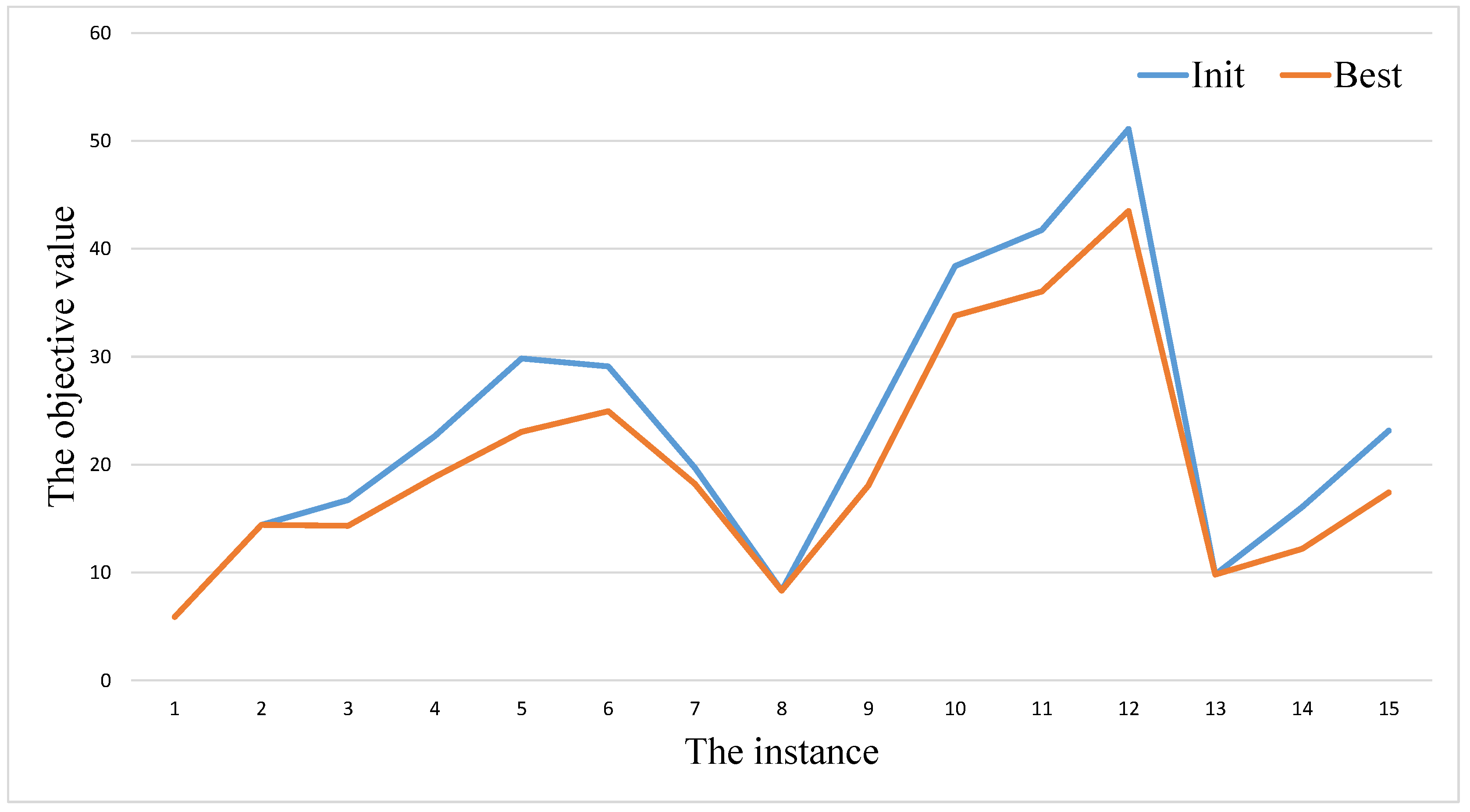
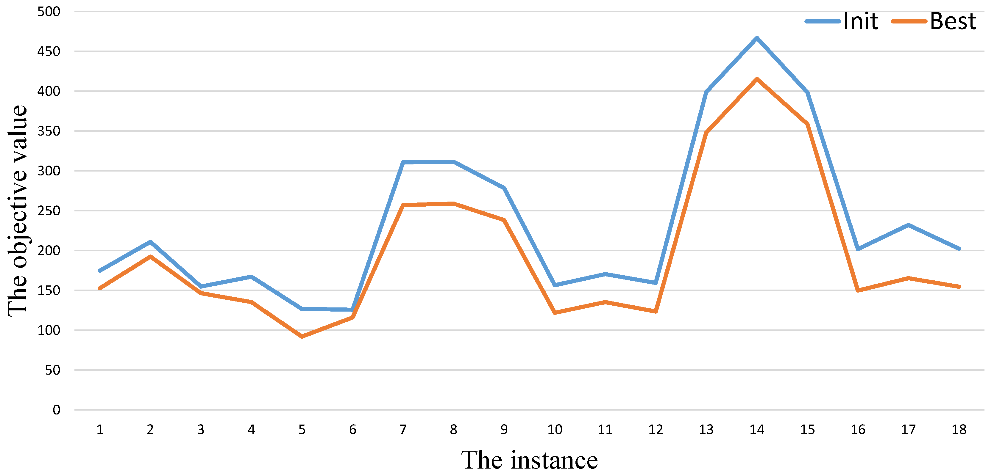
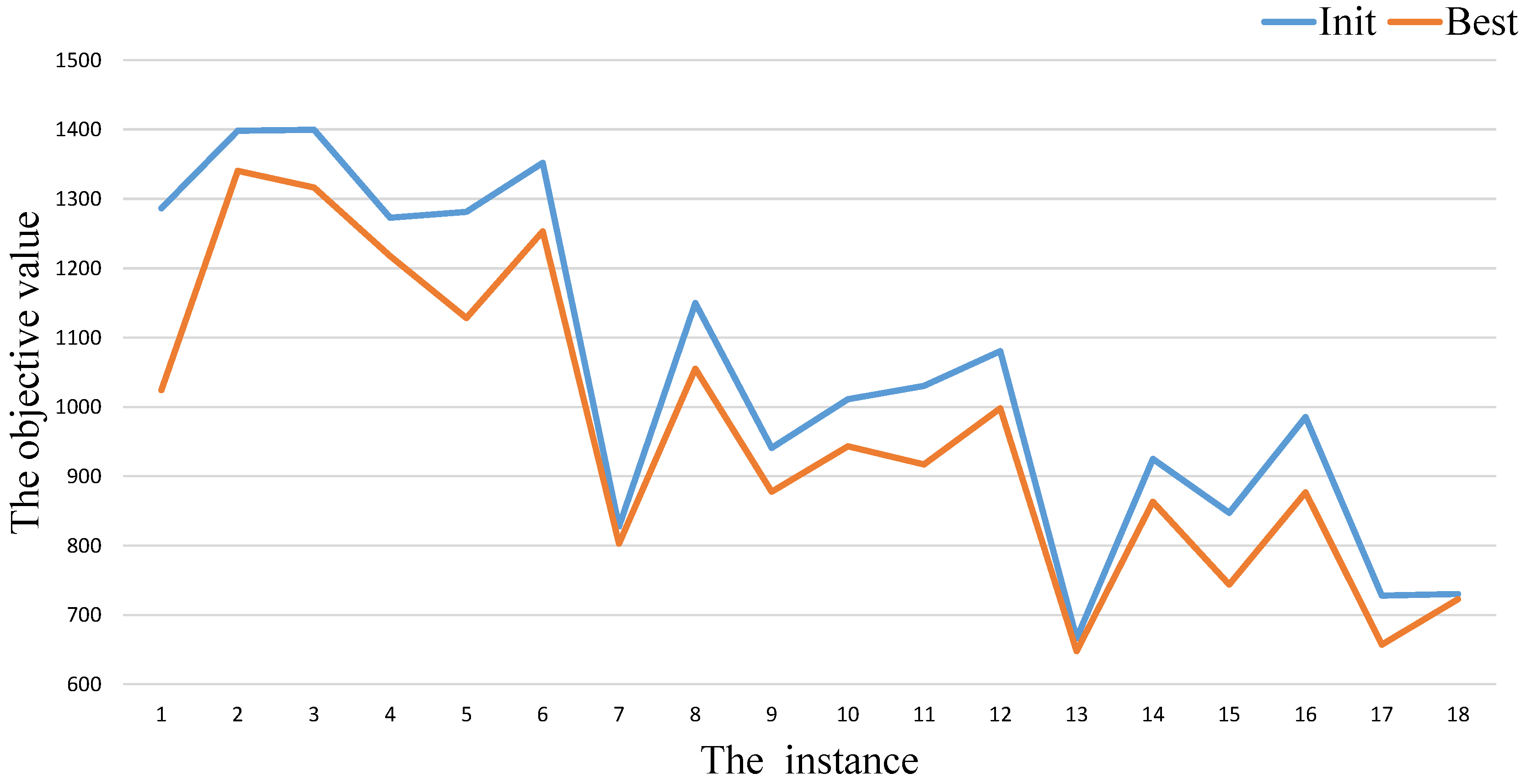
As shown in Table 1, Table 2 and Table 3, we also list the results obtained by the initialization procedure in the column Init. After calling the initialization procedure ($Init\_RCL$), we get a population. Therefore, the value of $Init$ represents the best objective value among the population over 20 independent times run. By comparing the values of the columns $Init$ and $Best$ of our algorithm GAITLS, we can find that the initialization procedure cannot get as good as the final results on almost instances in Table 1, Table 2 and Table 3. In order to show the gap intuitively, we provide Figure 3, Figure 4 and Figure 5. The blue and orange cures represent the values of the column $Init$ and $Best$ respectively. From these figures, we also can observe that there always exists gaps between $Init$ and $Best$.

4.2. Analysis and Discussion

In this section, we analyse the computational complexity of the initialization procedure (Algorithm 1) and the iterated local search (Algorithm 2). Meanwhile, we also discuss the difference between our algorithm and the comparative algorithms.

Considering the initialization procedure $Init\_RCL$, when constructing an individual at each iteration the $RCL$ need be maintained and a vertex will be selected from the $RCL$. At most $|V|$ is added to the dominating set, so the computational complexity of $Init\_RCL$ is O($|V|\times IndiNum$), where $IndiNum$ is the number of individuals in the population. Regarding the iterated local search based on the score functions (Algorithm 2), we analyse the three phases respectively. For the removing phase, the vertex with highest $Dscore$ will be removed, and the $Dscore$ of vertexes in $N[v]$ and $N^2[v]$ is updated. At most $|DT|$ vertexes can be removed, so the computational complexity is O($|DT|$). The dominating phase is similar to the removing phase and the computational complexity is O($|V\backslash DT|$). Actually, the connecting phase is with highest computational complexity which depends on the number of components. Although we have preprocessed the shortest paths, we need find the shortest path between the components. However, after the dominating phase the number of components usually is small due to small-scale of the instances.

Regarding the comparative algorithm variable neighborhood search (VNS), it randomly produces an initial solution and use the local search to improve it. For the different neighborhoods, it use different shake strength. However, the local search scan all the vertex pairs to swap, which takes long time and does not use the information of the current solution. The algorithm artificial bee colony for dominating (ABC_DT) is a swarm intelligence techniques. There is an important component in the ABC_DT, that is, the determination of a neighboring solution. The authors propose two methods for determining a solution in the neighborhood of current solution. $CNAS$-$Method$ is based on copy a set of dominating nodes from another solution of the population to current solution, whereas $MEDI$-$Method$ is based on performing random multiple $edge$-$deletion$-$insertion$ on current solution. $CNAS$-$Method$ copies the dominating nodes from another individual but does not consider the effect on the final solution. $MEDI$-$Method$ is the random phase. Therefore, we can find VNS and ABC_DT cannot the information of nodes and current solution to guide the search direction. We use the score function $Dscore$ and $Wscore$ to guide the search towards the better solution, and the mutation with high diversity is applied to increase diversity. Our algorithm GAITLS can balance the greediness and randomness.

5. Summary and Future Work

A hybrid framework combining genetic algorithm with iterated local search GAITLS is proposed for solving the dominating tree problem in this paper. Firstly, two score functions are defined, i.e., $Dscore$ and $Wscore$. $Dscore$ represents how many vertexes will change the state after adding (removing) one vertex to (from) the solution while $Wscore$ is used to evaluate the possible effect on the final sum weight of edges in the minimum spanning tree. $Dscore$ and $Wscore$ will help make the decision which vertex should be selected to add to or remove from the solution in the initialization procedure and iterated local search. Secondly, the initialization procedure with RCL ($Init\_RCL$) is presented to initialize the population. By controlling the parameter $\alpha$, $Init\_RCL$ can balance the greediness and randomness to some extent. Thirdly, the iterated local search ($ITLS$) including three main phases is provided. In the removing phases some vertexes with higher $Dscore$ are removed, and dominating phase and connecting phase are used to repair the solution greedily considering the $Dscore$ and $Wscore$. Then, the mutation with high diversity is proposed to perturb the individuals to increase the diversity. Finally, the hybrid framework is outlined. The experimental results indicate that GAITLS performs well in solving DTP.

The instances of dominating tree problem are all small-scale. We are interested in the performance of the applied methods. Therefore, we would like to design the efficient algorithm to solve DTP on the large-scale instances.