Article

Scattered Data Interpolation and Approximation with Truncated Exponential Radial Basis Function

School of Mathematics and Statistics, Ningxia University, Yinchuan 750021, China
*
Author to whom correspondence should be addressed.
Mathematics 2019, 7(11), 1101; https://doi.org/10.3390/math7111101
Submission received: 14 October 2019 / Revised: 7 November 2019 / Accepted: 11 November 2019 / Published: 14 November 2019
(This article belongs to the Special Issue Computational Mathematics, Algorithms, and Data Processing)

Abstract

:
Surface modeling is closely related to interpolation and approximation by using level set methods, radial basis functions methods, and moving least squares methods. Although radial basis functions with global support have a very good approximation effect, this is often accompanied by an ill-conditioned algebraic system. The exceedingly large condition number of the discrete matrix makes the numerical calculation time consuming. The paper introduces a truncated exponential function, which is radial on arbitrary n-dimensional space R n and has compact support. The truncated exponential radial function is proven strictly positive definite on R n while internal parameter l satisfies l n 2 + 1 . The error estimates for scattered data interpolation are obtained via the native space approach. To confirm the efficiency of the truncated exponential radial function approximation, the single level interpolation and multilevel interpolation are used for surface modeling, respectively.

1. Introduction

Radial basis functions can be used to construct trial spaces that have high precision in arbitrary dimensions with arbitrary smoothness. The applications of RBFs (or so-called meshfree methods) can be found in many different areas of science and engineering, including geometric modeling with surfaces [1].The globally supported radial basis functions such as Gaussians or generalized (inverse) multiquadrics have excellent approximation properties. However, they often produce dense discrete systems, which tend to have poor conditioning and lead to a high computational cost. The radial basis functions with compact supports can lead to a very well conditioned sparse system. The goal of this work is to design a truncated exponential function that has compact support and is strictly positive definite and radial on arbitrary n-dimensional space R n and to show the advantages of the truncated exponential radial function approximation for surface modeling.

2. Auxiliary Tools

In order to make the paper self-contained and have a complete basis for the theoretical analysis in the later sections, we introduce some concepts and theorems related to radial functions in this section.

2.1. Radial Basis Functions

Definition 1.
A multivariate function Φ : R n R is called radial if its value at each point depends only on the distance between that point and the origin, or equivalently provided there exists a univariate function φ : [ 0 , ) R such that Φ ( x ) = φ ( r ) with r = x . Here, · is usually the Euclidean norm. Then, the radial basis functions are defined by translation Φ k ( x ) = φ ( x x k ) for any fixed center x k R n .
Definition 2.
A real-valued continuous function Φ : R n R is called positive definite on R n if it is even and:
j = 1 N k = 1 N c j c k Φ ( x j x k ) 0
for any N pairwise different points x 1 , , x N R n , and c = [ c 1 , · · · , c N ] T R N . It is the Fourier transform of a (positive) measure. The function Φ is strictly positive definite on R n if the quadratic (1) is zero only for c 0 .
The strictly positive definiteness of the radial function can be characterized by considering the Fourier transform of a univariate function. This is described in the following theorem. Its proof can be found in [2].
Theorem 1.
A continuous function φ : [ 0 , ) R such that r r n 1 φ ( r ) L 1 [ 0 , ) is strictly positive definite and radial on R n if and only if the n-dimensional Fourier transform:
F n φ ( r ) = 1 r n 2 0 φ ( t ) t n 2 J ( n 2 ) / 2 ( r t ) d t
is non-negative and not identically equal to zero. Here, J ( n 2 ) / 2 is the classical Bessel function of the first kind of order ( n 2 ) / 2 .

2.2. Multiply Monotonicity

Since Fourier transforms are not always easy to compute, it is convenient to decide whether a function is strictly positive definite and radial on R n by the multiply monotonicity for limited choices of n.
Definition 3.
A function φ : ( 0 , ) R , which is in C k 2 ( 0 , ) , k 2 , and for which ( 1 ) l φ ( l ) ( r ) is non-negative, non-increasing, and convex for l = 0 , 1 , , k 2 , is called k-times monotone on ( 0 , ) . In the case k = 1 , we only require φ C ( 0 , ) to be non-negative and non-increasing.
This definition can be found in the monographs [2,3]. The following Micchelli theorem (see [4]) provides a multiply monotonicity characterization of strictly positive definite radial functions.
Theorem 2.
Let k = n 2 + 2 be a positive integer. If φ : [ 0 , ) R , φ C [ 0 , ) , is k-times monotone on ( 0 , ) , but not constant, then φ is strictly positive definite and radial on R n for any n such that n 2 k 2 .

2.3. Native Spaces

Every strictly positive definite function can indeed be associated with a reproducing kernel Hilbert space (or its native space see [5]).
Definition 4.
Suppose Φ C ( R n ) L 1 ( R n ) is a real-valued strictly positive definite function. Then, the native space of Φ is defined by
N Φ ( R n ) = { f L 2 ( R n ) C ( R n ) : f ^ Φ ^ L 2 ( R n ) } ,
and equip this space with the norm
f N Φ ( R n ) 2 = R n | f ^ ( ω ) | 2 Φ ^ ( ω ) d ω < .
For any domain Ω R n , N Φ ( Ω ) is in fact the completion of the pre-Hilbert space H Φ ( Ω ) = span { Φ ( · , y ) : y Ω } . Of course, N Φ ( Ω ) contains all functions of the form:
f = j = 1 N c j Φ ( · , x j )
provided x j Ω , and can be assembled with an equivalent norm:
f N Φ ( Ω ) 2 = j = 1 N k = 1 N c j c k Φ ( x j , x k ) .
Here, N = is also allowed.

3. Truncated Exponential Function

In this section, we design a truncated exponential function:
φ ( r ) = ( e 1 r 1 ) + l
with r R , and l is a positive integer. By Definition 1, it becomes apparent that Φ ( x ) = φ ( r ) is a radial function centered on the origin on R n when r = x and x R n .
The following theorem characterizes the strictly positive definiteness of Φ ( x ) .
Theorem 3.
The function Φ ( x ) = ( e 1 x 1 ) + l is strictly positive definite and radial on R n provided parameter l satisfies l n 2 + 1 .
Proof. 
Theorem 2 shows that multiply monotone functions give rise to positive definite radial functions. Therefore, we only need to verify the multiply monotonicity of univariate function φ ( r ) defined by (5).
Obviously, the truncated exponential function φ ( r ) is in C l 1 ( 0 , ) when r ( 0 , ) and
φ ( r ) = ( e 1 r 1 ) + l 0 ,
φ ( r ) = l e 1 r ( e 1 r 1 ) + l 1 0 ,
φ ( r ) = l ( l 1 ) ( e 1 r ) 2 ( e 1 r 1 ) + l 2 + l e 1 r ( e 1 r 1 ) + l 1 0 .
For any positive integers p and q, ( e 1 r ) p and ( e 1 r 1 ) + q are non-negative, but with negative derivatives. Therefore,
( 1 ) n φ ( n ) ( r ) 0 , n = 0 , 1 , , l 1 ,
and φ ( r ) is ( l + 1 ) -times monotone on ( 0 , ) . Then, the conclusion follows directly by Theorem 2. □
There are two ways to scale φ ( r ) :
(1) In order to make φ ( 0 ) = 1 , we can multiply (5) by the positive constant 1 ( e 1 ) l such that φ ( r ) = 1 ( e 1 ) l ( e 1 r 1 ) + l . Here, φ ( r ) is still strictly positive definite and has the same support as (5).
(2) Adding a shape parameter ε > 0 , the scaled truncated exponential function can be given by:
φ ( r ) = ( e 1 ε r 1 ) + l .
Obviously, a smaller ε causes the function to become flatter and the support to become larger, while increasing ε leads to a more peaked φ ( r ) and therefore localizes its support.

4. Errors in Native Spaces

This section discusses the scattered data interpolation with compactly supported radial basis functions Φ ( x , x k ) = ( e 1 x x k 1 ) + l , x , x k R n .
Given a distinct scattered point set X = { x 1 , x 2 , · · · , x N } R n , the interpolant of target function f can be represented as:
P f ( x ) = j = 1 N c j Φ ( x , x j ) , x R n .
Solving the interpolation problem leads to the following system of linear equations:
A c = y ,
where the entries of matrix A are given by A i , j = Φ ( x i , x j ) , i , j = 1 , , N , c = [ c 1 , , c N ] T , and y = [ f ( x 1 ) , , f ( x N ) ] T . A solution to the system (8) exists and is unique, since the matrix A is positive definite.
Let u ( x ) = [ u 1 ( x ) , , u N ( x ) ] T be a cardinal basis vector function, then P f also has the following form (see [6]):
P f ( x ) = j = 1 N f ( x j ) u j ( x ) , x R n .
Comparing (9) with (7), we have:
A u ( x ) = b ( x ) ,
where b ( x ) = [ Φ ( x , x 1 ) , , Φ ( x , x N ) ] T .
Equation (10) shows a connection between the radial basis functions and the cardinal basis functions.
First, the generic error estimate is as follows.
Theorem 4.
Let Ω R n , X = { x 1 , x 2 , , x N } Ω be distinct and Φ C ( Ω × Ω ) be the truncated exponential radial basis function with l n 2 + 1 . Denote the interpolant to f N Φ ( Ω ) on the set X by P f . Then, for every x Ω , we have
| f ( x ) P f ( x ) | P Φ , X ( x ) f N Φ ( Ω ) .
Here
P Φ , X ( x ) = C ( b ( x ) ) T A 1 b ( x ) , C = ( e 1 ) l .
Proof. 
Since f N Φ ( Ω ) , the reproducing property yields
f ( x ) = f , Φ ( · , x ) N ϕ ( Ω ) .
Then
P f ( x ) = j = 1 N f ( x j ) u j ( x ) = f , j = 1 N u j ( x ) Φ ( · , x j ) N ϕ ( Ω ) .
Applying the Cauchy–Schwarz inequality, we have
| f ( x ) P f ( x ) | = f , Φ ( · , x ) j = 1 N u j ( x ) Φ ( · , x j ) N Φ ( Ω ) | | f | | N Φ ( Ω ) Φ ( · , x ) j = 1 N u j ( x ) Φ ( · , x j ) N Φ ( Ω ) .
Denote the second term as
P Φ , X ( x ) = Φ ( · , x ) j = 1 N u j ( x ) Φ ( · , x j ) N Φ ( Ω ) .
By the definition of the native space norm and Equation (10), P Φ , X ( x ) can be rewritten as
P Φ , X ( x ) = Φ ( x , x ) ( b ( x ) ) T A 1 b ( x ) .
Then, the conclusion follows directly by the strict positive definiteness of Φ . □
One of the main benefits of Theorem 4 is that we are now able to estimate the interpolation error by computing P Φ , X ( x ) . In addition, P Φ , X ( x ) can be used as an indicator for choosing a good shape parameter.
When equipping the dataset X with a fill distance (or sample density, see [7]):
h X , Ω = sup x Ω min x j X x x j ,
for any symmetric and strictly positive definite Φ C 2 k ( Ω × Ω ) , the following generic error estimate can be obtained.
Theorem 5.
Suppose Ω R n is bounded and satisfies an interior cone condition. Suppose Φ C 2 k ( Ω × Ω ) is symmetric and strictly positive definite. Denote the interpolant to f N Φ ( Ω ) on the set X by P f . Then, there exist some positive constants h 0 and C such that:
| f ( x ) P f ( x ) | C h X , Ω k D Φ ( x ) f N Φ ( Ω ) ,
provided h X , Ω h 0 . Here
D Φ ( x ) = max | β | = 2 k max w , z Ω B ( x , c h X , Ω ) | D 2 β Φ ( w , z ) |
with B ( x , c h X , Ω ) denoting the ball of radius c h X , Ω centered at x .
Proof. 
The estimate can be obtained by applying the Taylor expansion. The technical details can be found in [2,3]. □
Since the truncated radial basis function Φ is only in C 0 ( Ω × Ω ) , h X , Ω k is vanishing in the above error estimate of Theorem 5. Therefore, we need to bound the D Φ ( x ) by some additional powers of h X , Ω in order to obtain the estimate in terms of fill distance. The resulting theorem is as follows.
Theorem 6.
Suppose Ω R n is bounded and satisfies an interior cone condition. Suppose Φ is the truncated exponential radial basis function with l n 2 + 1 . Denote the interpolant to f N Φ ( Ω ) on the set X by P f . Then, there exist some positive constants h 0 and C such that:
| f ( x ) P f ( x ) | C h X , Ω 1 2 f N Φ ( Ω ) ,
provided h X , Ω h 0 .
Proof. 
From [2], for C 0 functions, the factor D Φ ( x ) can be expressed as:
D Φ ( x ) = Φ L ( B ( 0 , 2 c h X , Ω ) )
independent of x . Selecting h 0 1 4 c , we bound the D Φ ( x ) determined by the truncated exponential radial basis function.
Using the definition of Φ and Lagrange’s mean value theorem, we have:
Φ L ( B ( 0 , 2 c h X , Ω ) ) = max r ( 0 , 4 c h X , Ω ) | e 1 r 1 | l C max r ( 0 , 4 c h X , Ω ) | 1 r | l = C Ψ L ( B ( 0 , 2 c h X , Ω ) )
with Ψ denoting the truncated power radial basis function. From [2],
Ψ L ( B ( 0 , 2 c h X , Ω ) ) C h X , Ω 1 2 .
 □

5. Numerical Experiments

5.1. Single-Level Approximation

This subsection shows how our truncated exponential radial basis function (TERBF) works at a single level. Our first 2D target surface is the standard Franke’s function. In the experiments, we let the kernel Φ in (7) be the truncated exponential radial function Φ ( x ) = ( e 1 ε x 1 ) + 2 . A Halton point set with increasingly greater data density is generated in domain [ 0 , 1 ] 2 . Table 1, Table 2, Table 3, Table 4, Table 5, Table 6, Table 7 and Table 8 list the test results of Gaussian interpolation, MQ (Multiquadrics) interpolation, IMQ (Inverse Multiquadrics) interpolation, and TERBF interpolation with different values of ε respectively. In the tables, the RMS-error is computed by
RMS - error = 1 M k = 1 M [ f ( ξ k ) P f ( ξ k ) ] 2 = 1 M f P f 2 ,
where ξ k are the evaluation points. The rate listed in the Tables is computed using the formula:
rate k = ln ( e k 1 / e k ) ln ( h k 1 / h k ) , k = 2 , 3 , 4 , 5 , 6 ,
where e k is the RMS-error for experiment number k and h k is the fill distance of the k-level. cond ( A ) is the condition number of the interpolation matrix defined by (8). From Table 1, Table 2, Table 3, Table 4, Table 5 and Table 6, we observe that the globally supported radial basis functions (Gaussian, MQ, IMQ) can obtain ideal accuracy when assembling a smaller value of ε . However, the condition number of the interpolation matrix will become surprisingly large as the scattered data increase. We note that MATLAB issues a “matrix close to singular” warning when carrying out Gaussian and MQ interpolation experiments for N = 1089 , 4225 and ε = 10 . Table 7 and Table 8 show that TERBF interpolation can not only keep better approximation accuracy, but also produce a well conditioned interpolation matrix. Even for N = 4225 and ε = 0.7 , the condition number of the presented method is relatively smaller (about 10 5 
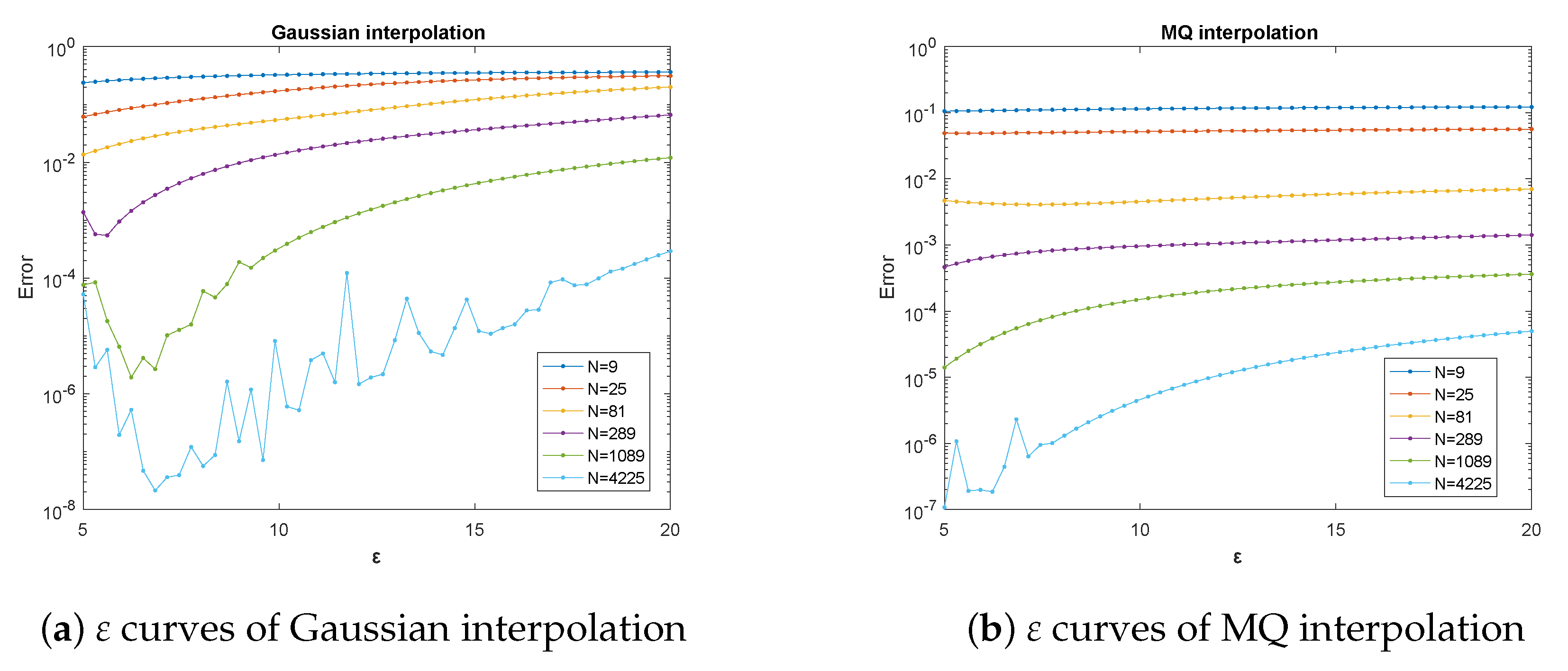
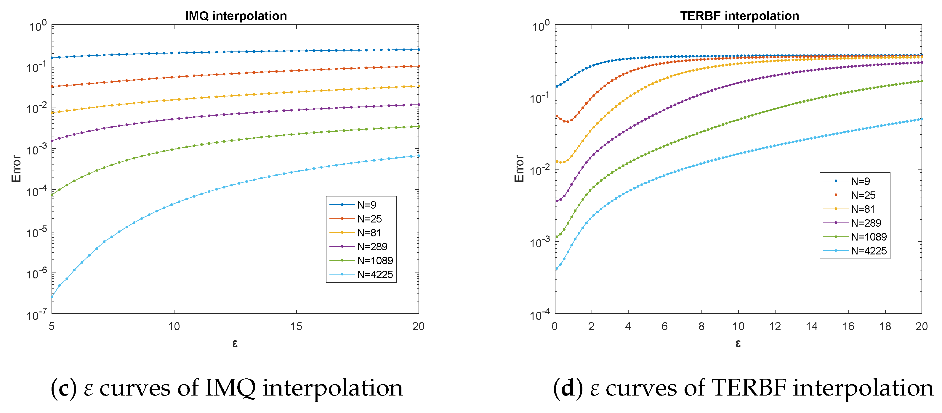
). The change of RMS-error with varying ε values is displayed in 
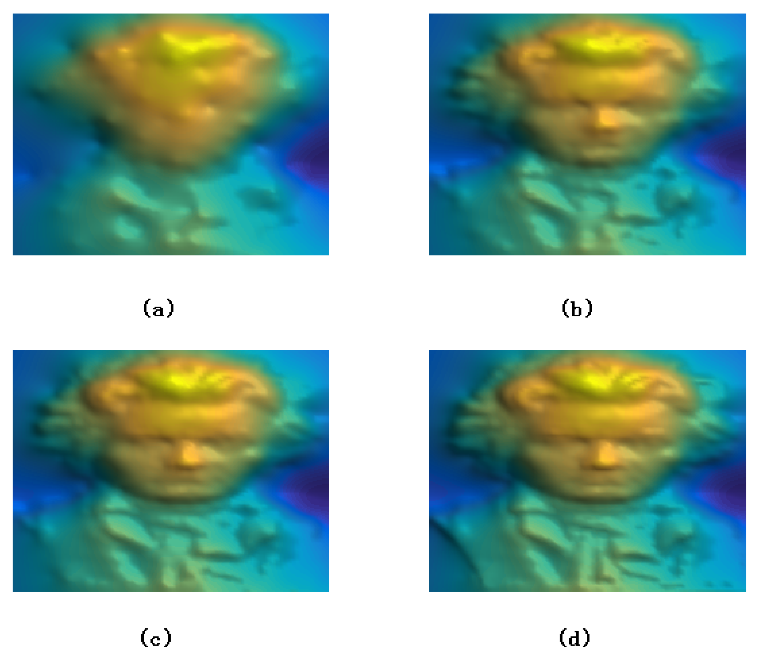
Figure 1. We see that the error curves of Gaussian and MQ interpolation are not monotonic and even become erratic for the largest datasets. However, the curves of IMQ and TERBF interpolation are relatively smooth. In particular, TERBF greatly improves the condition number of the interpolation matrix. To show the application of TERBF approximation to compact 3D images, we interpolate Beethoven data in 
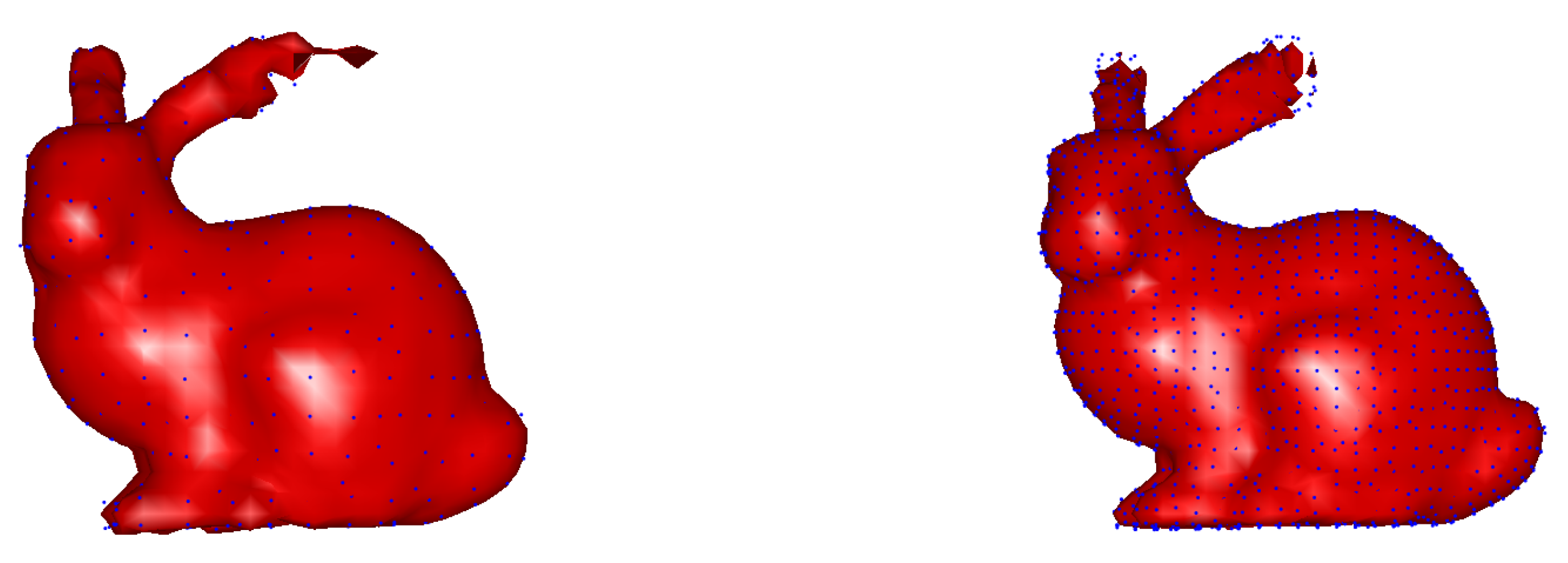
Figure 2 and Stanford bunny in Figure 3. Numerical experiments suggest that TERBF interpolation is essentially faster than the scattered data interpolation with globally supported radial basis functions. However, we observe that TERBF interpolation causes some artifacts such as the extra surface fragment near the bunny’s ear from the left part of Figure 3. This is because the interpolating implicit surface has a narrow band support. It will be better if the sample density is smaller than the width of the support band (see the right part of Figure 3). Similar observations have been reported in Fasshauer’s book [3], where a partition of unity fits based on Wendland’s C 2 function was used. The same observation was also made in [1].

5.2. Multilevel Approximation

The multilevel scattered approximation was implemented first in [8] and then studied by a number of other researchers [9,10,11,12,13]. In the multilevel algorithm, the residual can be formed on the coarsest level first and then be approximated on the later finer level by the compactly supported radial basis functions with gradually smaller support. This process can be repeated and be stopped on the finest level. An advantage of this multilevel interpolation algorithm is its recursive property (i.e., the same routine can be applied recursively at each level in the programming language), of course the disadvantage being the allocation that memory needs.
In this experiment, suppose a 3D target surface is an explicit function f ( x , y , z ) = 64 x ( 1 x ) y ( 1 y ) z ( 1 z ) . We generate a uniform points set in the domain [ 0 , 1 ] 3 , with levels k = 1 , 2 , 3 , 4 and N = 27 , 125 , 729 , 4913 . The scale parameter ε = 0.07 × 2 [ 0 : 3 ] , and l = 3 . The corresponding slice plots, the iso-surfaces, and slice plots of the absolute error are shown in Figure 4, Figure 5, Figure 6 and Figure 7. Both the iso-surfaces and the slice plots are color coded according to the absolute error. At each level, the trial space is constructed by a series of truncated exponential radial basis functions with varying support radii. Hence, the multilevel approximation algorithm can produce a well conditioned sparse discrete algebraic system in each recursion and keep ideal approximation accuracy at the same time. Numerical experiments show that TERBF multilevel interpolation is very effective for 3D explicit surface approximation. These observations can be found from Figure 4, Figure 5, Figure 6 and Figure 7. Similar experiments and observations are reported in detail in Fasshauer’s book [3], where Wendland’s function C 4 has been used for approximation. However, to improve the allocation memory needs of the multilevel algorithm, we can make use of the hierarchical collocation method developed in [13].

6. Conclusions

The truncated exponential radial function, which has compact support, was introduced in the paper. The strictly positive definiteness of TERBF was proven via the multiply monotonicity approach, and the interpolation error estimates were obtained via the native space approach. Moreover, the TERBF was applied to 2D/3D scattered data interpolation and surface modeling successfully.
However, we found that Φ ( x ) = ( e 1 ε x 1 ) + l was only in C 0 space. In the error estimates in terms of the fill distance, the power of h X , Ω was only 1 / 2 . There are many possibilities for enhancement of TERBF approximation:
(1) We can construct new strictly positive definite radial functions with finite smoothness from the given Φ ( x ) by a “dimension-walk” technique.
(2) We can do in-depth analysis of the characterization of TERBF in terms of Fourier transforms established by Bochner and Schoenberg’s theorems.
(3) TERBF can also be used for the numerical solution of partial differential equations. The convergence proof will depend on the approximation of TERBF trial spaces, the appropriate inverse inequality, and the sampling theorem.

Author Contributions

Conceptualization, Methodology and Writing–original draft preparation, Q.X.; Formal analysis and Writing—review and editing, Z.L.

Funding

The research of the first author was partially supported by the Natural Science Foundations of Ningxia Province (No. NZ2018AAC03026) and the Fourth Batch of the Ningxia Youth Talents Supporting Program (No. TJGC2019012). The research of the second author was partially supported by the Natural Science Foundations of China (No. 11501313), the Natural Science Foundations of Ningxia Province (No. 2019AAC02001), the Project funded by the China Postdoctoral Science Foundation (No. 2017M621343), and the Third Batch of the Ningxia Youth Talents Supporting Program (No. TJGC2018037).

Acknowledgments

The authors would like to thank the Editor and two unknown reviewers who made valuable comments on an earlier version of this paper. The authors used some Halton datasets and drew lessons from partial codes from Fasshauer’s book [3]. We are grateful to [3] for its free CD, which contains many MATLAB codes.

Conflicts of Interest

The authors declare no conflict of interest.

References

  1. Ohtake, Y.; Belyaev, A.; Seidel, H.P. 3D scattered data interpolation and approximation with multilevel compactly supported RBFs. Graph. Model. 2005, 67, 150–165. [Google Scholar] [CrossRef]
  2. Wendland, H. Scattered Data Approximation; Cambridge University Press: Cambridge, UK, 2005. [Google Scholar]
  3. Fasshauer, G.E. Meshfree Approximation Methods with MATLAB; World Scientific Publishers: Singapore, 2007. [Google Scholar]
  4. Micchelli, C.A. Interpolation of scattered data: Distance matrices and conditionally positive definite functions. Constr. Approx. 1986, 2, 11–22. [Google Scholar] [CrossRef]
  5. Schaback, R. A unified theory of radial basis functions: Native Hilbert spaces for radial basis functions II. J. Comp. Appl. Math. 2000, 121, 165–177. [Google Scholar] [CrossRef]
  6. De Marchi, S.; Perracchiono, E. Lectures on Radial Basis Functions; Department of Mathematics, “Tullio Levi-Civita”, University of Padova: Padova, Italy; Available online: https://www.google.com/url?sa=t&rct=j&q=&esrc=s&source=web&cd=1&ved=2ahUKEwjkuuu01ejlAhW9xosBHaZ0Ct8QFjAAegQIABAC&url=https%3A%2F%2Fwww.math.unipd.it%2F~demarchi%2FRBF%2FLectureNotes_new.pdf&usg=AOvVaw0sDK5WcNE1POWoa_lVur9v (accessed on 20 October 2019).
  7. Bernard, C.P.; Mallat, S.G.; Slotine, J.J. Scattered data interpolation with wavelet trees. In Curve and Surface Fitting (Saint-Malo, 2002); Nashboro Press: Brentwood, TN, USA, 2003; pp. 59–64. [Google Scholar]
  8. Floater, M.S.; Iske, A. Multistep scattered data interpolation using compactly supported radial basis functions. J. Comput. Appl. Math. 1996, 73, 65–78. [Google Scholar] [CrossRef]
  9. Chen, C.S.; Ganesh, M.; Golberg, M.A.; Cheng, A.H.D. Multilevel compact radial functions based computational schemes for some elliptic problems. Comput. Math. Appl. 2002, 43, 359–378. [Google Scholar] [CrossRef]
  10. Chernih, A.; Gia, Q.T.L. Multiscale methods with compactly supported radial basis functions for the Stokes problem on bounded domains. Adv. Comput. Math. 2016, 42, 1187–1208. [Google Scholar] [CrossRef]
  11. Farrell, P.; Wendland, H. RBF multiscale collocation for second order elliptic boundary value problems. SIAM J. Numer. Anal. 2013, 51, 2403–2425. [Google Scholar] [CrossRef]
  12. Fasshauer, G.E.; Jerome, J.W. Multistep approximation algorithms: Improved convergence rates through postconditioning with smoothing kernels. Adv. Comput. Math. 1999, 10, 1–27. [Google Scholar] [CrossRef]
  13. Liu, Z.; Xu, Q. A Multiscale RBF Collocation Method for the Numerical Solution of Partial Differential Equations. Mathematics 2019, 7, 964. [Google Scholar] [CrossRef] [Green Version]
Figure 1. RMS-error curves for Gaussian, MQ, IMQ, and TERBF interpolations.
Mathematics 07 01101 g001aMathematics 07 01101 g001b
Figure 2. TERBF approximation of the Beethoven data. From top left to bottom right: 163 (a), 663 (b), 1163 (c), and 2663 (d) points.
Mathematics 07 01101 g002
Figure 3. TERBF approximation of the Stanford bunny with 453 (left) and 8171 (right) data points.
Mathematics 07 01101 g003
Figure 4. Fits and errors at Level 1.
Mathematics 07 01101 g004
Figure 5. Fits and errors at Level 2.
Mathematics 07 01101 g005
Figure 6. Fits and errors at Level 3.
Mathematics 07 01101 g006
Figure 7. Fits and errors at Level 4.
Mathematics 07 01101 g007
Table 1. Gaussian interpolation to the 2D Franke’s function with ε = 20 .
NRMS-Error Ratecond(A)
93.633326 ×  10 1 -1.000028 ×  10 + 0
253.138226 ×  10 1 0.2113411.006645 ×  10 + 0
812.003929 ×  10 1 0.6471183.170400 ×  10 + 0
2896.616318 ×  10 2 1.5987313.761572 ×  10 + 1
10891.205109 ×  10 2 2.4568651.925205 ×  10 + 5
42252.908614 ×  10 4 5.3726882.687885 ×  10 + 16
Table 2. Gaussian interpolation to the 2D Franke’s function with ε = 10 .
NRMS-Error Ratecond(A)
93.256546 ×  10 1 -1.129919 ×  10 + 0
251.722746 ×  10 1 0.9186331.667637 ×  10 + 0
815.465624 ×  10 2 1.6562522.601726 ×  10 + 1
2891.391350 ×  10 2 1.9739017.316820 ×  10 + 4
10893.273510 ×  10 4 5.4095031.179104 ×  10 + 16
42251.135157 ×  10 6 8.1718031.906108 ×  10 + 20
Table 3. MQ interpolation to the 2D Franke’s function with ε = 20 .
NRMS-Error Ratecond(A)
91.224583 ×  10 1 -5.366051 ×  10 + 1
255.646454 ×  10 2 1.1168743.124063 ×  10 + 2
816.998841 ×  10 3 3.0121575.534539 ×  10 + 3
2891.418117 ×  10 3 2.3031392.324743 ×  10 + 5
10893.627073 ×  10 4 1.9670998.803829 ×  10 + 7
42254.969932 ×  10 5 2.8675085.331981 ×  10 + 11
Table 4. MQ interpolation to the 2D Franke’s function with ε = 10 .
NRMS-Error Ratecond(A)
91.146184 ×  10 1 -8.464360 ×  10 + 1
255.193997 ×  10 2 1.1419216.680998 ×  10 + 2
814.534144 ×  10 3 3.5179432.158362 ×  10 + 4
2899.608696 ×  10 4 2.2384185.033541 ×  10 + 6
10891.506154 ×  10 4 2.6734713.025049 ×  10 + 10
42254.603113 ×  10 6 5.0321165.613893 ×  10 + 16
Table 5. IMQ interpolation to the 2D Franke’s function with ε = 20 .
NRMS-Error Ratecond(A)
92.491443 ×  10 1 -2.733942 ×  10 + 0
259.914856 ×  10 2 1.3293186.933813 ×  10 + 0
813.257319 ×  10 2 1.6059075.444834 ×  10 + 1
2891.159691 ×  10 2 1.4899451.022341 ×  10 + 3
10893.420734 ×  10 3 1.7613621.850967 ×  10 + 5
42256.703871 ×  10 4 2.3512405.607685 ×  10 + 8
Table 6. IMQ interpolation to the 2D Franke’s function with ε = 10 .
NRMS-Error Ratecond(A)
92.065836 ×  10 1 -5.995564 ×  10 + 0
255.366442 ×  10 2 1.9446882.312141 ×  10 + 1
811.517723 ×  10 2 1.8220574.053520 ×  10 + 2
2895.181480 ×  10 3 1.5504723.889766 ×  10 + 4
10899.630601 ×  10 4 2.4276671.155244 ×  10 + 8
42254.615820 ×  10 5 4.3829671.158439 ×  10 + 14
Table 7. TERBF interpolation to the 2D Franke’s function with ε = 1 .
NRMS-Error Ratecond(A)
91.951235 ×  10 1 -6.639719 ×  10 + 0
255.018953 ×  10 2 1.9589292.405994 ×  10 + 1
811.628459 ×  10 2 1.6238791.669026 ×  10 + 2
2896.727682 ×  10 3 1.2753261.250365 ×  10 + 3
10892.402630 ×  10 3 1.4854951.058555 ×  10 + 4
42259.728457 ×  10 4 1.3043329.410946 ×  10 + 4
Table 8. TERBF interpolation to the 2D Franke’s function with ε = 0.7 .
NRMS-Error Ratecond(A)
91.728785 ×  10 1 -1.275042 ×  10 + 1
254.535991 ×  10 2 1.9302695.066809 ×  10 + 1
811.335521 ×  10 2 1.7640153.608813 ×  10 + 2
2895.013012 ×  10 3 1.4136532.719227 ×  10 + 3
10891.773595 ×  10 3 1.4990012.305630 ×  10 + 4
42257.107796 ×  10 4 1.3192032.050036 ×  10 + 5

