Article

Convergence Analysis and Complex Geometry of an Efficient Derivative-Free Iterative Method

by
Deepak Kumar
1,2,*,†,
Janak Raj Sharma
1,*,† and
Lorentz Jäntschi
3,4,*
1
Department of Mathematics, Sant Longowal Institute of Engineering and Technology, Longowal 148106, Sangrur, India
2
Chandigarh University, Gharuan 140413, Mohali, India
3
Department of Physics and Chemistry, Technical University of Cluj-Napoca, Cluj-Napoca 400114, Romania
4
Institute of Doctoral Studies, Babeş-Bolyai University, Cluj-Napoca 400084, Romania
*
Authors to whom correspondence should be addressed.
These authors contributed equally to this work.
Mathematics 2019, 7(10), 919; https://doi.org/10.3390/math7100919
Submission received: 12 September 2019 / Revised: 27 September 2019 / Accepted: 29 September 2019 / Published: 2 October 2019
(This article belongs to the Special Issue Numerical Methods)

Abstract

:
To locate a locally-unique solution of a nonlinear equation, the local convergence analysis of a derivative-free fifth order method is studied in Banach space. This approach provides radius of convergence and error bounds under the hypotheses based on the first Fréchet-derivative only. Such estimates are not introduced in the earlier procedures employing Taylor’s expansion of higher derivatives that may not exist or may be expensive to compute. The convergence domain of the method is also shown by a visual approach, namely basins of attraction. Theoretical results are endorsed via numerical experiments that show the cases where earlier results cannot be applicable.

1. Introduction

Banach [1] or complete normed vector spaces constantly bring new solving strategies for real problems in domains dealing with numerical methods (see for example [2,3,4,5]). In this context, development of new methods [6] and their convergence analysis [7] are of growing interest.
Let B 1 , B 2 be Banach spaces and Ω B 1 be closed and convex. In this study, we locate a solution x of the nonlinear equation
F ( x ) = 0 ,
where F : Ω B 1 B 2 is a Fréchet-differentiable operator. In computational sciences, many problems can be transformed into form (1). For example, see the References [8,9,10,11]. The solution of such nonlinear equations is hardly attainable in closed form. Therefore, most of the methods for solving such equations are usually iterative. The important issue addressed to an iterative method is its domain of convergence since it gives us the degree of difficulty for obtaining initial points. This domain is generally small. Thus, it is necessary to enlarge the domain of convergence but without any additional hypotheses. Another important problem related to convergence analysis of an iterative method is to find precise error estimates on x n + 1 x n or x n x .
A good reference for the general principles of functional analysis is [12]. Recurrence relations for rational cubic methods are revised in [13] (for Halley method) and in [14] (for Chebyshev method). A new iterative modification of Newton’s method for solving nonlinear scalar equations was proposed in [15], while a modification of a variant of it with accelerated third order convergence was proposed in [16]. An ample collection of iterative methods is found in [9]. The recurrence relations for Chebyshev-type methods accelerating classical Newton iteration have been introduced in [17], recurrence relations in a third-order family of Newton-like methods for approximating solution of a nonlinear equation in Banach spaces were studied in [18]. In the context of Kantrovich assumptions for semilocal convergence of a Chebyshev method, the convergence conditions are significantly reduced in [19]. The computational efficiency and the domain of the uniqueness of the solution were readdressed in [20]. The point of attraction of two fourth-order iterative Newton-type methods was studied in [21], while convergence ball and error analysis of Newton-type methods with cubic convergence were studied in [22,23]. Weaker conditions for the convergence of Newton’s method are given in [24], while further analytical improvements in two particular cases as well as numerical analysis in the general case are given in [25], while local convergence of three-step Newton–Gauss methods in Banach spaces was recently analyzed in [26]. Recently, researchers have also constructed some higher order methods; see, for example [27,28,29,30,31] and references cited therein.
One of the basic methods for approximating a simple solution x of Equation (1) is the quadratically convergent derivative-free Traub–Steffensen’s method, which is given by
x n + 1 = M 2 , 1 ( x n ) = x n [ u n , x n ; F ] 1 F ( x n ) , for each n = 0 , 1 , 2 , ,
where u n = x n + β F ( x n ) , β R { 0 } has a quadratic order of convergence. Based on (2), Sharma et al. [32] have recently proposed a derivative-free method with fifth order convergence for approximating a solution of F ( x ) = 0 using the weight-function scheme defined for each n = 0 , 1 by
y n = M 2 , 1 ( x n ) , z n = y n [ u n , x n ; F ] 1 F ( y n ) , x n + 1 = z n H ( x n ) [ u n , x n ; F ] 1 F ( z n ) ,
wherein H ( x n ) = 2 I [ u n , x n ; F ] 1 [ z n , y n ; F ] . The computational efficiency of this method was discussed in detail and performance was favorably compared with existing methods in [32]. To prove the local convergence order, the authors used Taylor expansions with hypotheses based on a Fréchet-derivative up to the fifth order. It is quite clear that these hypotheses restrict the applicability of methods to the problems involving functions that are at least five times Fréchet-differentiable. For example, let us define a function g on Ω = [ 1 2 , 5 2 ] by
g ( t ) = t 3 ln t 2 + t 5 t 4 , t 0 , 0 , t = 0 .
We have that
g ( t ) = 3 t 2 ln t 2 + 5 t 4 4 t 3 + 2 t 2 ,
g ( t ) = 6 t ln t 2 + 20 t 3 12 t 2 + 10 t
and
g ( t ) = 6 ln t 2 + 60 t 2 24 t + 22 .
Then, g is unbounded on Ω . Notice also that the proofs of convergence use Taylor expansions.
In this work, we study the local convergence of the methods (3) using the hypotheses on the first Fréchet-derivative only taking advantage of the Lipschitz continuity of the first Fréchet-derivative. Moreover, our results are presented in the more general setting of a Banach space. We summarize the contents of the paper. In Section 2, the local convergence analysis of method (3) is presented. In Section 3, numerical examples are performed to verify the theoretical results. Basins of attraction showing convergence domain are drawn in Section 4. Concluding remarks are reported in Section 5.

2. Local Convergence Analysis

Let’s study the local convergence of method (3). Let p 0 and M 0 be the parameters and w 0 : [ 0 , + ) 2 [ 0 , + ) be a continuous and nondecreasing function with w 0 ( 0 , 0 ) = 0 . Let the parameter r be defined by
r = sup { t 0 ; w 0 ( p t , t ) < 1 } .
Consider the functions w 1 : [ 0 , r ) 2 [ 0 , + ) and v 0 : [ 0 , r ) [ 0 , + ) as continuous and nondecreasing. Furthermore, define functions g 1 and h 1 on the interval [ 0 , r ) as
g 1 ( t ) = w 1 ( β v 0 ( t ) t , t ) 1 w 0 ( p t , t )
and
h 1 ( t ) = g 1 ( t ) 1 .
Suppose that
w 1 ( 0 , 0 ) < 1 .
From (6), we obtain that
h 1 ( 0 ) = w 1 ( 0 , 0 ) 1 w 0 ( 0 , 0 ) 1 < 0
and, by (5), h 1 ( t ) + as t r . Then, it follows from the intermediate value theorem [33] that equation h 1 ( t ) = 0 has solutions in ( 0 , r ) . Denote by r 1 the smallest such solution.
Furthermore, define functions g 2 and h 2 on the interval [ 0 , r 1 ) by
g 2 ( t ) = 1 + M 1 w 0 ( p t , t ) g 1 ( t )
and
h 2 ( t ) = g 2 ( t ) 1 .
Then, we have that h 2 ( 0 ) = 1 < 0 and h 2 ( t ) + as t r 1 . Let r 2 be the smallest zero of function h 2 on the interval ( 0 , r 1 ) .
Finally, define the functions g ¯ , g 3 and h 3 on the interval [ 0 , r 2 ) by
g ¯ ( t ) = 1 1 w 0 ( p t , t ) 1 + w 0 ( p t , t ) + w 0 ( g 1 ( t ) t , g 2 t ) 1 w 0 ( p t , t ) ,
g 3 ( t ) = 1 + M g ¯ ( t ) g 2 ( t )
and
h 3 ( t ) = g 3 ( t ) 1 .
It follows that h 3 ( t ) = 1 < 0 and h 3 ( t ) + as t r 2 . Denote the smallest zero of function h 3 by r 3 on the interval ( 0 , r 2 ) . Finally, define the radius of convergence (say, r ) by
r = min { r i } , i = 1 , 2 , 3 .
Then, for each t [ 0 , r ) , we have that
0 g i ( t ) < 1 , i = 1 , 2 , 3 .
Denote by U ( ν , ε ) = { x B 1 : x ν < ε } the ball whose center ν B 1 and radius ε > 0 . Moreover, U ¯ ( ν , ε ) denotes the closure of U ( ν , ε ) .
We will study the local convergence of method (3) in a Banach space setting under the following hypotheses (collectively called by the name ‘A’):
(a1)
F : Ω B 1 B 2 is a continuously differentiable operator and [ · , · ; F ] : Ω × Ω L ( B 1 , B 2 ) is a first divided difference operator of F.
(a2)
There exists x Ω so that F ( x ) = 0 and F ( x ) 1 L ( B 2 , B 1 ) .
(a3)
There exists a continuous and nondecreasing function w 0 : R + { 0 } R + { 0 } with w 0 ( 0 ) = 0 such that, for each x Ω ,
F ( x ) 1 ( [ x , y ; F ] F ( x ) ) w 0 ( x x , y x ) .
(a4)
Let Ω 0 = Ω U ( x , r ) , where r has been defined before. There exists continuous and nondecreasing function v 0 : [ 0 , r ) R + { 0 } such that, for each x , y Ω 0 ,
β [ x , x ; F ] v 0 ( x 0 x ) ,
U ¯ ( x , r ) Ω ,
I + β [ x , x ; F ] p .
(a5)
U ¯ ( x , r 3 ) Ω and F ( x ) 1 F ( x ) M .
(a6)
Let R r 3 and set Ω 1 = Ω U ¯ ( x , R ) , 0 1 w 0 ( θ R ) d θ < 1 .
Theorem 1.
Suppose that the hypotheses ( A ) hold. Then, the sequence { x n } generated by method (3) for x 0 U ( x , r 3 ) { x } is well defined in U ( x , r 3 ) , remains in U ( x , r 3 ) and converges to x . Moreover, the following conditions hold:
y n x g 1 ( x n x ) x n x x n x < ϱ ,
z n x g 2 ( x n x ) x n x x n x
and
x n + 1 x g 3 ( x n x ) x n x x n x ,
where the functions g i , i = 1 , 2 , 3 are defined as above. Furthermore, the vector x is the only solution of F ( x ) = 0 in Ω 1 .
Proof. 
We shall show estimates (9)–(11) using mathematical induction. By hypothesis (a3) and for x U ( x , r 3 ) , we have that
F ( x ) 1 ( [ u 0 , x 0 ; F ] F ( x ) ) w 0 ( u 0 x , x 0 x ) w 0 ( x 0 x + β F ( x 0 ) , x 0 x ) w 0 ( ( I + β [ x 0 , x ; F ] ) x 0 x , x 0 x ) w 0 ( p x 0 x , x 0 x ) w 0 ( p r , r ) < 1 .
By (12) and the Banach Lemma [9], we have that [ u n , x n ; F ] 1 L ( B 2 , B 1 ) and
[ u 0 , x 0 ; F ] 1 F ( x ) 1 1 w 0 ( p x 0 x , x 0 x ) .
We show that y n is well defined by the method (3) for n = 0 . We have
y 0 x = x 0 x [ u 0 , x 0 ; F ] 1 F ( x 0 ) = [ u 0 , x 0 ; F ] 1 F ( x ) F ( x ) 1 [ u 0 , x 0 ; F ] [ x 0 , x ; F ] ( x 0 x ) .
Then, using (8) (for i = 1 ), the conditions (a4) and (13), we have in turn that
y 0 x = [ u 0 , x 0 ; F ] 1 F ( x ) F ( x ) 1 [ u 0 , x 0 ; F ] [ x n , x ; F ] x 0 x w 1 ( u 0 x 0 , x 0 x ) x 0 x 1 w 0 ( p x 0 x , x 0 x ) w 1 ( β F ( x 0 ) , x 0 x ) x 0 x 1 w 0 ( p x 0 x , x 0 x ) w 1 ( β [ x 0 , x ; F ] ( x 0 x ) , x 0 x ) 1 w 0 ( p x 0 x , x 0 x ) x 0 x w 1 ( β v 0 ( x 0 x ) ( x 0 x ) , x 0 x ) 1 w 0 ( p x 0 x , x 0 x ) x 0 x g 1 ( x 0 x ) x 0 x < x 0 x < r ,
which implies (9) for n = 0 and y 0 U ( x , r 3 ) .
Note that for each θ [ 0 , 1 ] and x + θ ( x 0 x ) x = θ x 0 x < r , that is, x + θ ( x 0 x ) U ( x , r 3 ) , writing
F ( x 0 ) = F ( x 0 ) F ( x ) = 0 1 F ( x + θ ( x 0 x ) ) ( x 0 x ) d θ .
Then, using (a5), we get that
F ( x ) 1 F ( x 0 ) = 0 1 F ( x ) 1 F ( x + θ ( x 0 x ) ) ( x 0 x ) d θ M x 0 x .
Similarly, we obtain
F ( x ) 1 F ( y 0 ) M y 0 x ,
F ( x ) 1 F ( z 0 ) M z 0 x .
From the second sub-step of method (3), (13), (15) and (18), we obtain that
z 0 x y 0 x + [ u 0 , x 0 ; F ] 1 F ( x ) F ( x ) 1 F ( y 0 ) y 0 x + M y 0 x 1 w 0 ( p x 0 x , x 0 x ) 1 + M 1 w 0 ( p x 0 x , x 0 x ) y 0 x 1 + M 1 w 0 ( p x 0 x , x 0 x ) g 1 ( x 0 x ) x 0 x g 2 ( x 0 x ) x 0 x < x 0 x < r ,
which proves (10) for n = 0 and z 0 U ( x , r 3 ) .
Let ψ ( x n , y n ) = 2 I [ u n , x n ; F ] 1 [ y n , z n ; F ] [ u n , x n ; F ] 1 and notice that, since x 0 , y 0 U ( x , r 3 ) , we have that
ψ ( x 0 , y 0 ) F ( x ) = 2 I [ u 0 , x 0 ; F ] 1 [ y 0 , z 0 ; F ] [ u 0 , x 0 ; F ] 1 F ( x ) 1 + [ u 0 , x 0 ; F ] 1 [ u 0 , x 0 ; F ] [ y 0 , z 0 ; F ] [ u 0 , x 0 ; F ] 1 F ( x ) ( 1 + [ u 0 , x 0 ; F ] 1 F ( x ) ( F ( x ) 1 ( [ u 0 , x 0 ; F ] F ( x ) ) + F ( x ) 1 ( F ( x ) [ y 0 , z 0 ; F ] ) ) ) [ u 0 , x 0 ; F ] 1 F ( x ) 1 + w 0 ( p x n x , x n x ) + w 0 y 0 x , z 0 x 1 w 0 ( p x n x , x n x ) × 1 1 w 0 ( p x n x , x n x ) 1 + w 0 ( p x n x , x n x ) + w 0 g 1 ( x 0 x ) x 0 x , g 2 ( x 0 x ) x 0 x 1 w 0 ( p x n x , x n x ) × 1 1 w 0 ( p x n x , x n x ) g ¯ ( x 0 x ) .
Then, using Equation (8) (for i = 3 ), (19), (20) and (21), we obtain
x 1 x = z 0 x ψ ( x 0 , y 0 ) F ( z 0 ) z 0 x + ψ ( x 0 , y 0 ) F ( x ) F ( x ) 1 F ( z 0 ) z 0 x + g ¯ ( x 0 x ) M z 0 x = 1 + M g ¯ ( x 0 x ) z 0 x 1 + M g ¯ ( x 0 x ) g 2 ( x 0 x ) x 0 x g 3 ( x 0 x ) x 0 x ,
which proves (11) for n = 0 and x 1 U ( x , r 3 ) .
Replace x 0 , y 0 , z 0 , x 1 by x n , y n , z n , x n + 1 in the preceding estimates to obtain (9)–(11). Then, from the estimates x n + 1 x c x n x < r 3 , where c = g 3 ( x 0 x ) [ 0 , 1 ) , we deduce that lim n x n = x and x n + 1 U ( x , r 3 ) .
Next, we show the uniqueness part using conditions (a3) and (a6). Define operator P by P = 0 1 F ( x + θ ( x x ) ) d θ for some x Ω 1 with F ( x ) = 0 . Then, we have that
F ( x ) 1 P F ( x ) 0 1 w 0 ( θ x x ) d θ 0 1 w 0 ( θ ϱ ) d θ < 1 ,
so P 1 L ( B 2 , B 1 ) . Then, from the identity
0 = F ( x ) F ( x ) = P ( x x ) ,
it implies that x = x . ☐

3. Numerical Examples

We illustrate the theoretical results shown in Theorem 1. For the computation of divided difference, let us choose [ x , y ; F ] = 0 1 F ( y + θ ( x y ) ) d θ . Consider the following three numerical examples:
Example 1.
Assume that the motion of a particle in three dimensions is governed by a system of differential equations:
f 1 ( x ) f 1 ( x ) 1 = 0 , f 2 ( y ) ( e 1 ) y 1 = 0 , f 3 ( z ) 1 = 0 ,
with x , y , z Ω for f 1 ( 0 ) = f 2 ( 0 ) = f 3 ( 0 ) = 0 . A solution of the system is given for u = ( x , y , z ) T by function F : = ( f 1 , f 2 , f 3 ) : Ω R 3 defined by
F ( u ) = e x 1 , e 1 2 y 2 + y , z T .
Its Fréchet-derivative F ( u ) is given by
F ( u ) = e x 0 0 0 ( e 1 ) y + 1 0 0 0 1 .
Then, for x = ( 0 , 0 , 0 ) T , we deduce that w 0 ( s , t ) = w 1 ( s , t ) = L 0 2 ( s + t ) and v 0 ( t ) = 1 2 ( 1 + e 1 L 0 ) , p = 1 + 1 2 ( 1 + e 1 L 0 ) , β = 1 100 , where L 0 = e 1 and M = 2 . Then, using a definition of parameters, the calculated values are displayed as
r = min { r 1 , r 2 , r 3 } = min { 0 . 313084 , 0 . 165881 , 0 . 0715631 } = 0 . 0715631 .
Example 2.
Let X = C [ 0 , 1 ] , Ω = U ¯ ( x , 1 ) . We consider the integral equation of the mixed Hammerstein-type [9] given by
x ( s ) = 0 1 k ( s , t ) x ( t ) 2 2 d t ,
wherein the kernel k is the green function on the interval [ 0 , 1 ] × [ 0 , 1 ] defined by
k ( s , t ) = ( 1 s ) t , t s , s ( 1 t ) , s t .
Solution x ( s ) = 0 is the same as the solution of equation F ( x ) = 0 , where F : C [ 0 , 1 ] is given by
F ( x ) ( s ) = x ( s ) 0 1 k ( s , t ) x ( t ) 2 2 d t .
Observe that
0 1 k ( s , t ) d t 1 8 .
Then, we have that
F ( x ) y ( s ) = y ( s ) 0 1 k ( s , t ) x ( t ) d t ,
and F ( x ( s ) ) = I . We can choose w 0 ( s , t ) = w 1 ( s , t ) = s + t 16 , v 0 ( t ) = 9 16 , p = 25 16 , β = 1 100 and M = 2 . Then, using a definition of parameters, the calculated values are displayed as
r = min { r 1 , r 2 , r 3 } = min { 4 . 4841 , 2 . 3541 , 1 . 0090 } = 1 . 0090 .
Example 3.
Let B 1 = B 2 = C [ 0 , 1 ] be the spaces of continuous functions defined on the interval [ 0 , 1 ] . Define function F on Ω = U ¯ ( 0 , 1 ) by
F ( φ ) ( x ) = ϕ ( x ) 10 0 1 x θ φ ( θ ) 3 d θ .
It follows that
F ( φ ( ξ ) ) ( x ) = ξ ( x ) 30 0 1 x θ φ ( θ ) 2 ξ ( θ ) d θ , f o r e a c h ξ Ω .
Then, for x = 0 , we have that w 0 ( s , t ) = w 1 ( s , t ) = L 0 ( s + t ) and v 0 ( t ) = 2 , p = 3 , β = 1 100 , where L 0 = 15 and M = 2 . The parameters are displayed as
r = min { r 1 , r 2 , r 3 } = min { 0 . 013280 , 0 . 0076012 , 0 . 0034654 } = 0 . 0034654 .

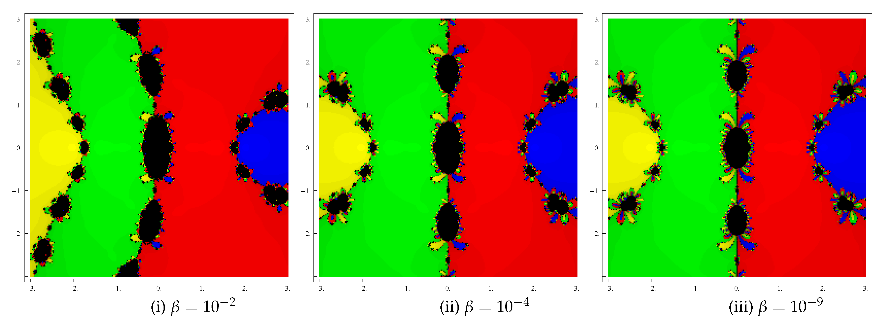
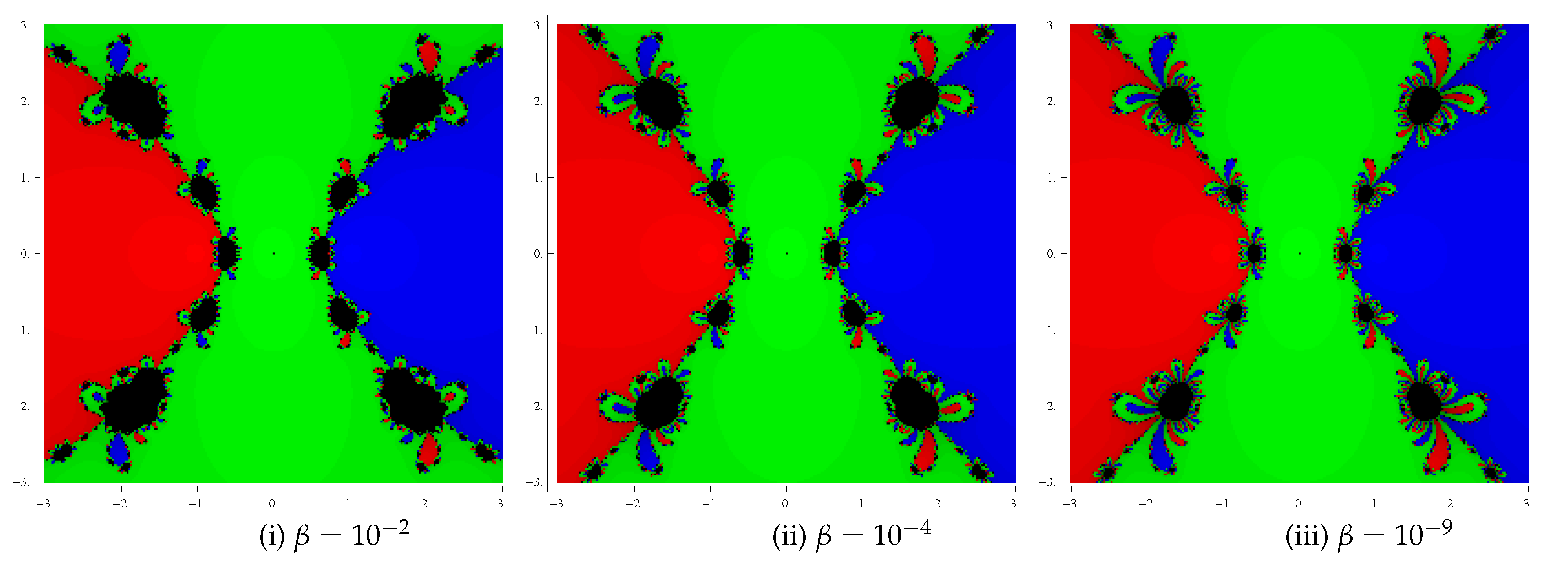
4. Basins of Attraction

The basin of attraction is a useful geometrical tool for assessing convergence regions of the iterative methods. These basins show us all the starting points that converge to any root when we apply an iterative method, so we can see in a visual way which points are good choices as starting points and which are not. We take the initial point as z 0 R , where R is a rectangular region in C containing all the roots of a poynomial p ( z ) = 0 . The iterative methods starting at a point z 0 in a rectangle can converge to the zero of the function p ( z ) or eventually diverge. In order to analyze the basins, we consider the stopping criterion for convergence as 10 3 up to a maximum of 25 iterations. If the mentioned tolerance is not attained in 25 iterations, the process is stopped with the conclusion that the iterative method starting at z 0 does not converge to any root. The following strategy is taken into account: A color is assigned to each starting point z 0 in the basin of attraction of a zero. If the iteration starting from the initial point z 0 converges, then it represents the basins of attraction with that particular color assigned to it and, if it fails to converge in 25 iterations, then it shows the black color.
We analyze the basins of attraction on the following two problems:
Test problem 1. Consider the polynomial p 1 ( z ) = z 4 6 z 2 + 8 that has four simple zeros { ± 2 , ± 1 . 414 } . We use a grid of 400 × 400 points in a rectangle R C of size [ 3 , 3 ] × [ 3 , 3 ] and allocate the red, blue, green and yellow colors to the basins of attraction of these four zeros. Basins obtained for the method (3) are shown in Figure 1(i)–(iii) corresponding to β = 10 2 , 10 4 , 10 9 . Observing the behavior of the method, we say that the divergent zones (black zones) are becoming smaller with the decreasing value of β .
Problem 2. Let us take the polynomial p 2 ( z ) = z 3 z having zeros { 0 , ± 1 } . In this case, we also consider a rectangle R = [ 3 , 3 ] × [ 3 , 3 ] C with 400 × 400 grid points and allocate the colors red, green and blue to each point in the basin of attraction of 1 , 0 and 1, respectively. Basins obtained for the method (3) are displayed in Figure 2(i)–(iii) for the parameter values β = 10 2 , 10 4 , 10 9 . Notice that the divergent zones are becoming smaller in size as parameter β assumes smaller values.

5. Conclusions

In this paper, the local convergence analysis of a derivative-free fifth order method is studied in Banach space. Unlike other techniques that rely on higher derivatives and Taylor series, we have used only derivative of order one in our approach. In this way, we have extended the usage of the considered method since the method can be applied to a wider class of functions. Another advantage of analyzing the local convergence is the computation of a convergence ball, uniqueness of the ball where the iterates lie and estimation of errors. Theoretical results of convergence thus achieved are confirmed through testing on some practical problems.
The basins of attraction have been analyzed by applying the method on some polynomials. From these graphics, one can easily visualize the behavior and suitability of any method. If we choose an initial guess x 0 in a domain where different basins of the roots meet each other, it is uncertain to predict which root is going to be reached by the iterative method that begins from x 0 . Thus, the choice of initial guess lying in such a domain is not suitable. In addition, black zones and the zones with different colors are not suitable to take the initial guess x 0 when we want to achieve a particular root. The most attractive pictures appear when we have very intricate boundaries of the basins. Such pictures belong to the cases where the method is more demanding with respect to the initial point.

Author Contributions

Methodology, D.K.; writing, review and editing, J.R.S.; investigation, J.R.S.; data curation, D.K.; conceptualization, L.J.; formal analysis, L.J.

Funding

This research received no external funding.

Acknowledgments

We would like to express our gratitude to the anonymous reviewers for their valuable comments and suggestions which have greatly improved the presentation of this paper.

Conflicts of Interest

The authors declare no conflict of interest.

References

  1. Banach, S. Théorie des Opérations Linéare; Monografje Matematyczne: Warszawna, Poland, 1932. [Google Scholar]
  2. Gupta, V.; Bora, S.N.; Nieto, J.J. Dhage iterative principle for quadratic perturbation of fractional boundary value problems with finite delay. Math. Methods Appl. Sci. 2019, 42, 4244–4255. [Google Scholar] [CrossRef]
  3. Jäntschi, L.; Bálint, D.; Bolboacă, S. Multiple linear regressions by maximizing the likelihood under assumption of generalized Gauss-Laplace distribution of the error. Comput. Math. Methods Med. 2016, 2016, 8578156. [Google Scholar] [CrossRef] [PubMed]
  4. Kitkuan, D.; Kumam, P.; Padcharoen, A.; Kumam, W.; Thounthong, P. Algorithms for zeros of two accretive operators for solving convex minimization problems and its application to image restoration problems. J. Comput. Appl. Math. 2019, 354, 471–495. [Google Scholar] [CrossRef]
  5. Sachs, M.; Leimkuhler, B.; Danos, V. Langevin dynamics with variable coefficients and nonconservative forces: From stationary states to numerical methods. Entropy 2017, 19, 647. [Google Scholar] [CrossRef]
  6. Behl, R.; Cordero, A.; Torregrosa, J.R.; Alshomrani, A.S. New iterative methods for solving nonlinear problems with one and several unknowns. Mathematics 2018, 6, 296. [Google Scholar] [CrossRef]
  7. Argyros, I.K.; George, S. Unified semi-local convergence for k-step iterative methods with flexible and frozen linear operator. Mathematics 2018, 6, 233. [Google Scholar] [CrossRef]
  8. Argyros, I.K.; Hilout, S. Computational Methods in Nonlinear Analysis; World Scientific Publishing Company: Hackensack, NJ, USA, 2013. [Google Scholar]
  9. Argyros, I.K. Computational Theory of Iterative Methods, Series: Studies in Computational Mathematics 15; Chui, C.K., Wuytack, L., Eds.; Elsevier: New York, NY, USA, 2007. [Google Scholar]
  10. Traub, J.F. Iterative Methods for the Solution of Equations; Prentice-Hall: Englewood Cliffs, NJ, USA, 1964. [Google Scholar]
  11. Potra, F.A.; Ptak, V. Nondiscrete Induction and Iterative Process; Research Notes in Mathematics; Pitman: Boston, MA, USA, 1984. [Google Scholar]
  12. Kantrovich, L.V.; Akilov, G.P. Functional Analysis; Pergamon Press: Oxford, UK, 1982. [Google Scholar]
  13. Candela, V.; Marquina, A. Recurrence relations for rational cubic methods I: The Halley method. Computing 1990, 44, 169–184. [Google Scholar] [CrossRef]
  14. Candela, V.; Marquina, A. Recurrence relations for rational cubic methods II: The Chebyshev method. Computing 1990, 45, 355–367. [Google Scholar] [CrossRef]
  15. Hasanov, V.I.; Ivanov, I.G.; Nebzhibov, G. A new modification of Newton’s method. Appl. Math. Eng. 2002, 27, 278–286. [Google Scholar]
  16. Kou, J.S.; Li, Y.T.; Wang, X.H. A modification of Newton’s method with third-order convergence. Appl. Math. Comput. 2006, 181, 1106–1111. [Google Scholar] [CrossRef]
  17. Ezquerro, J.A.; Hernández, M.A. Recurrence relation for Chebyshev-type methods. Appl. Math. Optim. 2000, 41, 227–236. [Google Scholar] [CrossRef]
  18. Chun, C.; Stănică, P.; Neta, B. Third-order family of methods in Banach spaces. Comput. Math. Appl. 2011, 61, 1665–1675. [Google Scholar] [CrossRef] [Green Version]
  19. Hernández, M.A.; Salanova, M.A. Modification of the Kantorovich assumptions for semilocal convergence of the Chebyshev method. J. Comput. Appl. Math. 2000, 126, 131–143. [Google Scholar] [CrossRef] [Green Version]
  20. Amat, S.; Hernández, M.A.; Romero, N. Semilocal convergence of a sixth order iterative method for quadratic equations. Appl. Numer. Math. 2012, 62, 833–841. [Google Scholar] [CrossRef]
  21. Babajee, D.K.R.; Dauhoo, M.Z.; Darvishi, M.T.; Barati, A. A note on the local convergence of iterative methods based on Adomian decomposition method and 3-node quadrature rule. Appl. Math. Comput. 2008, 200, 452–458. [Google Scholar] [CrossRef]
  22. Ren, H.; Wu, Q. Convergence ball and error analysis of a family of iterative methods with cubic convergence. Appl. Math. Comput. 2009, 209, 369–378. [Google Scholar] [CrossRef]
  23. Ren, H.; Argyros, I.K. Improved local analysis for certain class of iterative methods with cubic convergence. Numer. Algor 2012, 59, 505–521. [Google Scholar] [CrossRef]
  24. Argyros, I.K.; Hilout, S. Weaker conditions for the convergence of Newton’s method. J. Complexity 2012, 28, 364–387. [Google Scholar] [CrossRef]
  25. Gutiérrez, J.M.; Magreñán, A.A.; Romero, N. On the semilocal convergence of Newton–Kantorovich method under center-Lipschitz conditions. Appl. Math. Comput. 2013, 221, 79–88. [Google Scholar] [CrossRef]
  26. Argyros, I.K.; Sharma, J.R.; Kumar, D. Local convergence of Newton–Gauss methods in Banach space. SeMA 2016, 74, 429–439. [Google Scholar] [CrossRef]
  27. Behl, R.; Salimi, M.; Ferrara, M.; Sharifi, S.; Alharbi, S.K. Some real-life applications of a newly constructed derivative free iterative scheme. Symmetry 2019, 11, 239. [Google Scholar] [CrossRef]
  28. Salimi, M.; Nik Long, N.M.A.; Sharifi, S.; Pansera, B.A. A multi-point iterative method for solving nonlinear equations with optimal order of convergence. Jpn. J. Ind. Appl. Math. 2018, 35, 497–509. [Google Scholar] [CrossRef]
  29. Sharma, J.R.; Kumar, D. A fast and efficient composite Newton-Chebyshev method for systems of nonlinear equations. J. Complexity 2018, 49, 56–73. [Google Scholar] [CrossRef]
  30. Sharma, J.R.; Arora, H. On efficient weighted-Newton methods for solving systems of nonlinear equations. Appl. Math. Comput. 2013, 222, 497–506. [Google Scholar] [CrossRef]
  31. Lofti, T.; Sharifi, S.; Salimi, M.; Siegmund, S. A new class of three-point methods with optimal convergence order eight and its dynamics. Numer. Algor. 2015, 68, 261–288. [Google Scholar] [CrossRef]
  32. Sharma, J.R.; Kumar, D.; Jäntschi, L. On a reduced cost higher order Traub–Steffensen-like method for nonlinear systems. Symmetry 2019, 11, 891. [Google Scholar] [CrossRef]
  33. Grabnier, J.V. Who gave you the epsilon? Cauchy and the origins of rigorous calculus. Am. Math. Mon. 1983, 90, 185–194. [Google Scholar] [CrossRef]
Figure 1. Basins of attraction of method for polynomial p 1 ( z ) .
Mathematics 07 00919 g001
Figure 2. Basins of attraction of method for polynomial p 2 ( z ) .
Mathematics 07 00919 g002

