Article

Numerical Solution of the Cauchy-Type Singular Integral Equation with a Highly Oscillatory Kernel Function

1
School of Mathematics and Statistics, Central South University, Changsha 410083, China
2
School of Statistics and Mathematics, Nanjing Audit University, Nanjing 211815, China
*
Author to whom correspondence should be addressed.
Current address: School of Mathematics and Statistics, Central South University, Changsha 410083, China.
Mathematics 2019, 7(10), 872; https://doi.org/10.3390/math7100872
Submission received: 16 August 2019 / Revised: 17 September 2019 / Accepted: 18 September 2019 / Published: 20 September 2019
(This article belongs to the Special Issue Numerical Methods)

Abstract

:
This paper aims to present a Clenshaw–Curtis–Filon quadrature to approximate the solution of various cases of Cauchy-type singular integral equations (CSIEs) of the second kind with a highly oscillatory kernel function. We adduce that the zero case oscillation ( k = 0 ) proposed method gives more accurate results than the scheme introduced in Dezhbord et al. (2016) and Eshkuvatov et al. (2009) for small values of N. Finally, this paper illustrates some error analyses and numerical results for CSIEs.

1. Introduction

Integral equations have broad roots in branches of science and engineering [1,2,3,4,5,6]. Cauchy-type singular integral equations (CSIEs) of the second kind occur in electromagnetic scattering and quantum mechanics [7] and are defined as:
a u ( x ) + b π 1 1 u ( y ) K ( x , y ) y x d y = f ( x ) , x ( 1 , 1 ) .
A singular integral equation with a Cauchy principal value is a generalized form of an airfoil equation [8]. Here a and b are constants such that a 2 + b 2 = 1 , b 0 and K ( x , y ) = e i k ( y x ) are the highly oscillatory kernel function. The function f ( x ) is the Hölder continuous function, whereas u ( x ) is an unknown function. The solution to the above-mentioned Equation (1) contains boundary singularities w ( x ) = ( x + 1 ) α ( 1 x ) β , i.e., u ( x ) = w ( x ) g ( x ) and g ( x ) is a smooth function [9,10]. Then the above Equation (1) transforms into:
a w ( x ) g ( x ) + b π 1 1 w ( y ) g ( y ) e i k ( y x ) y x d y = f ( x ) , x ( 1 , 1 ) ,
where α , β ( 1 , 1 ) depend on a and b, such that:
α = 1 2 π i log a i b a + i b N , β = 1 2 π i log a i b a + i b M ,
κ = ( α + β ) = M + N .
Here M and N are integers in [ 1 , 1 ] , whereas the index of the integral equation is called κ , analogous to a class of functions, wherein the solution is to be sought. It is pertinent to mention that to produce integrable singularities in the solution, the index κ is restricted to three cases, [ 1 , 0 , 1 ] , but the addressed paper considers only two cases for κ , i.e., κ 0 . The value of the index κ depends on different values for M and N[11,12,13]. A great number of real life practical problems, e.g., for κ = 1 , the so-called natched half-plane problem and another problem of a crack parallel to the free boundary of an isotropic semi-infinite plane, that can be reduced to Cauchy singular integral equations are addressed in [14,15,16,17]. Writing Equation (2) in operator form, we get [18]:
H g = f ,
where:
H g = a w ( x ) g ( x ) + b π 1 1 w ( y ) g ( y ) e i k ( y x ) y x d y .
Let us define another operator:
H f = a w * ( x ) f ( x ) b π 1 1 w * ( y ) f ( y ) e i k ( y x ) y x d y ,
further:
H H = I i f κ > 0 H H = H H = I i f κ = 0 H H = I i f κ < 0
where w * ( x ) = ( 1 + x ) α ( 1 x ) β .
It is worthy mentioning the fact that the solution for CSIE exists but unfortunately it is not unique, as CSIE has three solution cases for different values of κ . The aforementioned theorem appertains to the existence of the solution of CSIE for case κ = 0 .
Theorem 1.
[13,15] (Existence of CSIEs) Let the singular integral Equation (2) be equivalent to a Fredholm integral equation, which implies that every solution of a Fredholm integral equation is the solution of a singular integral equation and vice versa.
Proof. 
Based on Equations (4)–(6) the SIE (2) can be transforms into:
g = H f .
Furthermore, it can be written as a Fredholm integral equation:
u ( y ) + 1 1 N ( y , τ ) y ( τ ) d τ = F ( y ) .
where:
F ( y ) = b π w ( y ) 1 1 w * ( x ) f ( x ) y x d x ,
and:
N ( y , τ ) = a K ( x , τ ) w 1 b π w ( y ) 1 1 w * ( x ) K ( x , τ ) y x d x .
Thus the claimed theorem is proven. □
Moreover, for Equation (1) we have three cases for κ :
κ = 1 , α < 0 , 1 < β , α β , 1 , 0 < β , α < 1 , α β , 0 , α = β , | β | 1 2 .
Similarly, solution cases of the CSIE of the second type depending on values of κ are:
  • 1: The solution u ( x ) for κ = 1 is unbounded at both end points x = ± 1 :
    u ( x ) = a f ( x ) b w ( x ) π e i k x 1 1 w * ( y ) f ( y ) e i k y y x d y + C w ( x ) ,
    where C is an arbitrary constant such that:
    1 1 u ( y ) e i k y d y = C .
    Equation (2) gets infinitely many solutions but is unique for the above condition.
  • 2: The solution u ( x ) is bounded for κ = 0 at x = ± 1 and unbounded at x = 1 :
    u ( x ) = a f ( x ) b w ( x ) π e i k x 1 1 w * ( y ) f ( y ) e i k y y x d y ,
    Equation (2) gets a unique solution.
  • 3: The solution u ( x ) is bounded at both end points x = ± 1 for κ = 1 :
    u ( x ) = a f ( x ) b w ( x ) π e i k x 1 1 w * ( y ) f ( y ) e i k y y x d y .
    Equation (2) has no solution unless it satisfies the following condition:
    1 1 f ( y ) e i k y w ( y ) d y = 0 .
For many decades researchers have been struggling to find an efficient method to get these solutions. The Galerkin method, polynomial collocation method, Clenshaw–Curtis–Filon method and the steepest descent method are some of the eminent methods among many others for the solution of SIEs [19,20,21,22,23,24]. Moreover, Chakarbarti and Berge [25] for a linear function f ( x ) gave an approximated method based on polynomial approximation and Chebyshev points. Z.K. Eshkuvatov [10] introduced the method taking Chebyshev polynomials of all four kinds for all four different solution cases of the CSIE. Reproducing the kernel Hilbert space (RKHS) method has been proposed by A. Dezhbord et al. [26]. The representation of solution u(x) is in the form of a series in reproducing kernel spaces.
This research work introduces the Clenshaw–Curtis–Filon quadrature to approximate the solution for various cases of a Cauchy singular integral equation of the second kind, Equation (1), at equally spaced points x i . So the integral equation takes the form:
u N ( x i ) = a f ( x i ) b w ( x i ) π e 1 i k x i 1 w * ( y ) f N ( y ) e i k y y x i d y ,
depending on the κ . Furthermore, the results of the numerical example are compared with [10,26] for k = 0 . Comparison reveals that the addressed method gives a more accurate approximation than these methods, Section 4 provides this phenomena. The rest of the paper is organised as follows; Section 2 defines the numerical evaluation of the Cauchy integral in CSIE and approximates the solution at equally spaced points x i . Section 3 represents some error analyses for CSIE. Section 4 concludes this paper by giving numerical results.

2. Description of the Method

The presented Clenshaw–Curtis–Filon quadrature to approximate the integral term
I ( α , β , k , x ) = 1 1 w ( y ) f ( y ) e i k y y x d y consists of replacing function f ( y ) by its interpolation polynomial P N ( y ) at Clenshaw–Curtis point set, y j = c o s j π N , j = 0 , 1 , , N . Rewriting the interpolation in terms of the Chebyshev series:
f ( y ) P N ( y ) = n = 0 N c n T n ( y ) .
Here T n ( y ) is the Chebyshev polynomial of the first kind of degree n. Double prime denotes a summation, wherein the first and last terms are divided by 2. The FFT is used for proficient calculation of the coefficient c n [27,28], defined as:
c n = 2 N j = 0 N f ( y j ) T n ( y j ) .
Let it be that for any fixed x we can elect N s.t x { y j } ; then the interpolation polynomial is rewritten in the form of a Chebyshev series as:
P ¯ N + 1 ( y ) = n = 0 N + 1 a n T n ( y )
where a n can be computed in O ( N ) operations once c n are calculated [27,29]. The Clenshaw–Curtis–Filon quadrature rule for integral I ( α , β , k , x ) is defined as:
I ( α , β , k , x ) = 1 1 w ( y ) f ( y ) e i k y y x d y = 1 1 w ( y ) P ¯ N + 1 ( y ) e i k y y x d y = n = 0 N + 1 a n M n ( α , β , k , x ) ,
where M n ( α , β , k , x ) = 1 1 w ( y ) T n ( y ) e i k y y x d y are the modified moments. The forthcoming subsection defines the method to compute the moments M n ( α , β , k , x ) efficiently.

Computation of Moments

A well known property for T n ( y ) is defined as [30]:
T n ( y ) T n ( x ) y x = 2 j = 0 n 1 U n 1 j ( y ) T j ( x ) = 2 j = 0 n 1 U n 1 j ( x ) T j ( y ) ,
where the prime indicates the summation whose first term is divided by 2 and U n ( y ) is the Chebyshev polynomial of the second kind.
M n ( α , β , k , x ) = 1 1 w ( y ) T n ( y ) e i k y y x d y = 1 1 w ( y ) ( T n ( y ) T n ( x ) + T n ( x ) ) e i k y y x d y = 1 1 w ( y ) ( T n ( y ) T n ( x ) ) e i k y y x d y + T n ( x ) 1 1 w ( y ) e i k y y x d y = 1 1 w ( y ) 2 j = 0 n 1 U n 1 j ( x ) T j ( y ) e i k y d y + T n ( x ) 1 1 w ( y ) e i k y y x d y = 2 j = 0 n 1 U n 1 j ( x ) 1 1 w ( y ) T j ( y ) e i k y d y + T n ( x ) 1 1 w ( y ) e i k y y x d y
Piessens and Branders [31] have addressed the fourth homogenous recurrence relation for the integral without singularity M ¯ n ( α , β , k ) = 1 1 w ( y ) T j ( y ) e i k y d y .
i k M ¯ n + 2 + 2 ( n + α + β + 2 ) M ¯ n + 1 2 ( 2 α 2 β + i k ) M ¯ n 2 ( n α β 2 ) M ¯ n 1 + i k M ¯ n 2 = 0 , n 2 ,
along with four initial values:
M ¯ 0 0 = 2 α + β + 1 e i k Γ ( α + 1 ) Γ ( β + 1 ) Γ ( α + β + 2 ) F 1 ( α + 1 ; α + β + 2 ; 2 i k ) , M ¯ 1 0 = M 0 ( x , α + 1 , β , k ) M 0 ( x , α , β , k ) , M ¯ 2 0 = i k [ 2 ( α + β + 2 ) M 1 ( 2 α 2 β + i k ) M 0 ] , M ¯ 3 0 = i k [ 2 ( α + β + 3 ) M 2 ( 4 α 4 β + i k ) M 1 + 2 ( α + β + 1 ) M 0 ] ,
where F 1 ( α + 1 ; α + β + 2 ; 2 i k ) stands for confluent hypergeometric function of the first kind. Unfortunately the discussed recurrence relation for moments M ¯ n ( α , β , k ) is numerically unstable in the forward direction for n > k ; in this sense by applying Oliver’s algorithm these modified moments can be computed efficiently [31,32].
The integral 1 1 w ( y ) e i k y y x d y is computed by the steepest descent method; the original idea was given by Huybrenchs and Vandewalle [33] for sufficiently high oscillatory integrals.
Proposition 1.
The Cauchy singular integral 1 1 w ( y ) e i k y y x d y can be transformed into:
1 1 w ( y ) e i k y y x d y = S 1 S 1 + i π w ( x ) e i k x
where:
S 1 = i α + 1 e i k 0 y α ( 2 i y ) β 1 + i y x e k y d y S 1 = ( i ) β + 1 e i k 0 y β ( 2 + i y ) α 1 + i y x e k y d y .
Proof. 
Readers are referred to [34] for more details. □
The generalized Gauss Laguerre quadrature rule can be used to evaluate the integrals S 1 and S 1 in the above equation by using the command lagpts in chebfun [35]. Let y j α , w j α j = 1 k be the nodes and weights of the weight functions y α e y and y j β , w j β j = 1 k be the nodes and weights of the weight functions y β e y in accordance with the generalized Gauss Laguerre quadrature rule. Moreover, these integrals can be approximated by:
S 1 Q k = i k α + 1 e i k j = 1 k w j α ( 2 ( i / k ) y j α ) β ( 1 + ( i / k ) y j α x ) S 1 Q k = i k β + 1 e i k j = 1 k w j β ( 2 + ( i / k ) y j β ) α ( 1 + ( i / k ) y j β x ) .
M n ( α , β , k , x ) is obtained by substituting Equations (19) and (21) into the last equality of Equation (18). Finally, together with Equations (16) and (14), the approximate solution:
u N ( x i ) = a f ( x i ) b w ( x i ) π e i k x i n = 0 N + 1 a n M n ( α , β , k , x ) ,
for CSIE (1) is derived for different solution cases at equally spaced points.

3. Error Analysis

Lemma 1.
[36,37] Let f ( x ) be a Lipschitz continuous function on [−1, 1] and P N [ f ] be the interpolation polynomial of f ( x ) at N + 1 Clenshaw–Curtis points. Then it follows that:
lim N f P N [ f ] = 0 .
In particular,
  • (i) if f ( x ) is analytic with | f ( x ) | M in an ellipse ε ρ (Bernstein ellipse) with foci ± 1 and major and minor semiaxis lengths summing to ρ > 1 , then:
    f P N [ f ] 4 M ρ N ( ρ 1 ) .
  • (ii) if f ( x ) has an absolutely continuous ( κ 0 1 ) s t derivative and a κ 0 t h derivative f ( κ 0 ) of bounded variation V κ 0 on [−1,1] for some κ 0 1 , then for N κ 0 + 1 :
    f P N [ f ] 4 V κ 0 κ 0 π N ( N 1 ) ( N κ 0 + 1 ) .
Proposition 2.
[29] Suppose that f ( y ) C R + 2 [ 1 , 1 ] with R = m i n { α , β } , then the error of the Clenshaw–Curtis–Filon quadrature rule for integral I [ f ] satisfies:
E N = | I ( α , β , k , x ) I N ( α , β , k , x ) | = O ( k 2 m i n { α , β } ) , k .
Theorem 2.
Suppose that u N ( x ) is the approximate solution of u ( x ) of CSIE for case κ 0 , then for error | u ( x ) u N ( x ) | , x ( 1 , 1 ) , the Clenshaw–Curtis–Filon quadrature is convergent, i.e.:
lim N | u ( x ) u N ( x ) | = 0 .
Proof. 
Suppose that x Y N + 1 , f C 2 [ 1 , 1 ] and let
Q ( y ) = f ( y ) f ( x ) y x , y x f ( x ) , y = x .
It is stated that Q ( y ) C 1 [ 1 , 1 ] and Q 3 2 f , in addition R ( y ) = P N + 1 ( y ) f ( x ) y x is a polynomial of degree at most N. Then error for solutions u ( x ) and u N ( x ) to CSIE for cases κ 0 is defined as:
u ( x ) = a f ( x ) b π e i k x w ( x ) 1 1 w * ( y ) f ( y ) e i k y y x d y , u N ( x ) = a f ( x ) b π e i k x w ( x ) 1 1 w * ( y ) P ¯ N + 1 ( y ) e i k y y x d y .
Then:
| u ( x ) u N ( x ) | = | a ( f ( x ) f ( x ) ) b π e i k x w ( x ) 1 1 w * ( y ) ( Q ( y ) R ( y ) ) e i k y d y | b π w ( x ) 1 1 w * ( y ) d y Q ( y ) R ( y ) = D Q ( y ) R ( y ) .
where D = b w ( x ) 2 α + β + 1 Γ ( α + 1 ) Γ ( β + 1 ) π Γ ( α + β + 2 ) . □

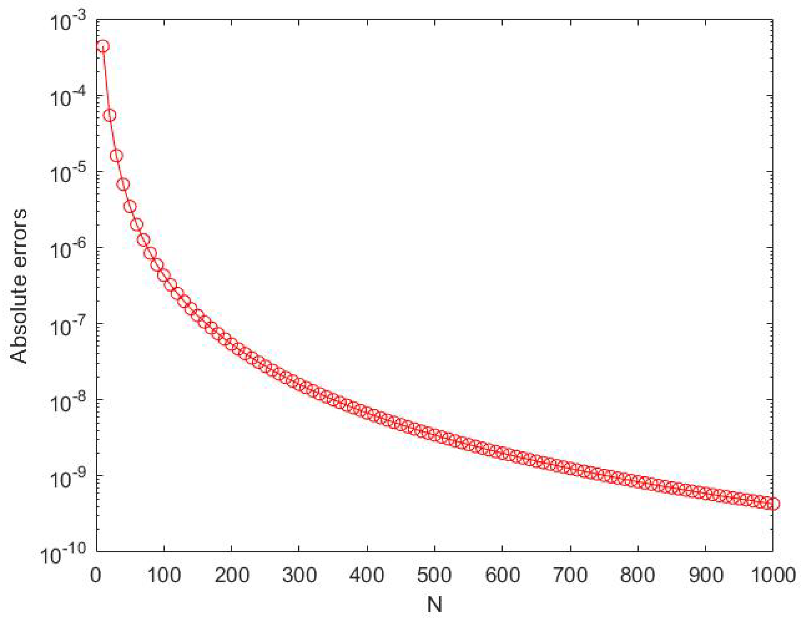
4. Numerical Examples

Example 1.
Let us consider the CSIE of the second kind:
u ( x ) 2 + 1 2 π e i k x 1 1 u ( y ) e i k y y x d y = f ( x ) 2
where f ( x ) = c o s ( x ) . For x = 0.5 and a = b = 1 2 , we get values of α = 0.25 and β = 0.25 from Equation (3) for κ = 0 . The absolute error for u ( x ) is presented in Table 1 and Table 2 below.
Example 2.
The mixed boundary value problem is described in Figure 1.
Taken from [18], it has the analytic solution ϕ ( x , t ) = 2 π a r c t a n 2 y 1 x 2 t 2 . It can further be reduced to the following integral equation for κ = 1 and for α = β = 1 2 .
1 π 1 1 u ( y ) y x d y = C 1 + 1 π 1 x 2 log ( 1 x ) + 1 + x 2 log ( 1 + x ) log ( 2 + x ) 1
Here C 1 is a constant defined as C 1 = 0.4192007182789807 . Furthermore if u ( x ) is known, the solution of the above boundary value can be derived as:
ϕ ( μ , ν ) = 1 π ν u ( y , 0 ) ( y μ ) 2 + ν 2 d y
where:
u ( y , 0 ) = u ( y ) + ( 1 y ) / 2 , | y | 1 , 1 t [ 2 , 1 ] , 0 , o t h e r w i s e .
So here we just solve u ( x ) for simplicity. Figure 2 illustrates the absolute error for u ( x ) .
Figure 2 shows that absolute error for u(x) decreases for greater values of N.
Example 3.
[10,26] For CSIE with k = 0 :
1 1 u ( y ) y x d y = x 4 + 5 x 3 + 2 x 2 + x 11 8
in the case a = 0 and b = 1 , where α and β are derived from Equation (3) and the exact values of u ( y ) for cases κ 0 for the solution bounded at x = 1 , x = 1 , x = ± 1 are given as:
u ( y ) = 1 π 1 + y 1 y y 4 + 4 y 3 5 / 2 y 2 + y 7 / 2 u ( y ) = 1 π 1 y 1 + y y 4 + 6 y 3 + 15 / 2 y 2 + 6 y + 7 / 2 u ( y ) = 1 π 1 y 2 y 3 + 5 y 2 + 5 / 2 y + 7 / 2 .
Table 3 presents the absolute error for the above three cases.
Clearly, Table 3 shows that obtained absolute errors are significantly good for really small values of N, N = 5 , that can never be achieved in [10,26]. The exact value for u ( x ) in the above examples is obtained through Mathematica 11, while the approximated results are calculated using Matlab R2018a on a 4 GHz personal laptop with 8 GB of RAM. For Example 2 Matlab code and Mathematica command is provided as supplementary material.

5. Conclusions

In the presented research work, the Clenshaw–Curtise–Filon quadrature is used to get higher order accuracy. Absolute errors are presented in Table 1 and Table 2 for solutions of highly oscillatory CSIEs for κ = 0 . For larger values of N, Figure 2 shows the absolute error for u ( x ) for mixed the boundary value problem, whereas for frequency k = 0 , the proposed quadrature posseses higher accuracy than the schemes claimed in [10,26]; Table 3 addresses this very well. This shows that the quadrature rule is quite accurate with the exact solution.

Supplementary Materials

Supplementary Materials: The codes are available at https://www.mdpi.com/2227-7390/7/10/872/s1, for Example 2, Figure 2: The absolute error for u(x), for x = 0.6.

Author Contributions

Conceptualization, SAIRA, S.X. and G.L.; Methodology, SAIRA; Supervision, S.X.; Writing (original draft), SAIRA; Writing (review and editing), SAIRA, S.X. and G.L.

Funding

This research received no external funding.

Conflicts of Interest

The authors declare no conflict of interest.

References

  1. Polyanin, A.D.; Manzhirov, A.V. Handbook of Integral Equations; CRC Press: Boca Raton, FL, USA, 1998. [Google Scholar]
  2. Li, J.; Wang, X.; Xiao, S.; Wang, T. A rapid solution of a kind of 1D Fredholm oscillatory integral equation. J. Comput. Appl. Math. 2012, 236, 2696–2705. [Google Scholar] [CrossRef] [Green Version]
  3. Ursell, F. Integral equations with a rapidly oscillating kernel. J. Lond. Math. Soc. 1969, 1, 449–459. [Google Scholar] [CrossRef]
  4. Yalcinbas, S.; Aynigul, M. Hermite series solutions of linear Fredholm integral equations. Math. Comput. Appl. 2011, 16, 497–506. [Google Scholar]
  5. Fang, C.; He, G.; Xiang, S. Hermite-Type Collocation Methods to Solve Volterra Integral Equations with Highly Oscillatory Bessel Kernels. Symmetry 2019, 11, 168. [Google Scholar] [CrossRef]
  6. Babolian, E.; Hajikandi, A.A. The approximate solution of a class of Fredholm integral equations with a weakly singular kernel. J. Comput. Appl. Math. 2011, 235, 1148–1159. [Google Scholar] [CrossRef]
  7. Aimi, A.; Diligenti, M.; Monegato, G. Numerical integration schemes for the BEM solution of hypersingular integral equations. Int. J. Numer. Method Eng. 1999, 45, 1807–1830. [Google Scholar] [CrossRef]
  8. Beyrami, H.; Lotfi, T.; Mahdiani, K. A new efficient method with error analysis for solving the second kind Fredholm integral equation with Cauchy kernel. J. Comput. Appl. Math. 2016, 300, 385–399. [Google Scholar] [CrossRef]
  9. Setia, A. Numerical solution of various cases of Cauchy type singular integral equation. Appl. Math. Comput. 2014, 230, 200–207. [Google Scholar] [CrossRef]
  10. Eshkuvatov, Z.K.; Long, N.N.; Abdulkawi, M. Approximate solution of singular integral equations of the first kind with Cauchy kernel. Appl. Math. Lett. 2009, 22, 651–657. [Google Scholar] [CrossRef] [Green Version]
  11. Cuminato, J.A. Uniform convergence of a collocation method for the numerical solution of Cauchy-type singular integral equations: A generalization. IMA J. Numer. Anal. 1992, 12, 31–45. [Google Scholar] [CrossRef]
  12. Cuminato, J.A. On the uniform convergence of a perturbed collocation method for a class of Cauchy integral equations. Appl. Numer. Math. 1995, 16, 439–455. [Google Scholar] [CrossRef]
  13. Karczmarek, P.; Pylak, D.; Sheshko, M.A. Application of Jacobi polynomials to approximate solution of a singular integral equation with Cauchy kernel. Appl. Math. Comput. 2006, 181, 694–707. [Google Scholar] [CrossRef]
  14. Lifanov, I.K. Singular Integral Equations and Discrete Vortices; Walter de Gruyter GmbH: Berlin, Germany, 1996. [Google Scholar]
  15. Ladopoulos, E.G. Singular Integral Equations: Linear and Non-Linear Theory and Its Applications in Science and Engineering; Springer Science and Business Media: Berlin, Germany, 2013. [Google Scholar]
  16. Muskhelishvili, N.I. Some Basic Problems of the Mathematical Theory of Elasticity; Springer Science and Business Media: Berlin, Germany, 2013. [Google Scholar]
  17. Martin, P.A.; Rizzo, F.J. On boundary integral equations for crack problems. Proc. R. Soc. Lond. A Math. Phys. Sci. 1989, 421, 341–355. [Google Scholar] [CrossRef]
  18. Cuminato, J.A. Numerical solution of Cauchy-type integral equations of index- 1 by collocation methods. Adv. Comput. Math. 1996, 6, 47–64. [Google Scholar] [CrossRef]
  19. Asheim, A.; Huybrechs, D. Complex Gaussian quadrature for oscillatory integral transforms. IMA J. Num. Anal. 2013, 33, 1322–1341. [Google Scholar] [CrossRef] [Green Version]
  20. Chen, R.; An, C. On evaluation of Bessel transforms with oscillatory and algebraic singular integrands. J. Comput. Appl. Math. 2014, 264, 71–81. [Google Scholar] [CrossRef]
  21. Erdelyi, A. Asymptotic representations of Fourier integrals and the method of stationary phase. SIAM 1955, 3, 17–27. [Google Scholar] [CrossRef]
  22. Olver, S. Numerical Approximation of Highly Oscillatory Integrals. Ph.D. Thesis, University of Cambridge, Cambridge, UK, 2008. [Google Scholar]
  23. Milovanovic, G.V. Numerical calculation of integrals involving oscillatory and singular kernels and some applications of quadratures. Comput. Math. Appl. 1998, 36, 19–39. [Google Scholar] [CrossRef] [Green Version]
  24. Dzhishkariani, A.V. The solution of singular integral equations by approximate projection methods. USSR Comput. Math. Math. Phys. 1979, 19, 61–74. [Google Scholar] [CrossRef]
  25. Chakrabarti, A.; Berghe, G.V. Approximate solution of singular integral equations. Appl. Math. Lett. 2004, 17, 553–559. [Google Scholar] [CrossRef] [Green Version]
  26. Dezhbord, A.; Lotfi, T.; Mahdiani, K. A new efficient method for cases of the singular integral equation of the first kind. J. Comput. Appl. Math. 2016, 296, 156–169. [Google Scholar] [CrossRef]
  27. He, G.; Xiang, S. An improved algorithm for the evaluation of Cauchy principal value integrals of oscillatory functions and its application. J. Comput. Appl. Math. 2015, 280, 1–13. [Google Scholar] [CrossRef]
  28. Trefethen, L.N. C hebyshev Polynomials and Series, Approximation theorey and approximation practice. Soc. Ind. Appl. Math. 2013, 128, 17–19. [Google Scholar]
  29. Liu, G.; Xiang, S. Clenshaw Curtis type quadrature rule for hypersingular integrals with highly oscillatory kernels. Appl. Math. Comput. 2019, 340, 251–267. [Google Scholar] [CrossRef]
  30. Wang, H.; Xiang, S. Uniform approximations to Cauchy principal value integrals of oscillatory functions. Appl. Math. Comput. 2009, 215, 1886–1894. [Google Scholar] [CrossRef]
  31. Piessens, R.; Branders, M. On the computation of Fourier transforms of singular functions. J. Comput. Appl. Math. 1992, 43, 159–169. [Google Scholar] [CrossRef] [Green Version]
  32. Oliver, J. The numerical solution of linear recurrence relations. Numer. Math. 1968, 114, 349–360. [Google Scholar] [CrossRef]
  33. Huybrechs, D.; Vandewalle, S. On the evaluation of highly oscillatory integrals by analytic continuation. Siam J. Numer. Anal. 2006, 44, 1026–1048. [Google Scholar] [CrossRef]
  34. Wang, H.; Xiang, S. On the evaluation of Cauchy principal value integrals of oscillatory functions. J. Comput. Appl. Math. 2010, 234, 95–100. [Google Scholar] [CrossRef] [Green Version]
  35. Dominguez, V.; Graham, I.G.; Smyshlyaev, V.P. Stability and error estimates for Filon Clenshaw Curtis rules for highly oscillatory integrals. IMA J. Numer. Anal. 2011, 31, 1253–1280. [Google Scholar] [CrossRef]
  36. Xiang, S.; Chen, X.; Wang, H. Error bounds for approximation in Chebyshev points. Numer. Math. 2010, 116, 463–491. [Google Scholar] [CrossRef]
  37. Xiang, S. Approximation to Logarithmic-Cauchy Type Singular Integrals with Highly Oscillatory Kernels. Symmetry 2019, 11, 728. [Google Scholar] [Green Version]
Figure 1. The mixed boundary value problem.
Mathematics 07 00872 g001
Figure 2. The absolute error for u ( x ) , for x = 0.6 .
Mathematics 07 00872 g002
Table 1. Absolute error for κ = 0 , bounded at x = 1 .
kN = 5N = 10N = 20
504.6387 × 10−93.9207 × 10−141.1102 × 10⁻¹⁶
1001.0881 × 10−94.9564 × 10−150
10003.8093 × 10−114.0030 × 10−162.4825 × 10⁻¹⁶
10,0005.1593 × 10−132.2204 × 10−161.1102 × 10⁻¹⁶
Table 2. Absolute error for κ = 0 , bounded at x = 1 .
kN = 5N = 10N = 20
501.1156 × 10−99.1854 × 10−151.1102 × 10⁻¹⁶
1003.2791 × 10−105.6610 × 10−161.1102 × 10⁻¹⁶
10001.7225 × 10−122.2204 × 10−162.2204 × 10⁻¹⁶
10,0007.3056 × 10−153.3307 × 10−163.3307 × 10⁻¹⁶
Table 3. Absolute error for case κ 0 , k = 0 .
xError
κ = 1 κ = 0 , boundned at x = 1 κ = 0 , boundned at x = 1
−0.601.1102 × 10−164.4409 × 10⁻¹⁶
−0.23.3307 × 10−162.2204 × 10−164.4409 × 10⁻¹⁶
0.22.2204 × 10−164.4409 × 10−160
0.602.2204 × 10−164.4409 × 10⁻¹⁶

