Geometrical Inverse Preconditioning for Symmetric Positive Definite Matrices

Abstract

We focus on inverse preconditioners based on minimizing $F(X)=1-cos(XA,I)$, where $XA$ is the preconditioned matrix and A is symmetric and positive definite. We present and analyze gradient-type methods to minimize $F(X)$ on a suitable compact set. For this, we use the geometrical properties of the non-polyhedral cone of symmetric and positive definite matrices, and also the special properties of $F(X)$ on the feasible set. Preliminary and encouraging numerical results are also presented in which dense and sparse approximations are included.

1. Introduction

The development of algebraic inverse preconditioning continues to be an active research area since they play a key role in a wide variety of applications that involve the solution of large and sparse linear systems of equations; see e.g., [1,2,3,4,5,6,7,8,9,10,11].

A standard and well-known approach to build preconditioning strategies is based on incomplete factorizations of the coefficient matrix: incomplete LU (ILU), incomplete Choleksy (IC), among others. However, preconditioners built with this approach, while popular and fairly easy to implement, are not suitable for parallel platforms, especially Graphics Processing Units (GPUs) [12], and moreover are not always reliable since the incomplete factorization process may yield a very ill-conditioned factorization (see, e.g., [13]). Even for symmetric positive definite matrices, existence of the standard IC factorization is guaranteed only for some special classes of matrices (see, e.g., [14]). In the symmetric positive definite case, variants of IC have been developed to avoid ill-conditioning and breakdown (see, e.g., [15,16]). Nevertheless, usually these modifications are expensive and introduce additional parameters to be chosen in the algorithm.

For a given square matrix A, there exist several proposals for constructing robust sparse inverse approximations which are based on optimization techniques, mainly based on minimizing the Frobenius norm of the residual $(I-XA)$ over a set P of matrices with a certain sparsity pattern; see e.g., [5,6,15,17,18,19,20,21,22]. An advantage of these approximate inverse preconditioners is that the process of building them, as well as applying them, is well suited for parallel platforms. However, we must remark that when A is symmetric and positive definite, minimizing the Frobenius norm of the residual without imposing additional constraints can produce an inverse preconditioner which is neither symmetric nor positive definite; see, e.g., (p. 312 [15]).

There is currently a growing interest, and understanding, in the rich geometrical structure of the non-polyhedral cone of symmetric and positive semidefinite matrices ($PSD$); see e.g., [19,22,23,24,25,26,27]. In this work, we focus on inverse preconditioners based on minimizing the positive-scaling-invariant function $F(X)=1-cos(XA,I)$, instead of minimizing the Frobenius norm of the residual. Our approach takes advantage of the geometrical properties of the $PSD$ cone, and also of the special properties of $F(X)$ on a suitable compact set, to introduce specialized constrained gradient-type methods for which we analyze their convergence properties.

The rest of the document is organized as follows. In Section 2, we develop and analyze two different gradient-type iterative schemes for finding inverse approximations based on minimizing $F(X)$, including sparse versions. In Section 3, we present numerical results on some well-known test matrices to illustrate the behavior and properties of the introduced gradient-type methods. Finally, in Section 4 we present some concluding remarks.

2. Gradient-Type Iterative Methods

Let us recall that the cosine between two $n\times n$ real matrices A and B is defined as

$$cos(A,B)=\frac{\langle A,B\rangle }{{\parallel A\parallel }_F{\parallel B\parallel }_F}$$

(1)

where $\langle A,B\rangle =trace(B^{T}A)$ is the Frobenius inner product in the space of matrices and ${\parallel .\parallel }_F$ is the associated Frobenius norm. By the Cauchy–Schwarz inequality, it follows that

$$|cos(A,B)|\le 1$$

and the equality is attained if and only if $A=\gamma B$ for some nonzero real number γ.

To compute the inverse of a given symmetric and positive definite matrix A, we consider the function

$$F(X)=1-cos(XA,I)\ge 0$$

(2)

for which the minimum value zero is reached at $X=\xi A^{-1}$, for any positive real number ξ. Let us recall that any positive semidefinite matrix B has nonnegative diagonal entries and so $trace(B)\ge 0$. Hence, if $XA$ is symmetric, we need to impose that $\langle XA,I\rangle =trace(XA)\ge 0$ as a necessary condition for $XA$ to be in the $PSD$ cone (see [24,26,27]). Therefore, in order to impose uniqueness in the $PSD$ cone, we consider the constrained minimization problem

$$\underset{X\in S\cap T}{\mathrm{Min}}F(X)$$

(3)

where $S=\{X\in R^{n\times n}|\parallel XA{\parallel }_F=\sqrt{n}\}$ and $T=\{X\in R^{n\times n}|trace(XA)\ge 0\}$. Notice that $S\cap T$ is a closed and bounded set, and so problem (3) is well-posed. Notice also that T is convex while S is not.

Remark 2.1. 

For any $\beta >0$, $F(\beta X)=F(X)$, and so the function F is invariant under positive scaling.

The derivative of $F(X)$, denoted by $\nabla F(X)$, plays an important role in our work.

Lemma 2.1. 

$$\nabla F(X)=\frac{1}{{\parallel I\parallel }_F{\parallel XA\parallel }_F}\left(\frac{\langle XA,I\rangle }{{\parallel XA\parallel }_F^2}XA-I\right)A$$

Proof. 

For fixed matrices X and Y, we consider the function $\phi (t)=F(X+tY)$. It is well-known that ${\phi }^{\prime }(0)=\langle \nabla F(X),Y\rangle$. We have

$$F(X+tY)=1-\frac{1}{{\parallel I\parallel }_F{\parallel XA\parallel }_F}\frac{\langle XA,I\rangle +t\langle YA,I\rangle }{\sqrt{1+2t\frac{\langle XA,YA\rangle }{{\parallel XA\parallel }_F^2}+t^2\frac{{\parallel YA\parallel }^2}{{\parallel XA\parallel }_F^2}}}$$

and we obtain after differentiating $\phi (t)$ and some algebraic manipulations

$${\phi }^{\prime }(0)=\langle \frac{1}{{\parallel I\parallel }_F{\parallel XA\parallel }_F}\left(\frac{\langle XA,I\rangle }{{\parallel XA\parallel }_F^2}XA-I\right)A,Y\rangle$$

and the result is established. ☐

Theorem 2.1. 

Problem (3) possesses the unique solution $X=A^{-1}$.

Proof. 

Notice that $\nabla F(X)=0$ for $X\in S$, if and only if $X=\beta A^{-1}$ for $\beta =\pm 1$. Now, $F(-A^{-1})=2$ and so $X=-A^{-1}$ is the global maximizer of the function F on S, but $-A^{-1}\notin T$; however, $F(A^{-1})=0$ and $A^{-1}\in T$. Therefore, $X=A^{-1}$ is the unique feasible solution of (3). ☐

Before discussing different numerical schemes for solving problem (3), we need a couple of technical lemmas.

Lemma 2.2. 

If $X\in S$ and $XA=AX$, then

$$\langle \nabla F(X),X\rangle =0$$

Proof. 

Since $X\in S$ then ${\parallel XA\parallel }_F^2=n$, and we have

$$\nabla F(X)=\frac{1}{n}\left(\frac{\langle XA,I\rangle }{n}XA-I\right)A$$

hence

$$\langle \nabla F(X),X\rangle =\frac{1}{n}\frac{\langle XA,I\rangle }{n}\langle XAA,X\rangle -\frac{1}{n}\langle A,X\rangle$$

However, $\langle XAA,X\rangle ={\parallel XA\parallel }_F^2=n$, so

$$\langle \nabla F(X),X\rangle =\frac{\langle XA,I\rangle }{n}-\frac{1}{n}\langle A,X\rangle =0$$

since $\langle A,X\rangle =\langle AX,I\rangle =\langle XA,I\rangle$. ☐

Lemma 2.3. 

If $X\in S$, then

$$\frac{\sqrt{n}}{{\parallel A\parallel }_F}\le {\parallel X\parallel }_F\le \sqrt{n}{\parallel A^{-1}\parallel }_F$$

Proof. 

For every X, we have $X=A^{-1}AX$, and so

$${\parallel X\parallel }_F=\parallel A^{-1}{AX\parallel }_F\le \sqrt{n}{\parallel A^{-1}\parallel }_F$$

On the other hand, since $X\in S$, $\sqrt{n}={\parallel XA\parallel }_F\le {\parallel X\parallel }_F{\parallel A\parallel }_F$, and hence

$${\parallel X\parallel }_F\ge \frac{\sqrt{n}}{{\parallel A\parallel }_F}$$

and the result is established. ☐

2.1. The Negative Gradient Direction

For the numerical solution of (3), we start by considering the classical gradient iterations that, from an initial guess $X_0$, are given by

$$X^{(k+1)}=X^{(k)}-{\alpha }_k\nabla F(X^{(k)})$$

where ${\alpha }_k>0$ is a suitable step length. A standard approach is to use the optimal choice i.e., the positive step length that (exactly) minimizes the function $F(X)$ along the negative gradient direction. We present a closed formula for the optimal choice of step length in a more general setting, assuming that the iterative method is given by:

$$X^{(k+1)}=X^{(k)}+{\alpha }_k{D}_k$$

where $D_k$ is a search direction in the space of matrices.

Lemma 2.4. 

The optimal step length ${\alpha }_k$, that optimizes $F(X^{(k)}+\alpha D_k)$, is given by

$${\alpha }_k=\frac{\left(\langle X^{(k)}A,I\rangle \langle X^{(k)}A,D_{k}A\rangle -n\langle D_{k}A,I\rangle \right)}{\left(\langle D_{k}A,I\rangle \langle X^{(k)}A,D_{k}A\rangle -\langle X^{(k)}A,I\rangle \langle D_{k}A,D_{k}A\rangle \right)}$$

Proof. 

Consider the auxiliary function in one variable

$$\psi (\alpha )=F(X^{(k)}+\alpha D_k)=1-\frac{\langle X^{(k)}A,I\rangle +\alpha \langle D_{k}A,I\rangle }{\sqrt{n}{\parallel X^{(k)}A+\alpha D_{k}A\parallel }_F}$$

Differentiating $\psi (\alpha )$, using that $\langle X^{(k)}A,X^{(k)}A\rangle =n$, and also that

$$\frac{\partial }{\partial \alpha }{\parallel X^{(k)}A+\alpha D_{k}A\parallel }_F=\frac{\langle X^{(k)}A,D_{k}A\rangle +\alpha \langle D_{k}A,D_{k}A\rangle }{\parallel X^{(k)}A+\alpha D_k{A\parallel }_F}$$

and then forcing ${\psi }^{\prime }(\alpha )=0$ the result is obtained, after some algebraic manipulations. ☐

Remark 2.2. 

For our first approach, $D_k=-\nabla F(X^{(k)})$, and so for the optimal gradient method (also known as Cauchy method or steepest descent method) the step length is given by

$${\alpha }_k=\frac{\left(n\langle \nabla F(X^{(k)})A,I\rangle -\langle X^{(k)}A,I\rangle \langle X^{(k)}A,\nabla F(X^{(k)})A\rangle \right)}{\left(\langle \nabla F(X^{(k)})A,I\rangle \langle X^{(k)}A,\nabla F(X^{(k)})A\rangle -\langle X^{(k)}A,I\rangle {\parallel \nabla F(X^{(k)})A\parallel }_F^2\right)}$$

(4)

Notice that if instead of using the descent direction $D_k=-\nabla F(X^{(k)})$, we use the ascent direction $D_k=\nabla F(X^{(k)})$, in Lemma 2.4, the obtained ${\alpha }_k$ that also forces ${\psi }^{\prime }({\alpha }_k)=0$, is given by (4) but with a negative sign in front. Hence, to guarantee that the step length ${\alpha }_k$ is positive to minimize F along the negative gradient direction to approximate $A^{-1}$, instead of maximizing F along the gradient direction to approximate $-A^{-1}$, we will choose the step length ${\alpha }_k$ as the absolute value of the expression in (4).

Since ${\parallel I\parallel }_F=\sqrt{n}$, the gradient iterations can be written as

$$X^{(k+1)}=X^{(k)}-\frac{{\alpha }_k}{\sqrt{n}{\parallel X^{(k)}A\parallel }_F}\left(\frac{\langle X^{(k)}A,I\rangle }{\parallel X^{(k)}{A\parallel }_F^2}{X}^{(k)}A-I\right)A$$

which can be further simplified by imposing the condition for uniqueness $\parallel X^{(k)}{A\parallel }_F=\sqrt{n}$. In that case, we set

$$Z^{(k+1)}=X^{(k)}-\frac{{\alpha }_k}{n}\left(\frac{\langle X^{(k)}A,I\rangle }{n}{X}^{(k)}A-I\right)A$$

(5)

and then we multiply the matrix $Z^{(k+1)}$ by the factor $\sqrt{n}/{\parallel Z^{(k+1)}A\parallel }_F$ to guarantee that $X^{(k+1)}\in S$, i.e., such that $\parallel X^{(k+1)}{A\parallel }_F=\sqrt{n}$.

Concerning the condition that the sequence $\{X^{(k)}\}$ remains in T, in our next result, we establish that if the step length ${\alpha }_k$ remains uniformly bounded from above, then $trace(X^{(k)}A)>0$ for all k.

Lemma 2.5. 

Assume that $trace(X^{(0)}A)>0$ and that $0<{\alpha }_k\le \frac{n^{3/2}}{{\parallel A\parallel }_F^2}$. Then,

$$trace(X^{(k)}A)=\langle X^{(k)}A,I\rangle >0for all k$$

Proof. 

We proceed by induction. Let us assume that

$$w_k:=trace(X^{(k)}A)=\langle X^{(k)}A,I\rangle >0$$

It follows that

$$Z^{(k+1)}A=X^{(k)}A-\frac{{\alpha }_k}{n}\left(\frac{w_k}{n}{X}^{(k)}A-I\right)A^2$$

and so

$$trace(Z^{(k+1)}A)=w_k-\frac{{\alpha }_k}{n}\left(\frac{w_k}{n}trace(X^{(k)}{A}^3)-trace(A^2)\right)$$

Now, since $trace(A^2)=\langle A,A\rangle ={\parallel A\parallel }_F^2$ and

$$trace(X^{(k)}{A}^3)\le \parallel X^{(k)}{A\parallel }_F{\parallel A\parallel }_F^2=\sqrt{n}{\parallel A\parallel }_F^2$$

we obtain that

$$trace(Z^{(k+1)}A)\ge (1-\frac{{\alpha }_k}{n^2}\sqrt{n}{\parallel A\parallel }_F^2)w_k+\frac{{\alpha }_k}{n}{\parallel A\parallel }_F^2$$

Since $0<{\alpha }_k\le \frac{n^{3/2}}{{\parallel A\parallel }_F^2}$, then $(1-\frac{{\alpha }_k}{n^2}\sqrt{n}\parallel A{\parallel }_F^2)>0$, and we conclude that

$$trace(Z^{(k+1)}A)>0$$

Since $X^{(k+1)}$ is obtained as a positive scaling factor of $Z^{(k+1)}$, then $w_{k+1}>0$, and the result is established. ☐

Now, for some given matrices A, we cannot guarantee that the step length computed as the absolute value of (4) will satisfy ${\alpha }_k\le (n^{3/2})/{\parallel A\parallel }_F^2$ for all k. Therefore, if $trace(X^{(k+1)}A)=\langle X^{(k+1)}A,I\rangle <0$, then we will set in our algorithm $X^{(k+1)}=-X^{(k+1)}$ to guarantee that $trace(X^{(k+1)}A)\ge 0$, and hence that the cosine between $X^{(k+1)}A$ and I is nonnegative, which is a necessary condition to guarantee that $X^{(k+1)}$ remains in the $PSD$ cone (see, e.g., [24,26,27].

We now present our steepest descent gradient algorithm that will be referred as the CauchyCos Algorithm.

Algorithm 1 : CauchyCos (Steepest descent approach on CauchyCos (Steepest descent approach on $F(X)=1-cos(XA,I)$)

1: Given $X_0\in PSD$ 2: for $k=0,1,\cdots$ until a stopping criterion is satisfied, do 3:  Set $w_k=\langle X^{(k)}A,I\rangle$ 4:  Set $\nabla F(X^{(k)})=\frac{1}{n}\left(\frac{w_k}{n}{X}^{(k)}A-I\right)A$ 5:  Set ${\alpha }_k=\left|\frac{n\langle \nabla F(X^{(k)})A,I\rangle -w_k\langle X^{(k)}A,\nabla F(X^{(k)})A\rangle }{\langle \nabla F(X^{(k)})A,I\rangle \langle X^{(k)}A,\nabla F(X^{(k)})A\rangle -w_k{\parallel \nabla F(X^{(k)})A\parallel }_F^2}\right|$ 6:  Set $Z^{(k+1)}=X^{(k)}-{\alpha }_k\nabla F(X^{(k)})$ 7:  Set $X^{(k+1)}=s\sqrt{n}\frac{Z^{(k+1)}}{\parallel Z^{(k+1)}{A\parallel }_F}$, where $s=1$ if $trace(Z^{(k+1)}A)>0$, $s=-1$ else 8: end for

We note that if we start from $X^{(0)}$ such that $\parallel X^{(0)}{A\parallel }_F=\sqrt{n}$ then by construction $\parallel X^{(k)}{A\parallel }_F=\sqrt{n}$, for all $k\ge 0$; for example, $X^{(0)}=(\sqrt{n}/{\parallel A\parallel }_F)I$ is a convenient choice. For that initial guess, $trace(X^{(0)}A)=\langle X^{(0)}A,I\rangle >0$ and again by construction all the iterates will remain in the $PSD$ cone. Notice also that, at each iteration, we need to compute the three matrix–matrix products: $X^{(k)}A$, $(\frac{w_k}{n}{X}^{(k)}A-I)A$, and $\nabla F(X^{(k)})A$, which, for dense matrices, require $n^3$ floating point operations (flops) each. Every one of the remaining calculations (inner products and Frobenius norms) are obtained with n column-oriented inner products that require n flops each. Summing up, in the dense case, the computational cost of each iteration of the CauchyCos Algorithm is $3n^3+O(n^2)$ flops. In Section 2.5, we will discuss a sparse version of the CauchyCos Algorithm and its computational cost.

2.2. Convergence Properties of the CauchyCos Algorithm

In spite of the resemblance with the classical Cauchy method for convex constrained optimization, the CauchyCos algorithm involves certain key ingredients in its formulation that splits it apart from the Cauchy method. Therefore, a specialized convergence analysis is required. In particular, we note that the constraint set S on which the iterates are computed, thanks to the scaling step 7, is not a convex set.

We start by establishing the commutativity of all iterates with the matrix A.

Lemma 2.6. 

If $X^{(0)}A=A{X}^{(0)}$, then $X^{(k)}A=A{X}^{(k)}$, for all $k\ge 0$ in the CauchyCos Algorithm. Furthermore, if $X^{(0)}$ is symmetric, then $X^{(k)}$ and $X^{(k)}A$ are symmetric for all $k\ge 0$.

Proof. 

We proceed by induction. Assume that $X^{(k)}A=A{X}^{(k)}$. It follows that:

$$\begin{array}{cc}\hfill A{Z}^{(k+1)}& =A{X}^{(k)}-\frac{{\alpha }_k}{n}\left(\frac{\langle X^{(k)}A,I\rangle }{n}A{X}^{(k)}A-A\right)A\hfill \\ & =X^{(k)}A-\frac{{\alpha }_k}{n}\left(\frac{\langle X^{(k)}A,I\rangle }{n}A{X}^{(k)}-I\right)AA\hfill \\ & =\left(X^{(k)}-\frac{{\alpha }_k}{n}\left(\frac{\langle X^{(k)}A,I\rangle }{n}{X}^{(k)}A-I\right)A\right)A\hfill \\ & =Z^{(k+1)}A\hfill \end{array}$$

and since $Z^{(k+1)}$ and $X^{(k+1)}$ differ only by a scaling factor, then $A{X}^{(k+1)}=X^{(k+1)}A$. Hence, since $X^{(0)}A=A{X}^{(0)}$, the result holds for all k. The second property is proven similarly by induction. ☐

It is worth noticing that, using Lemma 2.6 and (5), it follows by simple calculations that $Z^{(k)}$ as well as $X^{(k)}$ are symmetric matrices for all k. In turn, if $X^{(0)}A=A{X}^{(0)}$, this clearly implies using Lemma 2.6 that $X^{(k)}A$ is also a symmetric matrix for all k.

Our next result establishes that the sequences generated by the CauchyCos Algorithm are uniformly bounded away from zero, and hence the algorithm is well-defined.

Lemma 2.7. 

If $X^{(0)}A=A{X}^{(0)}$, then the sequences $\left\{X^{(k)}\right\}$, $\left\{Z^{(k)}\right\}$, and $\left\{Z^{(k)}A\right\}$ generated by the CauchyCos Algorithm are uniformly bounded away from zero.

Proof. 

Using Lemmas 2.2 and 2.6 we have that

$$\langle Z^{(k+1)},X^{(k)}\rangle =\parallel X^{(k)}{\parallel }_F^2-{\alpha }_k\langle \nabla F(X^{(k)}),X^{(k)}\rangle ={\parallel X^{(k)}\parallel }_F^2$$

which combined with the Cauchy–Schwarz inequality and Lemma 2.3 implies that

$$\parallel Z^{(k+1)}{\parallel }_F\ge {\parallel X^{(k)}\parallel }_F\ge \frac{\sqrt{n}}{{\parallel A\parallel }_F}>0$$

for all k. Moreover, since A is nonsingular then

$$\parallel Z^{(k+1)}{A\parallel }_F\ge \frac{\parallel Z^{(k+1)}{\parallel }_F}{\parallel A^{-1}{\parallel }_F}\ge \frac{\sqrt{n}}{{\parallel A\parallel }_F{\parallel A^{-1}\parallel }_F}>0$$

is bounded away from zero for all k. ☐

Theorem 2.2. 

The sequence $\left\{X^{(k)}\right\}$ generated by the CauchyCos Algorithm converges to $A^{-1}$.

Proof. 

The sequence $\left\{X^{(k)}\right\}\subset S\cap T$, which is a closed and bounded set; therefore, there exist limit points in $S\cap T$. Let $\widehat{X}$ be a limit point of $\left\{X^{(k)}\right\}$, and let $\left\{X^{(k_j)}\right\}$ be a subsequence that converges to $\widehat{X}$. Let us suppose, by way of contradiction, that $\nabla F(\widehat{X})\ne 0$.

In that case, the negative gradient, $-\nabla F(\widehat{X})\ne 0$, is a descent direction for the function F at $\widehat{X}$. Hence, there exists $\widehat{\alpha }>0$ such that

$$\delta =F(\widehat{X})-F(\widehat{X}-\widehat{\alpha }\nabla F(\widehat{X}))>0$$

Consider now an auxiliary function $\theta :R^{n\times n}\to R$ given by

$$\theta (X)=F(X)-F(X-\widehat{\alpha }\nabla F(X))$$

Clearly, θ is a continuous function, and then $\theta (X^{(k_j)})$ converges to $\theta (\widehat{X})=\delta$. Therefore, for all $k_j$ sufficiently large,

$$F(X^{(k_j)})-F(X^{(k_j)}-\widehat{\alpha }\nabla F(X^{(k_j)}))=\theta (X^{(k_j)})\ge \delta /2$$

Now, since ${\alpha }_{k_j}$ was obtained using Lemma 2.4 as the exact optimal step length along the negative gradient direction, then using Remark 2.1, it follows that

$$\begin{array}{ccc}\hfill F(X^{(k_j+1)})=F(Z^{(k_j+1)})& =& F(X^{(k_j)}-{\alpha }_{k_j}\nabla F(X^{(k_j)}))\hfill \\ & <& F(X^{(k_j)}-\widehat{\alpha }\nabla F(X^{(k_j)}))\le F(X^{(k_j)})-\frac{\delta }{2}\hfill \end{array}$$

and thus,

$$F(X^{(k_j)})-F(X^{(k_j+1)})\ge \frac{\delta }{2}$$

(6)

for all $k_j$ sufficiently large.

On the other hand, since F is continuous, $F(X^{(k_j)})$ converges to $F(\widehat{X})$. However, the whole sequence $\left\{F(X^{(k)})\right\}$ generated by the CauchyCos Algorithm is decreasing, and so $F(X^{(k)})$ converges to $F(\widehat{X})$, and since F is bounded below then for $k_j$ large enough

$$F(X^{(k_j)})-F(X^{(k_j+1)})\to 0$$

which contradicts (6). Consequently, $\nabla F(\widehat{X})=0$.

Now, using Lemma 2.1, it follows that $\nabla F(\widehat{X})=0$ implies $\widehat{X}=A^{-1}$. Hence, the subsequence $\left\{X^{(k_j)}\right\}$ converges to $A^{-1}$. Nevertheless, as we argued before, the whole sequence $F(X^{(k)})$ converges to $F(A^{-1})=0$, and by continuity the whole sequence $\left\{X^{(k)}\right\}$ converges to $A^{-1}$. ☐

Notice that Theorem 2.2 states that the sequence $X^{(k)}$ converges to $A^{-1}$ which is in the $PSD$ cone. Hence, if $X^{(0)}$ is symmetric and $X^{(0)}A=A{X}^{(0)}$, then $X^{(k)}A$ is symmetric (Lemma 2.6), and after a k iterations (k large enough), the eigenvalues of $X^{(k)}A$ are strictly positive: as a consequence, $X^{(k)}A$ is in the $PSD$ cone.

Remark 2.3. 

The optimal choice of step length ${\alpha }_k$, as it usually happens when combined with the negative gradient direction (see e.g., [28,29]), produces an orthogonality between consecutive gradient directions, that in our setting becomes $\langle \nabla F(Z^{(k+1)}),\nabla F(X^{(k)})\rangle =0$. Indeed, ${\alpha }_k$ minimizes $\psi (\alpha )=F(X^{(k)}-\alpha \nabla F(X^{(k)}))$, which means that

$$0={\psi }^{\prime }({\alpha }_k)=-\langle \nabla F(X^{(k)}-\alpha \nabla F(X^{(k)})),\nabla F(X^{(k)})\rangle =-\langle \nabla F(Z^{(k+1)}),\nabla F(X^{(k)})\rangle$$

This orthogonality is responsible for the well-known zig-zagging behavior of the optimal gradient method, which in some cases induces a very slow convergence.

2.3. A Simplified Search Direction

To avoid the zig-zagging trajectory of the optimal gradient iterates, we now consider a different search direction:

$${\widehat{D}}_k\equiv \widehat{D}(X^{(k)})=-\frac{1}{n}\left(\frac{\langle X^{(k)}A,I\rangle }{n}{X}^{(k)}A-I\right)$$

(7)

to move from $X^{(k)}\in S\cap T$ to the next iterate. Notice that ${\widehat{D}}_{k}A=-\nabla F(X^{(k)})$ and so ${\widehat{D}}_k$ can be viewed as a simplified version of the search direction used in the classical steepest descent method. Moreover, the direction ${\widehat{D}}_k$ in (7) is obtained from the direction $D_k$ used by CauchyCos by multiplying on the right by the matrix ${(A)}^{-1}$, so it can be viewed as a right-preconditioning of the method CauchyCos. Notice also that ${\widehat{D}}_k$ resembles the residual direction $(X^{(k)}A-I)$ used in the minimal residual iterative method (MinRes) for minimizing ${\parallel I-XA\parallel }_F$ in the least-squares sense (see e.g., [6,10]). Nevertheless, the scaling factors in (7) differ from the scaling factors in the classical residual direction at $X^{(k)}$. Note that MinRes here should not be confused with the Krylov method MINRES [10].

For solving (3), we now present a variation of the CauchyCos Algorithm, that will be referred as the MinCos Algorithm, which from a given initial guess $X_0$ produces a sequence of iterates using the search direction ${\widehat{D}}_k$, while remaining in the compact set $S\cap T$. This new algorithm consists of simply replacing $-\nabla F(X^{(k)})$ in the CauchyCos Algorithm by ${\widehat{D}}_k$.

Algorithm 2 : MinCos (simplified gradient approach on $F(X)=1-cos(XA,I)$)

1: Given $X_0\in PSD$ 2: for $k=0,1,\cdots$ until a stopping criterion is satisfied, do 3:  Set $w_k=\langle X^{(k)}A,I\rangle$ 4:  Set ${\widehat{D}}_k=-\frac{1}{n}\left(\frac{w_k}{n}{X}^{(k)}A-I\right)$ 5:  Set ${\alpha }_k=\left|\frac{n\langle {\widehat{D}}_{k}A,I\rangle -w_k\langle X^{(k)}A,{\widehat{D}}_{k}A\rangle }{\langle {\widehat{D}}_{k}A,I\rangle \langle X^{(k)}A,{\widehat{D}}_{k}A\rangle -w_k{\parallel {\widehat{D}}_{k}A\parallel }_F^2}\right|$ 6:  Set $Z^{(k+1)}=X^{(k)}+{\alpha }_k{\widehat{D}}_k$ 7:  Set $X^{(k+1)}=s\sqrt{n}\frac{Z^{(k+1)}}{\parallel Z^{(k+1)}{A\parallel }_F}$, where $s=1$ if $trace(Z^{(k+1)}A)>0$, $s=-1$ else 8: end for

As before, we note that if we start from $X^{(0)}=(\sqrt{n}/{\parallel A\parallel }_F)I$ then by construction $\parallel X^{(k)}{A\parallel }_F=\sqrt{n}$, for all $k\ge 0$. For that initial guess, $trace(X^{(0)}A)=\langle X^{(0)}A,I\rangle >0$ and again by construction all the iterates remain in the $PSD$ cone. Notice also that, at each iteration, we now need to compute the two matrix–matrix products: $X^{(k)}A$, and ${\widehat{D}}_{k}A$, which for dense matrices require $n^3$ flops each. Every one of the remaining calculations (inner products and Frobenius norms) are obtained with n column-oriented inner products that require n flops each. Summing up, in the dense case, the computational cost of each iteration of the MinCos Algorithm is $2n^3+O(n^2)$ flops. In Section 2.5, we will discuss a sparse version of the MinCos Algorithm and its computational cost.

2.4. Convergence Properties of the MinCos Algorithm

We start by noticing that, unless we are at the solution, the search direction ${\widehat{D}}_k$ is a descent direction.

Lemma 2.8. 

If $X\in S\cap T$ and $\nabla F(X)\ne 0$, the search direction $\widehat{D}(X)$ is a descent direction for the function F at X.

Proof. 

We need to establish that, for a given $X\in S\cap T$, $\langle \widehat{D}(X),\nabla F(X)\rangle <0$. Since $A^{-1}$ is symmetric and positive definite, then it has a unique square root which is also symmetric and positive definite. This particular square root will be denoted as $A^{-1/2}$. Therefore, since $\widehat{D}(X)A=-\nabla F(X)$, and using that $trace(E_1{E}_2)=trace(E_2{E}_1)$, for given square matrices $E_1$ and $E_2$, it follows that

$$\begin{array}{ccc}\hfill \langle \widehat{D}(X),\nabla F(X)\rangle & =& \langle \widehat{D}(X)A{A}^{-1},\nabla F(X)\rangle =-\langle \nabla F(X)A^{-1},\nabla F(X)\rangle \hfill \\ & =& -\langle \nabla F(X)A^{-1/2},\nabla F(X)A^{-1/2}\rangle =-{\parallel \nabla F(X)A^{-1/2}\parallel }_F^2<0\hfill \end{array}$$

☐

Remark 2.4. 

The step length in the MinCos Algorithm is obtained using the search direction ${\widehat{D}}_k$ in Lemma (2.4). Notice that if we use $-{\widehat{D}}_k$ instead of ${\widehat{D}}_k$, the obtained ${\alpha }_k$ which also forces ${\psi }^{\prime }({\alpha }_k)=0$ is the one given by Lemma (2.4) but with a negative sign. Therefore, as in the CauchyCos Algorithm, to guarantee that ${\alpha }_k>0$ minimizes F along the descent direction ${\widehat{D}}_k$ to approximate $A^{-1}$, instead of maximizing F along the ascent direction $-{\widehat{D}}_k$ to approximate $-A^{-1}$, we choose the step length ${\alpha }_k$ as the absolute value of the expression in Lemma (2.4).

We now establish the commutativity of all iterates with the matrix A.

Lemma 2.9. 

If $X^{(0)}A=A{X}^{(0)}$, then $X^{(k)}A=A{X}^{(k)}$, for all $k\ge 0$ in the MinCos Algorithm.

Proof. 

We proceed by induction. Assume that $X^{(k)}A=A{X}^{(k)}$. We have that

$$\begin{array}{cc}A{Z}^{(k+1)}\hfill & =A{X}^{(k)}-\frac{{\alpha }_k}{n}\left(\frac{\langle X^{(k)}A,I\rangle }{n}A{X}^{(k)}A-A\right)\hfill \\ & =X^{(k)}A-\frac{{\alpha }_k}{n}\left(\frac{\langle X^{(k)}A,I\rangle }{n}A{X}^{(k)}-I\right)A\hfill \\ & =\left(X^{(k)}-\frac{{\alpha }_k}{n}\left(\frac{\langle X^{(k)}A,I\rangle }{n}{X}^{(k)}A-I\right)A\right)\hfill \\ & =Z^{(k+1)}A\hfill \end{array}$$

and since $Z^{(k+1)}$ and $X^{(k+1)}$ differ only by a scaling factor, then $A{X}^{(k+1)}=X^{(k+1)}A$. Hence, since $X^{(0)}A=A{X}^{(0)}$, the result holds for all k. ☐

It is worth noticing that using Lemma 2.9 and (5), it follows by simple calculations that $Z^{(k)}$, $X^{(k)}$, and $X^{(k)}A$ in the MinCos Algorithm are symmetric matrices for all k. These three sequences generated by the MinCos Algorithm are also uniformly bounded away from zero, and so the algorithm is well-defined.

Lemma 2.10. 

If $X^{(0)}A=A{X}^{(0)}$, then the sequences $\left\{X^{(k)}\right\}$, $\left\{Z^{(k)}\right\}$, and $\left\{Z^{(k)}A\right\}$ generated by the MinCos Algorithm are uniformly bounded away from zero.

Proof. 

From Lemma 2.3, the sequence $\left\{X^{(k)}\right\}$ is uniformly bounded. For the sequence $\left\{Z^{(k)}\right\}$, using Lemmas 2.2 and 2.9, we have that

$$\begin{array}{ccc}\hfill \langle Z^{(k+1)}{A}^{1/2},X^{(k)}{A}^{1/2}\rangle & =& \langle Z^{(k+1)}A,X^{(k)}\rangle =\langle X^{(k)}A,X^{(k)}\rangle +{\alpha }_k\langle D_{k}A,X^{(k)}\rangle \hfill \\ & =& \langle X^{(k)}A,X^{(k)}\rangle -{\alpha }_k\langle \nabla F(X^{(k)}),X^{(k)}\rangle =\langle X^{(k)}A,X^{(k)}\rangle \hfill \\ & =& \langle X^{(k)}{A}^{1/2},X^{(k)}{A}^{1/2}\rangle ={\parallel X^{(k)}{A}^{1/2}\parallel }_F^2\hfill \end{array}$$

where $A^{1/2}$ is the unique square root of A, which is also symmetric and positive definite. Combining the previous equality with the Cauchy–Schwarz inequality, and using the consistency of the Frobenius norm, we obtain

$$\parallel Z^{(k+1)}{\parallel }_F\parallel A^{1/2}{\parallel }_F\ge \parallel Z^{(k+1)}{A}^{1/2}{\parallel }_F\ge {\parallel X^{(k)}{A}^{1/2}\parallel }_F$$

(8)

Since $X^{(k)}\in S$, then $\sqrt{n}=\parallel X^{(k)}{A\parallel }_F\le \parallel X^{(k)}{A}^{1/2}{\parallel }_F{\parallel A^{1/2}\parallel }_F$, which combined with (8) implies that

$$\parallel Z^{(k+1)}{\parallel }_F\ge \frac{\sqrt{n}}{\parallel A^{1/2}{\parallel }_F^2}>0$$

is bounded away from zero for all k. Moreover, since A is nonsingular then

$$\parallel Z^{(k+1)}{A\parallel }_F\ge \frac{\parallel Z^{(k+1)}{\parallel }_F}{\parallel A^{-1}{\parallel }_F}\ge \frac{\sqrt{n}}{\parallel A^{1/2}{\parallel }_F^2{\parallel A^{-1}\parallel }_F}>0$$

is also bounded away from zero for all k. ☐

Theorem 2.3. 

The sequence $\left\{X^{(k)}\right\}$ generated by the MinCos Algorithm converges to $A^{-1}$.

Proof. 

From Lemma 2.8, the search direction $\widehat{D}(X)$ is a descent direction for F at X, unless $\nabla F(X)=0$. Therefore, since ${\alpha }_k$ in the MinCos Algorithm is obtained as the exact minimizer of F along the direction $D(X_k)$ for all k, the proof is obtained repeating the same arguments shown in the proof of Theorem 2.2, simply replacing $-\nabla F(Y)$ by $D(Y)$ for all possible instances Y. ☐

2.5. Connections between the Considered Methods and Sparse Versions

For a given matrix A, the merit function $\Phi (X)=\frac{1}{2}{\parallel I-XA\parallel }_F^2$ has been widely used for computing approximate inverse preconditioners (see, e.g., [5,6,15,17,18,19,20,22]). In that case, the properties of the Frobenius norm permit in a natural way the use of parallel computing. Moreover, the minimization of $\Phi (X)$ can also be accomplished imposing a column-wise numerical dropping strategy leading to a sparse approximation of $A^{-1}$. Therefore, when possible, it is natural to compare the CauchyCos and the MinCos Algorithms applied to the angle-related merit function $F(X)$ with the optimal Cauchy method applied to $\Phi (X)$ (referred from now on as the CauchyFro method), and also to the Minimal Residual (MinRes) method applied to $\Phi (X)$ (see, e.g., [6,15]). Notice that, as we mentioned before in Section 2.3, with respect to CauchyCos and MinCos, MinRes can be seen as a right-preconditioning version of the method CauchyFro.

The gradient of $\Phi (X)$ is given by $\nabla \Phi (X)=-A^T(I-XA)$, and so the iterations of the CauchyFro method, from the same initial guess $X^{(0)}=(\sqrt{n}/{\parallel A\parallel }_F)I$ used by MinCos and CauchyCos, can be written as

$$X^{(k+1)}=X^{(k)}+{\alpha }_k{G}_k$$

(9)

where $G_k=-\nabla \Phi (X^{(k)})$ and the step length ${\alpha }_k>0$ is obtained as the global minimizer of $\Phi (X^{(k)}+\alpha G_k)$ along the direction $G_k$, as follows

$${\alpha }_k=\frac{\langle R_k,A{G}_k\rangle }{\langle A{G}_k,A{G}_k\rangle }$$

(10)

where $R_k=I-A{X}^{(k)}$ is the residual matrix at $X^{(k)}$. The iterations of the MinRes method can be obtained replacing $G_k$ by the residual matrix $R_k$ in (9) and (10) (see [6] for details). We need to remark that in the dense case, the CauchyFro method needs to compute two matrix-matrix products per iteration, whereas the MinRes method by using the recursion $R_{k+1}=R_k-{\alpha }_{k}A{R}_k$ needs one matrix-matrix product per iteration.

We now discuss how to dynamically impose sparsity in the sequence of iterates $\left\{X^{(k)}\right\}$ generated by either the CauchyCos Algorithm or the MinCos Algorithm, to reduce their required storage and computational cost.

A possible way of accomplishing this task is to prescribe a sparsity pattern beforehand, which is usually related to the sparsity pattern of the original matrix A, and then impose it at every iteration (see e.g., [4,20,21,22]). At this point, we would like to mention that although there exist some special applications for which the involved matrices are large and dense [30,31], frequently in real applications the involved matrices are large and sparse. However, in general, the inverse of a sparse matrix is dense anyway. Moreover, with very few exceptions, it is not possible to know a priori the location of the large or the small entries of the inverse. Consequently, it is very difficult in general to prescribe a priori a nonzero sparsity pattern for the approximate inverse.

As a consequence, to force sparsity in our gradient related algorithms, we use instead a numerical dropping strategy to each column (or row) independently, using a threshold tolerance, combined with a fixed bound on the maximum number of nonzero elements to be kept at each column (or row) to limit the fill-in. This combined strategy will be fully described in our numerical results section.

In the CauchyCos and MinCos Algorithms, the dropping strategy must be applied to the matrix $Z_{k+1}$ right after it is obtained at Step 6, and before computing $X_{k+1}$ at Step 7. That way, $X_{k+1}$ will remain sparse at all iterations, and we guarantee that $X_{k+1}\in S\cap T$. The new Steps 7 and 8, in the sparse versions of both algorithms, are given by

7:

Apply numerical dropping to $Z^{(k+1)}$ with a maximum number of nonzero entries;

8:

Set $X^{(k+1)}=s\sqrt{n}\frac{Z^{(k+1)}}{\parallel Z^{(k+1)}{A\parallel }_F}$, where $s=1$ if $trace(Z^{(k+1)}A)>0$, $s=-1$ else.

Notice that, since all the involved matrices are symmetric, the matrix-matrix products required in both algorithms can be performed using sparse-sparse mode column-oriented inner products (see, e.g., [6]). The remaining calculations (inner products and Frobenius norms), required to obtain the step length, must be also computed using sparse-sparse mode. Using this approach, which takes advantage of the imposed sparsity, the computational cost and the required storage of both algorithms are drastically reduced. Moreover, using the column oriented approach both algorithms have a potential for parallelization.

3. Numerical Results

We present some numerical results to illustrate the properties of our gradient-type algorithms for obtaining inverse approximations. All computations are performed in MATLAB using double precision. To test the robustness of our methods, we present hereafter a variety of problems with large scale matrices and very badly conditioned ones (non necessarily of big size) but for which the building of an approximate inverse is difficult. Most of the matrices are taken from the Matrix Market collection [32], which contains a large choice of benchmarks that are widely used.

It is worth mentioning that Schulz method [33] is another well-known iterative method for computing the inverse of a given matrix A. From a given $X^{(0)}$, it produces the following iterates $X^{(k+1)}=X^{(k)}(2I-A{X}^{(k)})$, and so it needs two matrix–matrix products per iteration. Schulz method can be obtained applying Newton’s method to the related map $\widehat{F}(X)=X^{-1}-A$, and hence it possesses local q-quadratic convergence; for recent variations and applications see [34,35,36]. However, the q-quadratic rate of convergence requires that the scheme is performed without dropping (see e.g., [34]). As a consequence, Schulz method is not competitive with CauchyCos, CauchyFro, MinRes, and MinCos for large and sparse matrices (see Section 2.5).

For our experiments, we consider the following test matrices in the $PSD$ cone:

• from the Matlab gallery: Poisson, Lehmer, Wathen, Moler, and miij. Notice that the Poisson matrix, referred in Matlab as (Poisson, N) is the $N^2\times N^2$ finite differences 2D discretization matrix of the negative Laplacian on ${[0,1]}^2$ with homogeneous Dirichlet boundary conditions.
• Poisson 3D (that depends on the parameter N) is the $N^3\times N^3$ finite differences 3D discretization matrix of the negative Laplacian on the unit cube with homogeneous Dirichlet boundary conditions.
• from the Matrix Market [32]: nos1, nos2, nos5, and nos6.

In

Table 1. Considered test matrices and their characteristics.

Matrix A	Size (n × n)	κ (A)	A
Poisson (50)	n = 2500	1.05 × 10+3	sparse
Poisson (100)	n = 1000	6.01 × 10+3	sparse
Poisson (150)	n = 22500	1.34 × 10+4	sparse
Poisson (200)	n = 400000	2.38 × 10+4	sparse
Poisson 3D (10)	n = 1000	79.13	sparse
Poisson 3D (15)	n = 3375	171.66	sparse
Poisson 3D (30)	n = 27,000	388.81	sparse
Poisson 3D (50)	n = 125,000	1.05 × 10+3	sparse
Lehmer (100)	n = 100	1.03 × 10+4	dense
Lehmer (200)	n = 200	4.2 × 10+4	dense
Lehmer (300)	n = 300	9.5 × 10+4	dense
Lehmer (400)	n = 400	1.7 × 10+5	dense
Lehmer (500)	n = 500	2.6 × 10+5	dense
minij (20)	n = 20	677.62	dense
minij (30)	n = 30	1.5 × 10+3	dense
minij (50)	n = 50	4.13 × 10+3	dense
minij (100)	n = 100	1.63 × 10+4	dense
minij (200)	n = 200	6.51 × 10+4	dense
moler (100)	n = 100	3.84 × 10+16	dense
moler (200)	n = 200	3.55 × 10+16	dense
moler (300)	n = 300	3.55 × 10+16	dense
moler (500)	n = 500	3.55 × 10+16	dense
moler (1000)	n = 1000	3.55 × 10+16	dense
nos1	n = 237	2.53 × 10+7	sparse
nos2	n = 957	6.34 × 10+9	sparse
nos5	n = 468	2.91 × 10+4	sparse
nos6	n = 675	8.0 × 10+7	sparse

, we report the considered test matrices with their size, sparsity properties, and two-norm condition number $\kappa (A)$. Notice that the Wathen matrices have random entries so we cannot report their spectral properties. Moreover, Wathen (N) is a sparse $n\times n$ matrix with $n=3N^2+4N+1$. In general, the inverse of all the considered matrices are dense, except the inverse of the Lehmer matrix which is tridiagonal.

3.1. Approximation to the Inverse with No Dropping Strategy

To add understanding to the properties of the new CauchyCos and MinCos Algorithms, we start by testing their behavior, as well as the behavior of CauchyFro and MinRes, without imposing sparsity. Since the goal is to compute an approximation to $A^{-1}$, it is not necessary to carry on the iterations up to a very small tolerance parameter ϵ, and we choose $ϵ=0.01$ for our experiments. For all methods, we stop the iterations when $min\{F(X^{(k)}),\Phi (X^{(k)})\}\le ϵ$.

Table 2. Number of iterations required for all considered methods when $ϵ=0.01$.

Matrix	Size (n × n)	CauchyCos	CauchyFro	MinRes	MinCos
Poisson 2D (50)	n = 2500	88	132	7	6
Poisson 2D (70)	n = 4900			7	6
Poisson 2D (100)	n = 1000			7	7
Poisson 2D (200)	n = 40,000			7	7
Poisson 3D (10)	n = 1000	9	12	3	2
Poisson 3D (15)	n = 3375	10	14	3	2
Poisson 3D (30)	n = 27,000			3	3
Poisson 3D (50)	n = 125,000			3	3
Lehmer (10)	n = 10	888	1141	21	15
Lehmer (20)	n = 20	9987	49,901	123	51
Lehmer (30)	n = 30			355	109
Lehmer (40)	n = 40			645	190
Lehmer (50)	n = 50			987	293
Lehmer (70)	n = 70			1399	423
Lehmer (100)	n = 100			3905	1178
Lehmer (200)	n = 200			16,189	4684
Minij (20)	n = 20	31,271	63,459	209	45
Minij (30)	n = 30	153,456	629,787	553	102
Minij (50)	n = 50			1565	307
Minij (100)	n = 100			6771	1259
Minij (200)	n = 200			26,961	5057
Moler (100)	n = 100	7	83	3	3
Moler (200)	n = 200	77	15243	19	12
Moler (300)	n = 300			105	22
Moler (500)	n = 500			381	48
Moler (1000)	n = 1000			1297	152
Wathen (10)	n = 341	10,751	17,729	68	57
Wathen (20)	n = 1281	495	1112	22	16
Wathen (30)	n = 2821			24	17
Wathen (50)	n = 7701			20	15

shows the number of required iterations by the four considered algorithms when applied to some of the test functions, and for different values of n. No information in some of the entries of the table indicates that the corresponding method requires an excessive amount of iterations as compared with the MinRes and MinCos Algorithms. We can observe that CauchyFro and CauchyCos are not competitive with MinRes and MinCos, except for very few cases and for very small dimensions. Among the Cauchy-type methods, CauchyCos requires less iterations than CauchyFro, and in several cases the difference is significant. The MinCos and MinRes Algorithms were able to accomplish the required tolerance using a reasonable amount of iterations, except for the Lehmer(n) and minij(n) matrices for larger values of n, which are the most difficult ones in our list of test matrices. The MinCos Algorithm clearly outperforms the MinRes Algorithm, except for the Poisson 2D (n) and Poisson 3D (n) for which both methods require the same number of iterations. For the more difficult matrices and especially for larger values of n, MinCos reduces in the average the number of iterations with respect to MinRes by a factor of 4.

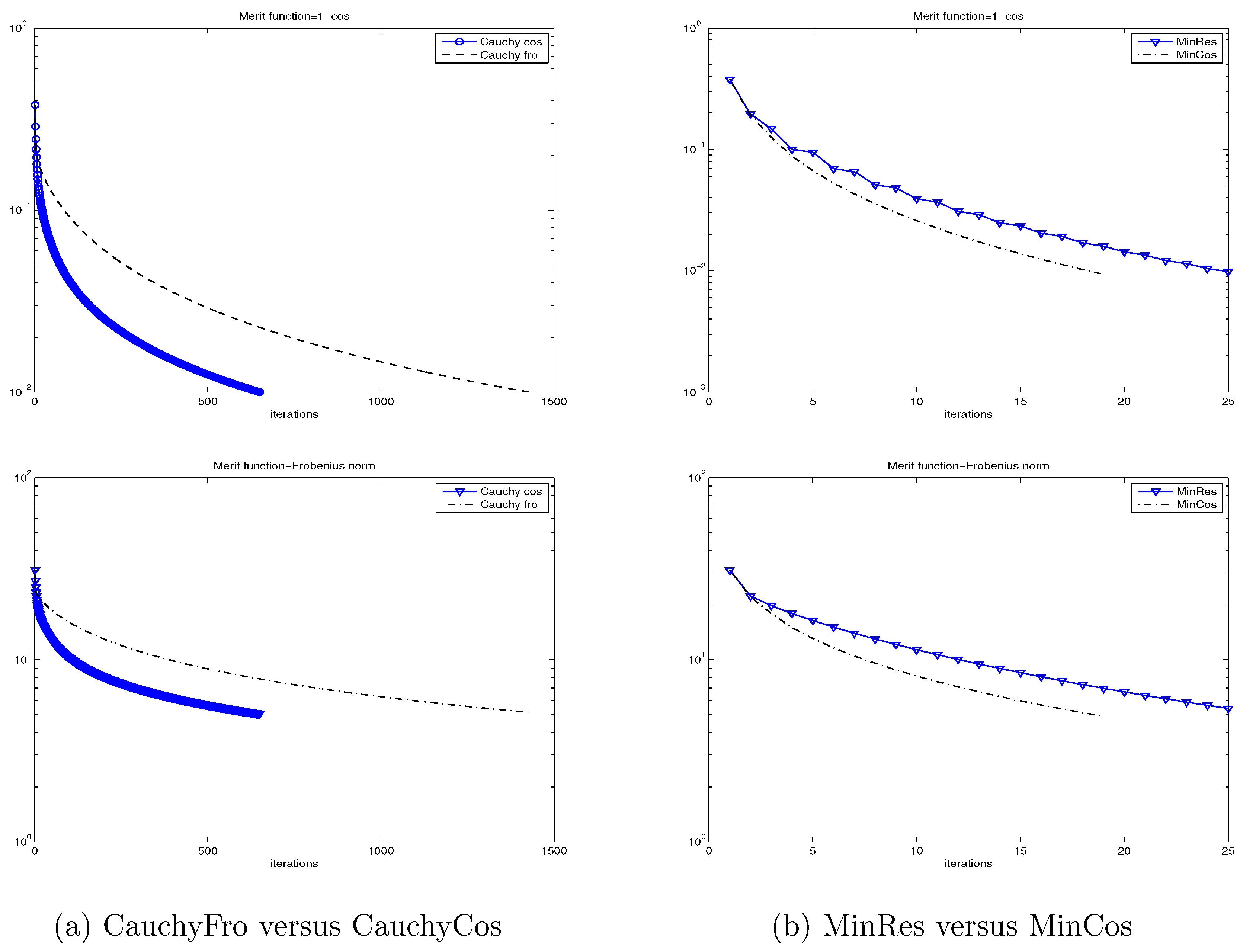
In Figure 1, we show the (semilog) convergence history for the four considered methods and for both merit functions: $F(X)$ and $\Phi (X)$, when applied to the Wathen matrix for $n=20$ and $ϵ=0.01$. Once again, we can observe that CauchyFro and CauchyCos are not competitive with MinRes and MinCos, and that MinCos outperforms MinRes. Moreover, we observe in this case that the function $F(X)$ is a better merit function than $\Phi (X)$ in the sense that it indicates with fewer iterations that a given iterate is sufficiently close to the inverse matrix. The same good behavior of the merit function $F(X)$ has been observed in all our experiments.

Based on these preliminary results, we will only report the behavior of MinRes and MinCos for the forthcoming numerical experiments.

3.2. Sparse Approximation to the Inverse

We now build sparse approximations by applying the dropping strategy, described in Section 2.5, which is based on a threshold tolerance with a limited fill-in ($lfil$) on the matrix $Z^{(k+1)}$, at each iteration, right before the scaling step to guarantee that the iterate $X^{(k+1)}\in S\cap T$. We define $thr$ as the percentage of coefficients less than the maximum value of the modulus of all the coefficients in a column. To be precise, for each i-th column, we select at most $lfil$ off-diagonal coefficients among the ones that are larger in magnitude than $thr\times \parallel {(Z^{(k+1)})}_i{\parallel }_{\infty }$, where ${(Z^{(k+1)})}_i$ represents the i-th column of $Z^{(k+1)}$. Once the sparsity has been imposed at each column and a sparse matrix is obtained, say $sp(Z^{(k+1)})$, we guarantee symmetry by setting $Z^{(k+1)}=(sp(Z^{(k+1)})+sp{(Z^{(k+1)})}^T)/2$.

We have implemented the relatively simple dropping strategy, described above, for both MinRes and MinCos to make a first validation of the new method. Of course, we could use a more sophisticated dropping procedure for both methods as one can find in [6]. The current numerical comparison is preliminary and indicates the potential of MinCos versus MinRes. We begin by comparing both methods when we apply the numerical described dropping strategy on the Matrix Market matrices.

Table 3. Performance of MinRes and MinCos when applied to the Matrix Market matrices nos1, nos2, nos5, and nos6, for $ϵ=0.01$, $thr=0.01$, and different values of $lfil$.

Matrix	Method	$\mathit{\kappa }\mathbf{\left(}{\mathit{X}}^{\mathbf{\left(}\mathit{k}\mathbf{\right)}}\mathit{A}\mathbf{\right)}$$/\mathit{\kappa }\mathbf{\left(}\mathit{A}\mathbf{\right)}$	$\mathbf{[}{\mathit{\lambda }}_{\mathit{min}}\mathbf{,}{\mathit{\lambda }}_{\mathit{max}}\mathbf{]}$ of $\mathbf{\left(}{\mathit{X}}^{\mathbf{\left(}\mathit{k}\mathbf{\right)}}\mathit{A}\mathbf{\right)}$	Iter	% Fill-in
nos1 ($lfil=10$)	MinCos	0.0835	[2.44 × 10−6,2.3272]	20	3.71
nos1($lfil=10$)	MinRes		[−98.66,5.40]
nos6 ($lfil=10$)	MinCos	0.4218	[5.07 × 10−6,3.1039]	20	0.45
nos6 ($lfil=20$)	MinCos	0.2003	[8.51 × 10−6,3.0702]	20	0.82
nos6 ($lfil=10$)	MinRes		[−0.7351,2.6001]
nos6 ($lfil=20$)	MinRes		[−0.2256,2.2467]
nos5 ($lfil=5$)	MinCos	0.068	[0.002,1.36]	10	1.18
nos5 ($lfil=10$)	MinCos	0.0755	[00.0024,1.3103]	10	2.47
nos5 ($lfil=5$)	MinRes		[−20.31,2.16]
nos5 ($lfil=10$)	MinRes	0.1669	[0.0021,1.7868]	10	2.36
nos2 ($lfil=5$)	MinCos	0.1289	[5.2 × 10−9,2.73]	10	0.52
nos2 ($lfil=10$)	MinCos	0.0891	[7.95 × 10−9,2.2873]	10	0.80
nos2 ($lfil=20$)	MinCos	0.0700	[9.7 × 10−9,1.9718]	10	1.14
nos2 ($lfil=5$)	MinRes		[−0.3326,2.4869]
nos2 ($lfil=10$)	MinRes	0.0970	[4.21 × 10−9,1.5414]	10	0.93
nos2 ($lfil=20$)	MinRes	0.0861	[4.21 × 10−9,1.1638]	10	1.14

shows the performance of MinRes and MinCos when applied to the matrices nos1, nos2, nos5, and nos6, for $ϵ=0.01$, $thr=0.01$, and several values of $lfil$. We report the iteration k (Iter) at which the method was stopped, the interval $[{\lambda }_{min},{\lambda }_{max}]$ of $(X^{(k)}A)$, the quotient $\kappa (X^{(k)}A)$/$\kappa (A)$, and the percentage of fill-in (% fill-in) at the final matrix $X^{(k)}$. 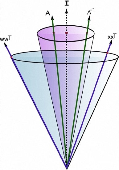We observe that, when imposing the dropping strategy to obtain sparsity, MinRes fails to produce an acceptable preconditioner. Indeed, as it has been already observed (see [6,15]) quite frequently that MinRes produces an indefinite approximation to the inverse of a sparse matrix in the $PSD$ cone. We also observe that, in all cases, the MinCos method produces a sparse symmetric and positive definite preconditioner with relatively few iterations and a low level of fill-in. Moreover, with the exception of the matrix nos6, the MinCos method produces a preconditioned matrix $(X^{(k)}A)$ whose condition number is reduced by a factor of approximately 10 with respect to the condition number of A. In some cases, MinRes was capable of producing a sparse symmetric and positive definite preconditioner, but in those cases, the MinCos produced a better preconditioner in the sense that it exhibits a better reduction of the condition number, and also a better eigenvalues distribution. Based on these results, for the remaining experiments, we only report the behavior of the MinCos Algorithm.

Table 4. Performance of MinCos applied to the Wathen matrix for different values of n and a maximum of 20 iterations, when $ϵ=0.01$, $thr=0.04$, and $lfil=20$.

Matrix A	Size (n × n)	$\mathit{\kappa }\mathbf{\left(}{\mathit{X}}^{\mathbf{\left(}\mathit{k}\mathbf{\right)}}\mathit{A}\mathbf{\right)}$$/\mathit{\kappa }\mathbf{\left(}\mathit{A}\mathbf{\right)}$	$\mathbf{[}{\mathit{\lambda }}_{\mathit{min}}\mathbf{,}{\mathit{\lambda }}_{\mathit{max}}\mathbf{]}$ of $\mathbf{\left(}{\mathit{X}}^{\mathbf{\left(}\mathit{k}\mathbf{\right)}}\mathit{A}\mathbf{\right)}$	Iter	% Fil-in
wathen (30)	n=2821	0.0447	$[0.0109,1.3889]$	20	0.73
wathen (50)	n=7701	0.0461	$[0.0366,1.4012]$	20	0.27
wathen (70)	n=14981	0.0457	$[0.0086,1.3894]$	20	0.14
wathen (100)	n=30401	0.0467	$[0.0289,1.4121]$	20	6.8436 × 10−2

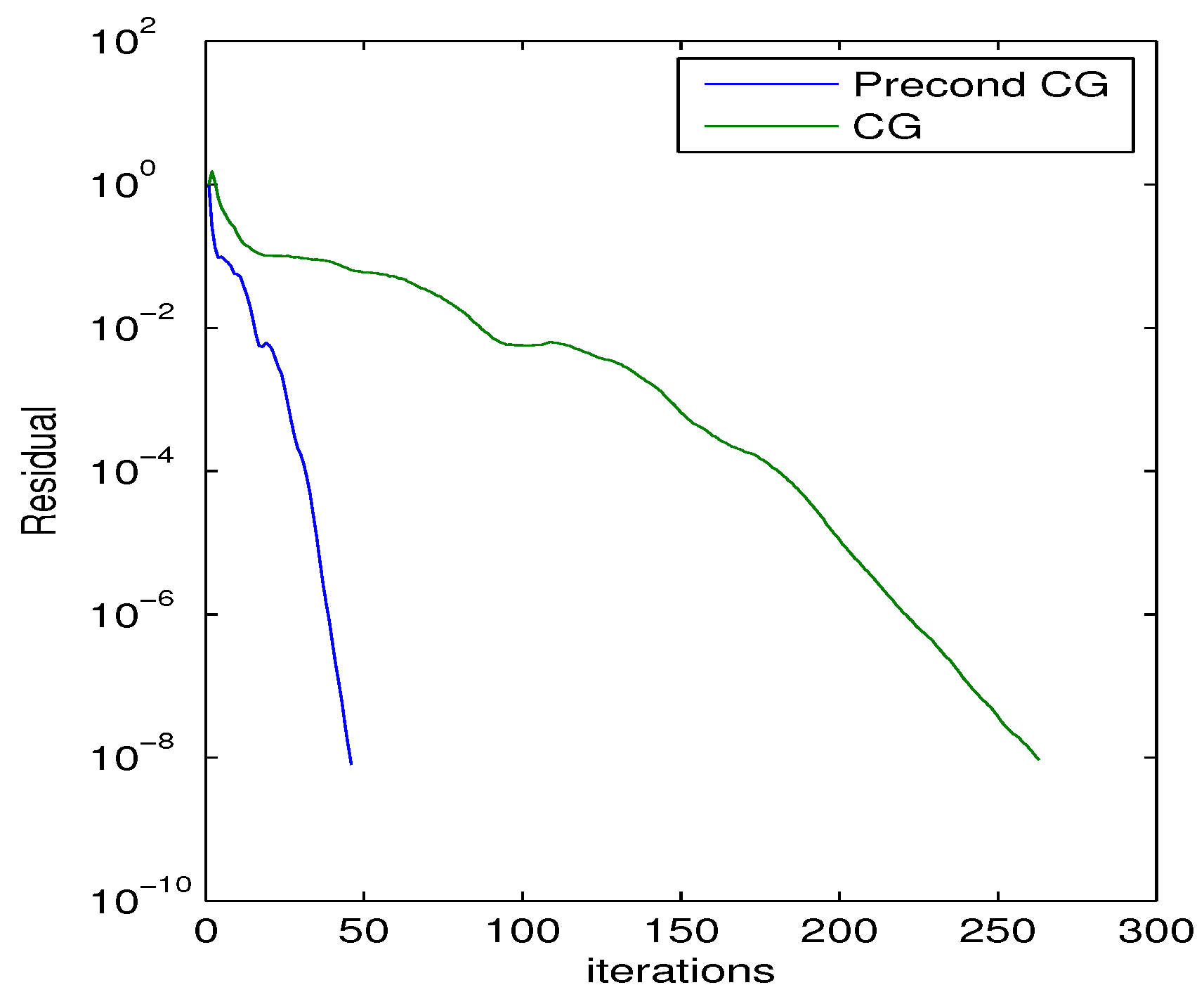
shows the performance of the MinCos Algorithm when applied to the Wathen matrix for different values of n and a maximum of 20 iterations. For this numerical experiment, we fix $ϵ=0.01$, $thr=0.04$, and $lfil=20$. For the particular case of the Wathen matrix when $n=50$, we show in Figure 2 that the (semilog) convergence history of the norm of the residual when solving a linear system with a random right-hand side vector, using the Conjugate Gradient (CG) method without preconditioning, and also using the preconditioner generated by the MinCos Algorithm after 20 iterations, fixing $ϵ=0.01$, $thr=0.04$, and $lfil=20$. 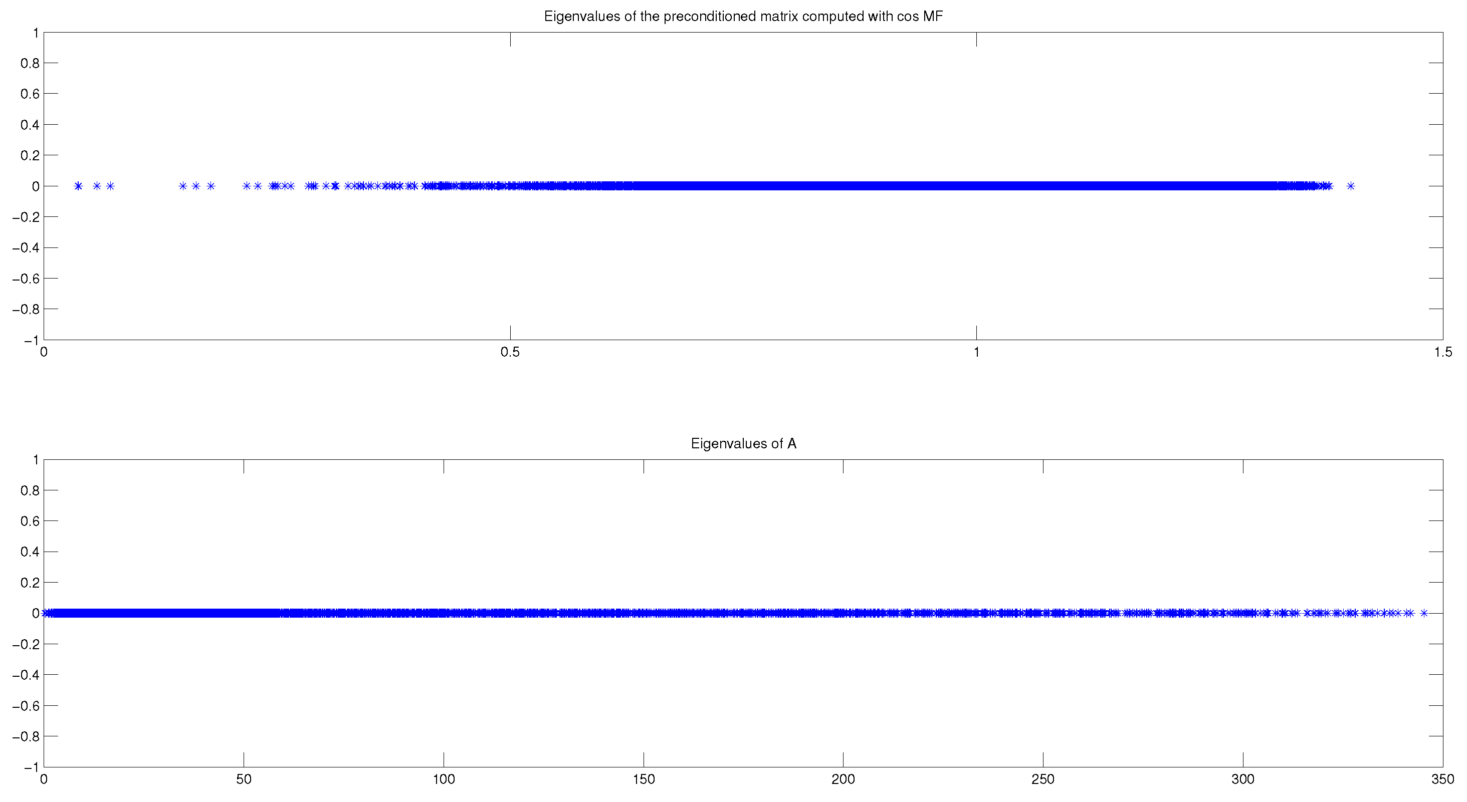We also report in Figure 3 the eigenvalues distribution of A and of $X^{(k)}A$, at $k=20$, for the same experiment with the Wathen matrix and $n=50$. Notice that the eigenvalues of A are distributed in the interval $[0,350]$, whereas the eigenvalues of $X^{(k)}A$ are located in the interval $[0.03,1.4]$ (see Table 4). Even better, we can observe that most of the eigenvalues are in the interval $[0.3,1.4]$, and very few of them are in the interval $[0.03,0.3]$, which clearly accounts for the good behavior of the preconditioned CG method (see Figure 2).

Table 5. Performance of MinCos applied to the Poisson 2D matrix, for different values of n and a maximum of 20 iterations, when $ϵ=0.01$, $thr=0.04$, and $lfil=40$.

Matrix A	Size n × n	$\mathit{\kappa }\mathbf{\left(}{\mathit{X}}^{\mathbf{\left(}\mathit{k}\mathbf{\right)}}\mathit{A}\mathbf{\right)}$$/\mathit{\kappa }\mathbf{\left(}\mathit{A}\mathbf{\right)}$	$\mathbf{[}{\mathit{\lambda }}_{\mathit{min}}\mathbf{,}{\mathit{\lambda }}_{\mathit{max}}\mathbf{]}$ of $\mathbf{\left(}{\mathit{X}}^{\mathbf{\left(}\mathit{k}\mathbf{\right)}}\mathit{A}\mathbf{\right)}$	Iter	% Fil-in
Poisson 2D (50)	n = 2500	0.1361	$[0.0138,1.2961]$	6	1.65
Poisson 2D (100)	n = 10000	0.1249	$[0.0039,1.1452]$	7	0.41
Poisson 2D (150)	n = 22500	0.1248	$[0.0017,1.1459]$	7	0.18
Poisson 2D (200)	n = 40000	0.1246	[9.78 × 10−4,1.1484]	7	0.10

,

Table 6. Performance of MinCos applied to the Poisson 3D matrix, for different values of n and a maximum of 20 iterations, when $ϵ=0.01$, $thr=0.01$, and $lfil=40$.

Matrix A	Size n × n	$\mathit{\kappa }\mathbf{\left(}{\mathit{X}}^{\mathbf{\left(}\mathit{k}\mathbf{\right)}}\mathit{A}\mathbf{\right)}$$/\mathit{\kappa }\mathbf{\left(}\mathit{A}\mathbf{\right)}$	$\mathbf{[}{\mathit{\lambda }}_{\mathit{min}}\mathbf{,}{\mathit{\lambda }}_{\mathit{max}}\mathbf{]}$ of $\mathbf{\left(}{\mathit{X}}^{\mathbf{\left(}\mathit{k}\mathbf{\right)}}\mathit{A}\mathbf{\right)}$	Iter	% Fil-in
Poisson 3D (10)	n=1000	0.3393	$[0.1161,1.4410]$	2	2.09
Poisson 3D(15)	n=3375	0.3357	$[0.0561,1.4639]$	2	0.66

and

Table 7. Performance of MinCos applied to the Lehmer matrix, for different values of n and a maximum of 40 iterations, when $ϵ=0.01$, $thr=0.06$, and $lfil=100$.

Matrix A	$\mathit{\kappa }\mathbf{\left(}{\mathit{X}}^{\mathbf{\left(}\mathit{k}\mathbf{\right)}}\mathit{A}\mathbf{\right)}$$/\mathit{\kappa }\mathbf{\left(}\mathit{A}\mathbf{\right)}$	$\mathbf{[}{\mathit{\lambda }}_{\mathit{min}}\mathbf{,}{\mathit{\lambda }}_{\mathit{max}}\mathbf{]}$ of $\mathbf{\left(}{\mathit{X}}^{\mathbf{\left(}\mathit{k}\mathbf{\right)}}\mathit{A}\mathbf{\right)}$	Iter	% Fil-in
Lehmer (100)	0.0150	$[0.0223,3.4270]$	40	37.04
Lehmer (200)	0.0180	$[0.0069,5.0768]$	40	38.34

show the performance of the MinCos Algorithm when applied to the Poisson 2D, the Poisson 3D, and the Lehmer matrices, respectively, for different values of n, and different values of the maximum number of iterations, ϵ, $thr$, and $lfil$. We can observe that, for the Poisson 2D and 3D matrices, the MinCos Algorithm produces a sparse symmetric and positive definite preconditioner with very few iterations, a low level of fill-in, and a significant reduction of the condition number.

For the Lehmer matrix, which is one of the most difficult considered matrices, we observe in Table 7 that the MinCos Algorithm produces a symmetric and positive definite preconditioner with a significant reduction of the condition number, but after 40 iterations and fixing $lfil=100$, for which the preconditioner accepts a high level of fill-in. If we impose a low level of fill-in, by reducing the value of $lfil$, MinCos still produces a symmetric and positive definite matrix, but the reduction of the condition number is not significant.

We close this section mentioning that both methods (MinCos and MinRes) produce sparse approximations to the inverse with comparable sparsity as shown in Table 3 (last column). Notice also that MinCos produces a sequence $X^{(k)}$ such that the eigenvalues of $X^{(k)}A$ are strictly positive at convergence, which, in turn, implies that the matrices $X^{(k)}$ are invertible after a sufficiently large k. This important property cannot be satisfied by MinRes.

4. Conclusions

We have introduced and analyzed two gradient-type optimization schemes to build sparse inverse preconditioners for symmetric positive definite matrices. For that, we have proposed the novel objective function $F(X)=1-cos(XA,I)$, which is invariant under positive scaling and has some special properties that are clearly related to the geometry of the $PSD$ cone. One of the new schemes, the CauchyCos Algorithm, is closely related to the classical steepest descent method, and as a consequence, it shows in most cases a very slow convergence. The second new scheme, denoted as the MinCos Algorithm, shows a much faster performance and competes favorably with well-known methods. Based on our numerical results, by choosing properly the numerical dropping parameters, the MinCos Algorithm produces a sparse inverse preconditioner in the $PSD$ cone for which a significant reduction of the condition number is observed, while keeping a low level of fill-in.