An Adaptive WENO Collocation Method for Differential Equations with Random Coefficients

Abstract

The stochastic collocation method for solving differential equations with random inputs has gained lots of popularity in many applications, since such a scheme exhibits exponential convergence with smooth solutions in the random space. However, in some circumstance the solutions do not fulfill the smoothness requirement; thus a direct application of the method will cause poor performance and slow convergence rate due to the well known Gibbs phenomenon. To address the issue, we propose an adaptive high-order multi-element stochastic collocation scheme by incorporating a WENO (Weighted Essentially non-oscillatory) interpolation procedure and an adaptive mesh refinement (AMR) strategy. The proposed multi-element stochastic collocation scheme requires only repetitive runs of an existing deterministic solver at each interpolation point, similar to the Monte Carlo method. Furthermore, the scheme takes advantage of robustness and the high-order nature of the WENO interpolation procedure, and efficacy and efficiency of the AMR strategy. When the proposed scheme is applied to stochastic problems with non-smooth solutions, the Gibbs phenomenon is mitigated by the WENO methodology in the random space, and the errors around discontinuities in the stochastic space are significantly reduced by the AMR strategy. The numerical experiments for some benchmark stochastic problems, such as the Kraichnan-Orszag problem and Burgers’ equation with random initial conditions, demonstrate the reliability, efficiency and efficacy of the proposed scheme.

1. Introduction

Problems subject to uncertainty arise in many engineering [1,2], environmental and biological applications. Such uncertainty is mainly due to a lack of knowledge about the true value of model parameters or the random nature of the quantity of interest being studied. Uncertainty quantification (UQ) for practical problems has been drawing growing interest in recent years, in particular in developing numerical methods for stochastic computations. Due to the computational cost of high-fidelity models for complex systems, many researchers are investigating more efficient stochastic algorithms than the classic Monte Carlo (MC) method. One of the popular stochastic methodologies is generalized polynomial chaos (gPC) [3], which is an extension of the standard polynomial chaos method [4]. In addition, advanced gPC algorithms for high-dimensional stochastic problems have been developed [5,6,7,8,9,10,11,12,13,14,15].

The performance and convergence of gPC depends on the smoothness of the function in the random parameter space. gPC will converge quickly for smooth functioning in random parameter space. However, the performance and convergence will deteriorate when the function has low regularity, particularly with discontinuities in the random parameter space. In such cases, Gibbs-type phenomenon will be observed in gPC approximation, which causes the slow convergence. To alleviate such a challenging issue, multi-element gPC methods [16,17] and multi-element stochastic collocation methods [18,19] were developed to decompose the random space into sub-domains, then employ a gPC expansion in each element. The challenge of the standard multi-element gPC or multi-element stochastic collocation method is to detect the discontinuities in high-dimensional random space and the computational cost. It requires the users to resolve the stochastic problem in each of the random element. A few recent works on the development of efficient stochastic algorithms for handling discontinuities also exist [20,21,22,23,24,25,26].

In this paper, we propose an adaptive high-order multi-element stochastic collocation method in conjunction with Weighted Essentially non-oscillatory (WENO) reconstruction methodology and adaptive mesh refinement (AMR) strategy to address the challenging issue regarding standard multi-element approaches for solving stochastic differential equations with discontinuities in the random space. The proposed method consists of two important components. (1) Adaptive stochastic domain decomposition framework: it is known that solution in the random space may exhibit local complex structures such as discontinuities; hence, we employ a stochastic domain decomposition framework based on the idea that in the smooth region a multi-element stochastic collocation scheme is used in order to take advantage of its low computational cost and fast convergence, while an AMR WENO scheme on a local tensor-product grid is used in the region with complex discontinuous solution structures; (2) High-order WENO interpolation scheme in random space: it is a grand challenge to detect the discontinuities in high-dimensional random space. However, by employing the WENO scheme, there is no need to know the location of the discontinuities exactly. High-order WENO interpolation scheme in random space can provide essentially non-oscillatory solutions across the discontinuities, which is particular suitable for stochastic problems with complex discontinuity structure; (3) AMR strategy in random space [27]: Even though the AMR WENO scheme has been developed in different settings in the literature, such as an AMR WENO scheme for solving hyperbolic conservation laws [27], it has not been investigated in the uncertainty quantification context. By employing AMR strategy, we can identify the regions that contain discontinuities in random space and only apply the high-order WENO interpolation scheme in such regions. In this paper, we will show the efficiency and efficacy of the proposed scheme for solving stochastic problems with complex solution structure including discontinuities.

This paper is organized as follows: in the next section, the mathematical formulation of the proposed stochastic domain decomposition framework, high-order WENO interpolation, and AMR strategy in random space is introduced. In Section 3, the numerical examples are given. Finally, concluding remarks are provided in Section 4.

2. Formulation

In this section, we formulate the adaptive AMR WENO-based multi-element stochastic collocation scheme for solving differential equations with random inputs. We start with a review of the multi-element stochastic collocation method, the high-order WENO interpolation methodology for non-smooth problems, which has been widely used in many applications. In the second part, an ARM strategy in conjunction with the WENO interpolation is formulated in order to take advantage of both numerical ingredients.

2.1. Multi-Element Stochastic Collocation Method (ME-SCM)

The ME-SCM introduced in [19] decomposes the random space Γ into non-overlapping elements and then employs the stochastic collocation method on each element. This will provide the approximation of local moment statistics in each element. We can assemble such local moment statistics in each element to obtain the global statistics. To improve the efficiency of the proposed ME-SCM, both the high-order WENO interpolation scheme and AMR strategy will be employed, which will be discussed in the following subsections.

In particular, we discretize the parametric space Γ into a nonoverlapping mesh of open hypercubes. We denote ${\left\{B^i\right\}}_{i=1}^{N_e}$ to be a finite collection of open subsets of Γ such that ${\bigcup }_{i=1}^{N_e}\overline{B^i}=\mathsf{\Gamma }$ and $B^i\bigcap B^j=\varnothing$ whenever $i\ne j$. For illustrative purposes, we let $B^i$ be hypercubes. These sets consists of the elements of a mesh on the random space Γ and $N_e$ denotes the number of elements. In the prescribed mesh, a set of collocation points ${\left\{{\mathbf{y}}_{i,q}\right\}}_{q=1}^s$ is prescribed in each element $B^i$. Here, s refers to the number of collocation points. The collocation points are selected so that they coincide with the points of an cubature rule on $B^i$ with integration weights ${\left\{w_{i,q}\right\}}_{q=1}^s$. In particular, we employ full tensor products of Gauss quadrature points as the collocation points.

At each of the collocation points ${\left\{{\mathbf{y}}_{i,q}\right\}}_{q=1}^s$, we obtain the numerical solution $u_k(\mathbf{x},{\mathbf{y}}_{i,q})$ of the corresponding deterministic problem,

$$\mathbb{L}(\mathbf{x},{\mathbf{y}}_{i,q};u_k(\mathbf{x},{\mathbf{y}}_{i,q}))=f(\mathbf{x},{\mathbf{y}}_{i,q}),\mathbf{x}\in D,\mathbb{B}(\mathbf{x},u_k(\mathbf{x},{\mathbf{y}}_{i,q}))=g\left(\mathbf{x}\right),\mathbf{x}\in \partial D$$

(1)

The fully discrete approximation ${\mathbb{I}}_{B^i}{u}_k(\mathbf{x},\mathbf{y})$ based on the tensor product Lagrangian interpolant can be written as:

$${\mathbb{I}}_{B^i}{u}_k(\mathbf{x},\mathbf{y})\equiv L_{B^i}^p{u}_k(\mathbf{x},\mathbf{y})=\sum _{q=1}^s{u}_k(\mathbf{x},{\mathbf{y}}_{i,q})l_q^i\left(\mathbf{y}\right)$$

(2)

where p determines the degree of the interpolant in each dimension. $l_j^i\left(\mathbf{y}\right)$ is the Lagrange polynomial with respect to the quadrature point ${\mathbf{y}}_{i,q}$.

The global approximant is defined as,

$$\tilde{u}(\mathbf{x},\mathbf{y})=\sum _{i=1}^{N_e}{\mathbb{I}}_{B^i}{u}_k(\mathbf{x},\mathbf{y}){{\rm Y}}_{\{\mathbf{y}\in B^i\}}\forall \mathbf{x}\in \overline{D},\forall \mathbf{y}\in \mathsf{\Gamma }$$

(3)

where ${{\rm Y}}_{\{\mathbf{y}\in B^i\}}$ is the characteristic function of set $B^i$.

The corresponding probability density function in each element is defined as,

$${\eta }^i\left(\mathbf{y}\right)=\frac{\rho \left(\mathbf{y}\right)}{{\int }_{B^i}\rho \left(\mathbf{y}\right)d\mathbf{y}}$$

(4)

where $\rho \left(\mathbf{y}\right)={\prod }_{j=1}^N{\rho }_j\left(y_j\right)$. The local mean of a function u in an element i is given by,

$${\mathbb{E}}^i[u(\mathbf{x},\mathbf{y}]={\int }_{B^i}u(\mathbf{x},\mathbf{y}){\eta }^i\left(\mathbf{y}\right)d\mathbf{y}$$

(5)

The approximation of local mean of $\tilde{u}$ using the cubature rule over each element can be computed as,

$${\tilde{\mathbb{E}}}^i\left[\tilde{u}\right]\left(\mathbf{x}\right)=\sum _{q=1}^s{u}_k(\mathbf{x},{\mathbf{y}}_{i,q})w_{i,q}\approx {\mathbb{E}}^i\left[\tilde{u}\right]\left(\mathbf{x}\right)$$

(6)

where ${\tilde{\mathbb{E}}}^i$ is the expected value approximation operator using numerical quadrature rule. The approximate global mean can be obtained from the local mean as:

$$\tilde{\mathbb{E}}\left[\tilde{u}\right]\left(\mathbf{x}\right)=\sum _{i=1}^{N_e}{\tilde{\mathbb{E}}}^i\left[\tilde{u}\right]\left(\mathbf{x}\right)P(\mathbf{Y}\left(\omega \right)\in B^i)\approx \mathbb{E}\left[\tilde{u}\right]\left(\mathbf{x}\right)$$

(7)

Other statistics can be obtained by a similar procedure.

2.2. High-Order WENO Interpolation in Random Space

The widely recognized WENO interpolation method is known to be able to effectively resolve non-smooth data. By carefully assigning weights to each stencil candidate, the WENO interpolation attains high order accuracy in the smooth region while avoiding oscillations in regions with singularities (see [28] for a detailed review on the recent development and applications).

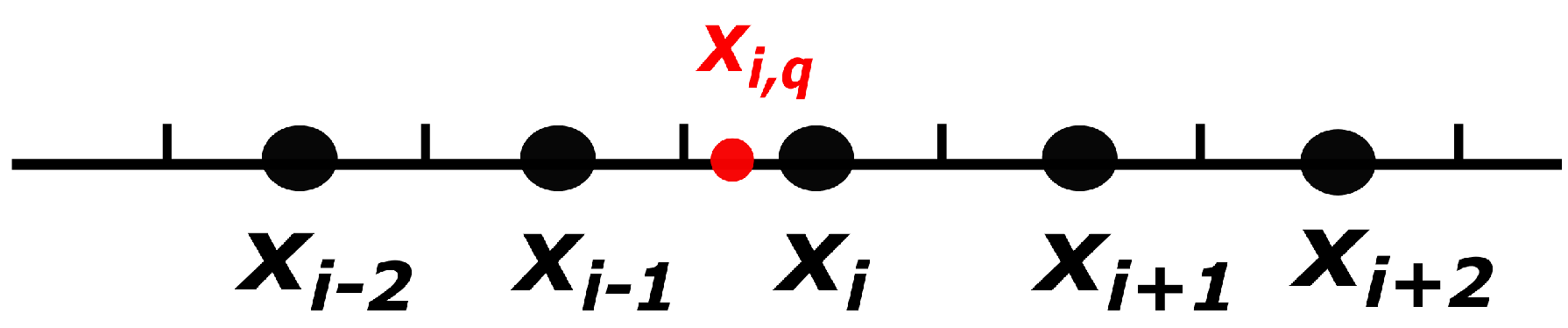
2.2.1. One-Dimensional Case

We start with the simple one-dimensional case. The extension to high-dimensional problems can be established by a tensor product construction and will be discussed later. Consider the following problem: given a set of point values $u_i$ on a uniform mesh $x_i$ in a bound domain, $i=1,\dots ,N$ with a mesh size $\Delta x=x_{i+1}-x_i$, we need to interpolate a local polynomial approximating the original function $u\left(x\right)$ with high order accuracy and free of oscillations. Such a local polynomial $u_i^h\left(x\right)$ can be reconstructed as follows.

Assume that we would like to obtain a fifth order approximation from five point values $u_{i-2}$, $u_{i-1}$, $u_i,$ $u_{i+1}$, $u_{i+2}$. Rather than directly reconstructing a polynomial on the interval $[x_{i-1/2},x_{x+1/2}]$, we first interpolate the values at five local quadrature points $x_{i,q}$, $q=1,\dots ,5$, see Figure 1, then obtain the polynomial from the values at these points. Such an idea has been used to develop the WENO limiter for discontinuous Galerkin (DG) schemes [29]. First, note that for each point $x_{i,q}$, we have three interpolation values

$$\begin{array}{cc}\hfill v_{i,q}^{\left(0\right)}& =c_{0,q}^{\left(0\right)}{u}_{i-2}+c_{1,q}^{\left(0\right)}{u}_{i-1}+c_{2,q}^{\left(0\right)}{u}_i\hfill \\ \hfill v_{i,q}^{\left(1\right)}& =c_{0,q}^{\left(1\right)}{u}_{i-1}+c_{1,q}^{\left(1\right)}{u}_i+c_{2,q}^{\left(1\right)}{u}_{i+1}\hfill \\ \hfill v_{i,q}^{\left(2\right)}& =c_{0,q}^{\left(2\right)}{u}_i+c_{1,q}^{\left(2\right)}{u}_{i+1}+c_{2,q}^{\left(2\right)}{u}_{i+2}\hfill \end{array}$$

from three small stencils as third order approximations, and

$$v_{i,q}=c_{0,q}{u}_{i-2}+c_{1,q}{u}_{i-1}+c_{2,q}{u}_i+c_{3,q}{u}_{i+1}+c_{4,q}{u}_{i+1}+c_{5,q}{u}_{i+2}$$

from the large stencil as a fifth order approximation of the underlying function. We can also seek a set of linear weights $d_q^{\left(r\right)}$, $r=0,1,2,$ such that

$$v_{i,q}=v_{i,q}^{\left(0\right)}{d}_q^{\left(0\right)}+v_{i,q}^{\left(1\right)}{d}_q^{\left(1\right)}+v_{i,q}^{\left(2\right)}{d}_q^{\left(2\right)}$$

(8)

Note that a direct application of linear weights $d_q^{\left(r\right)}$ will lead to oscillations due to the famous Gibbs phenomenon. Instead, they are replaced by the nonlinear weights, which is known as the main idea of the WENO methodology. Denote three local polynomials of degree two on each small stencil by $p^{\left(r\right)}\left(x\right)$. Then, the smoothness indicators measuring the relative smoothness of each stencil are defined as:

$${\beta }^{\left(r\right)}=\sum _{l=1}^2{\int }_{x_{i-\frac{1}{2}}}^{x_{i+\frac{1}{2}}}\Delta x^{2l-1}\left(\frac{{\partial }^l{p}^{\left(r\right)}\left(x\right)}{{\partial }^{l}x}\right)dx$$

In particular, it gives

$$\begin{array}{cc}\hfill {\beta }^{\left(0\right)}=& \frac{13}{12}{(u_{i-2}-2u_{i-1}+u_i)}^2+\frac{1}{4}{(u_{i-2}-4u_{i-1}+3u_i)}^2\hfill \\ \hfill {\beta }^{\left(1\right)}=& \frac{13}{12}{(u_{i-1}-2u_i+u_{i+1})}^2+\frac{1}{4}{(u_{i-1}-u_{i-1})}^2\hfill \\ \hfill {\beta }^{\left(2\right)}=& \frac{13}{12}{(u_i-2u_{i+1}+u_{i+2})}^2+\frac{1}{4}{(3u_i-4u_{i+1}+u_{i+2})}^2\hfill \end{array}$$

Then, the nonlinear weights are defined accordingly as:

$$w_q^{\left(r\right)}=\frac{{\alpha }^{{\left(r\right)}_q}}{{\sum }_{s=0}^2{\alpha }_q^{\left(r\right)}},{\alpha }_q^{\left(r\right)}=\frac{d_q^{\left(r\right)}}{{(\epsilon +{\beta }^{\left(r\right)})}^2},r=0,1,2$$

where ε is chosen as a small number ${10}^{-6}$ in order to avoid zero denominator. Lastly, the interpolation values at quadrature nodes are obtained by applying the nonlinear weights, i.e.,

$${\tilde{v}}_{i,q}=v_{i,q}^{\left(0\right)}{w}_q^{\left(0\right)}+v_{i,q}^{\left(1\right)}{w}_q^{\left(1\right)}+v_{i,q}^{\left(2\right)}{w}_q^{\left(2\right)}$$

(9)

Based on the WENO interpolation values at the quadrature points ${\tilde{v}}_{i,q},$ $q=1,\dots ,5$, we are able to reconstruct a polynomial $\tilde{u}\left(x\right)$ of degree four. We remark that ${\tilde{v}}_{i,q},$ $q=1,\dots ,5$ share the same set of smoothness indicators, and the interpolation polynomial $\tilde{u}\left(x\right)$ automatically attains the desired essentially non-oscillatory properties.

If a cell is close to boundaries, then we need to apply a one-sided WENO interpolation procedure proposed in [30] to avoid oscillations. For brevity, we do not review the details but refer the readers to [30]. We also remark that, if only the first several moments such as mean or variance are of interest, the WENO reconstruction can be directly applied to compute such quantities to save computational cost. In particular, we only need to perform the WENO interpolation for several moments rather than the whole solution.

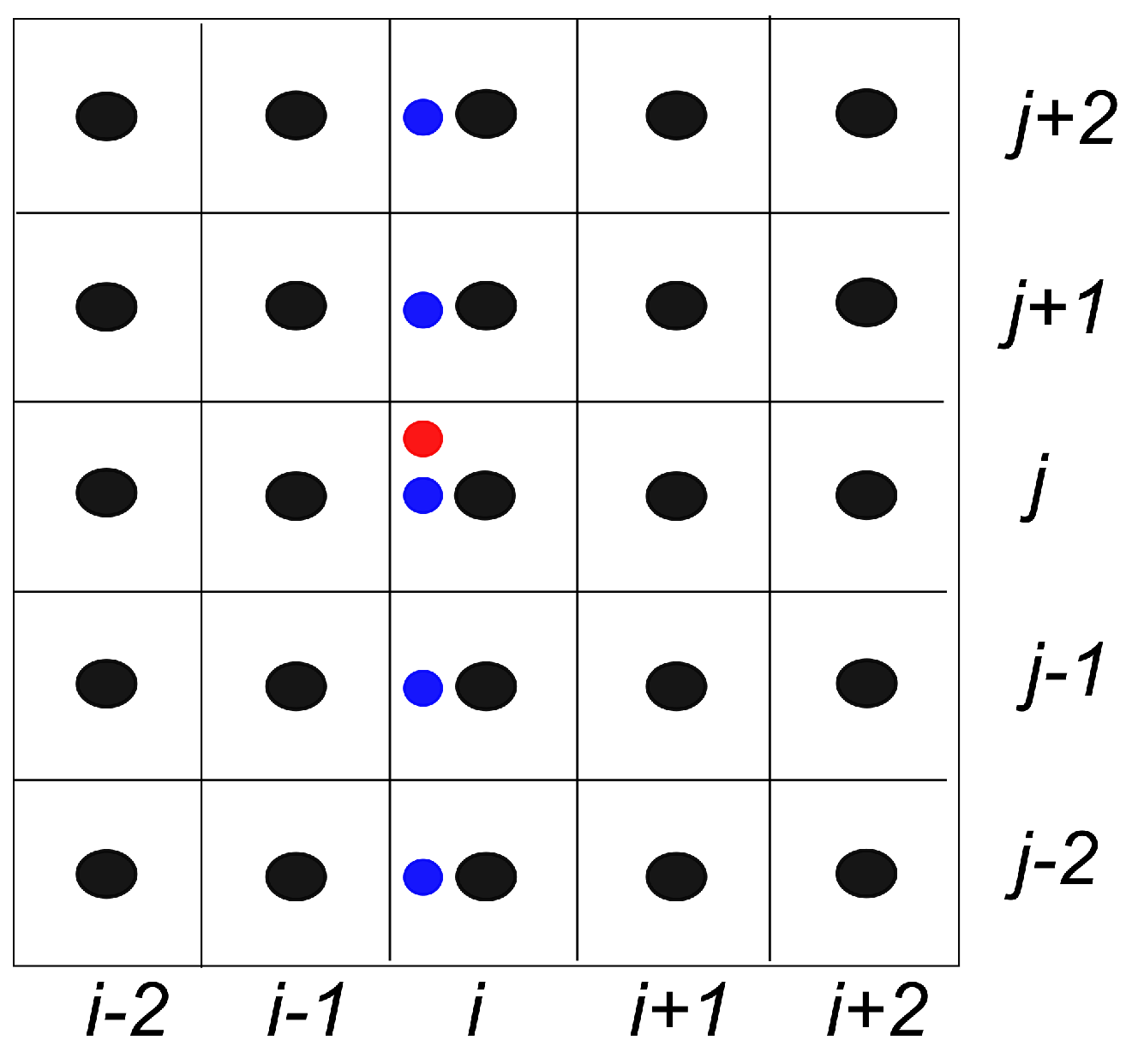
2.2.2. Two-Dimensional Extension

The extension of the WENO interpolation methodology to two-dimensional cases is based on a tensor product construction. Specifically, in order to obtain a fifth order approximation ${\tilde{u}}_{ij}\left(x\right)$, we need the stencil plotted in Figure 2. Similar to a one-dimensional case, we need to interpolate the point values ${\tilde{v}}_{ij,qg}$, $q,g=1,\dots ,5$ on the local cell $[x_{i-1/2},x_{i+1/2}]\times [y_{j-1/2},y_{j+1/2}]$, then reconstruct a polynomial of degree 4. The interpolation procedure is performed in a dimension-by-dimension fashion. To obtain the value ${\tilde{v}}_{ij,qg}$ (the red circle in Figure 2), we first apply the one-dimensional WENO interpolation in x-direction to get $v_{ir,q}$, $r=j-2,\dots ,j+2$ (the blue circles in Figure 2). Then, we can further apply the interpolation in y-direction. Once the values ${\tilde{v}}_{ij,qg}$ are obtained, the interpolating polynomial is constructed from ${\tilde{v}}_{ij,qg}$.

2.3. AMR Methodology in Random Space

The AMR methodology is known as an efficient numerical tool for solving problems with local complex solution structures, which has soared in popularity in many applications since the 1980s [31,32]. In this work, we consider a cluster based method to generate fine grids where the local mesh refinement is needed. It is also known that such a method is very suited for WENO interpolation on a tensor product grid. The AMR interpolation methodology has the following steps:

• Use a multi-resolution analysis to flag the regions of refinement interest (RRI): We compute the difference between the solution $u_{i,j}$ and the average of its four neighbors $b=\frac{1}{4}(u_{i+1,j}+u_{i-1,j}+u_{i,j+1},u_{i,j-1})$. If $|u_{i,j}-b|>ϵ\Delta x$, where ϵ is a user specified constant, then the point and its eight neighbors are marked as regions of refinement interest (RRI).
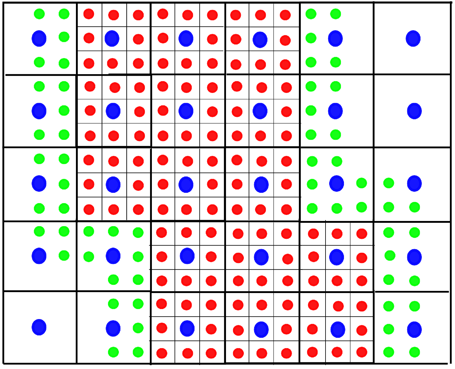
• Generate finer grids using the algorithm proposed in [33]: We generate some non-overlapping rectangular clusters that cover the RRI. In each cluster, the grid is refined with a ratio of three, i.e., $\Delta x_{l+1}=\Delta x_l/3$, where $\Delta x_l$ denotes the mesh size on the mesh level l (see Figure 3; two non-overlapping clusters are generated, and red circles denote point values on the fine grid).
• Repeat steps 1 and 2 until the maximal mesh level is attained.
• Generate the WENO interpolating polynomial by applying the algorithm reviewed in Section 2.2. We start from the clusters with the finest mesh level. The needed boundary values in the WENO interpolation procedure can be either obtained from the neighboring cluster with same mesh level or interpolated from coarser clusters. Again, the WENO interpolation should be used in order to avoid the oscillations (see Figure 3; the green circles are interpolated from the blue circles on a coarser cluster).

Note that the refinement ratio is set as three, since the solution on the coarse mesh level can be reused. Even though we only consider the two-dimensional case, the algorithm in [33] can be applied to problem in arbitrary dimension. Further, the rectangular clusters may contain some nodes are not RRI, however, the cutoff ratio is set as $0.7$ meaning that at least $70\%$ nodes included in the clusters are RRI.

Lastly, we remark that the use of tensor product grid seems less efficient than the sparse grid for high-dimensional problems. However, one should note that for many real applications in UQ, such as discontinuous response, the solution may have local dense structures in the random space. An adaptive sparse-grid based stochastic collocation scheme such as the one proposed in [26] still needs sufficient nodes clustered in the region to adequately represent the solution structures. Hence, in such a scenario, the computation cost of the tensor product grid is comparable to that of the sparse grid. Another rationale of the tensor product grid is that it is quite complicated to implement a high order WENO interpolation on an adaptive sparse grid, which is highly non-uniform. We leave the investigation of the WENO interpolation in conjunction with a sparse grid to the future work.

3. Numerical Results

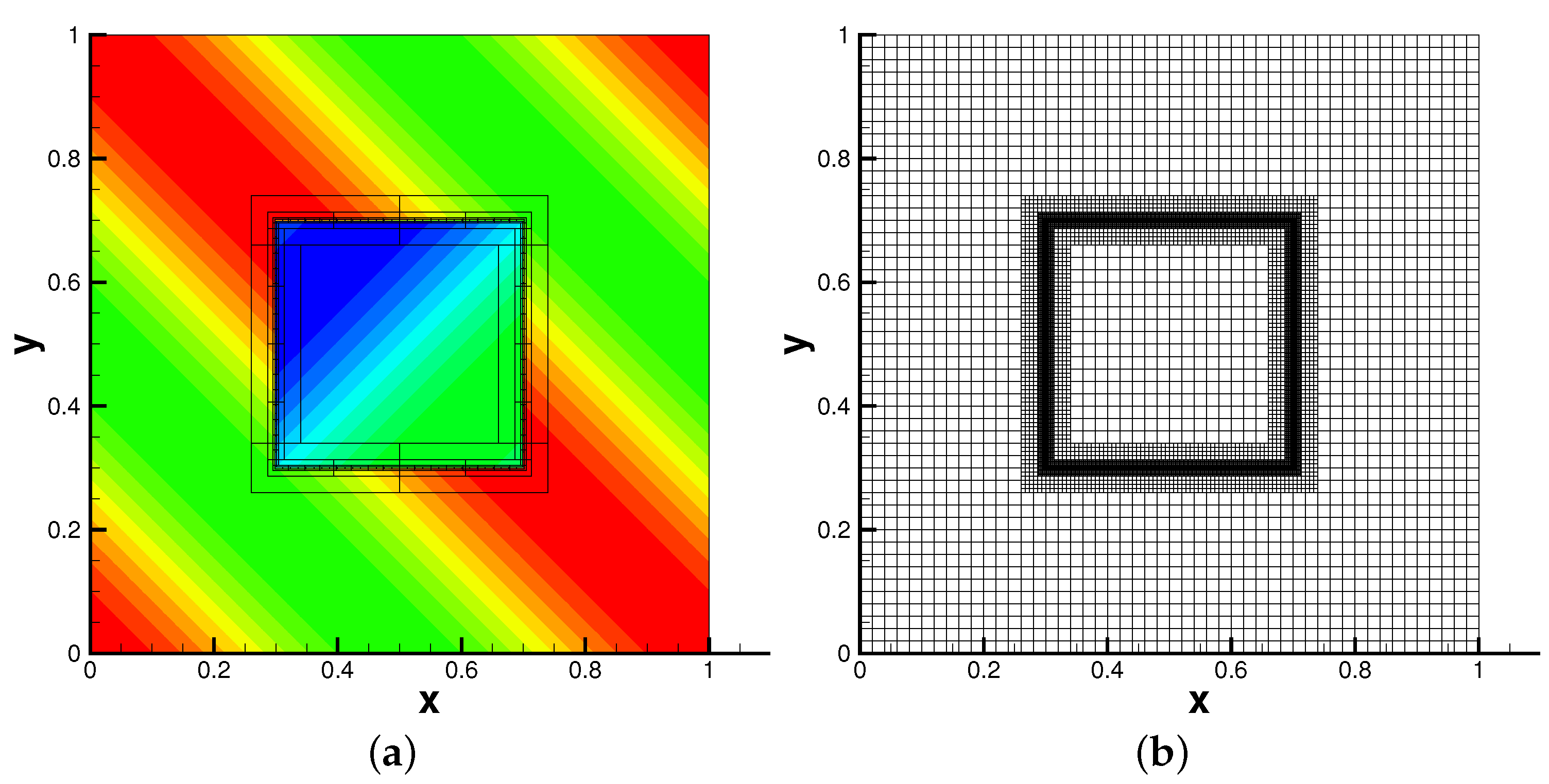
3.1. Approximation Investigation for Non-Smooth Functions

We first assess the approximation properties of the proposed AMR WENO stochastic collocation scheme. Below, we consider two functions with singularities in domain ${[0,1]}^2$:

$$f_1(x,y)=\frac{1}{|0.3-x^2-y^2|+0.1}$$

$${\displaystyle f_2(x,y)=\left\{\begin{array}{cc}sin\left(2\pi \right(x-y\left)\right)\hfill & (x,y)\in {[0.3,0.7]}^2\hfill \\ 2+cos\left(2\pi \right(x+y\left)\right)\hfill & \mathrm{otherwise}\hfill \end{array}\right.}$$

Note that $f_1$ has discontinuous derivative on the circle $x^2+y^2=0.3$ and $f_2$ is discontinuous with a line singularity parallel to the grid line. We start with the a tensor-product mesh $50\times 50$ and local mesh refinement is performed based on the multi-resolution analysis. The maximum mesh level is set as 4 and 5 for $f_1$ and $f_2$, respectively. In

Table 1. Approximation investigation of $f_1$. The error of variance (var. err.) and maximum error (max. err.) in 1000 randomly sampled points.

Mesh Level	$ϵ=10$			$ϵ=1$			$ϵ=0.1$
	points	var. err.	max. err.	points	var. err.	max. err.	points	var. err.	max err.
2	4812	2.21 × 10${}^{-4}$	1.48 × 10${}^{-1}$	9964	2.20 × 10${}^{-4}$	1.18 × 10${}^{-1}$	22,500	2.19 × 10${}^{-4}$	8.62 × 10${}^{-2}$
3	11,028	5.22 × 10${}^{-6}$	1.65 × 10${}^{-2}$	47,140	2.25 × 10${}^{-6}$	8.94 × 10${}^{-3}$	135,308	1.65 × 10${}^{-6}$	6.85 × 10${}^{-3}$
4	22,332	4.05 × 10${}^{-6}$	6.08 × 10${}^{-3}$	144,468	1.13 × 10${}^{-6}$	7.64 × 10${}^{-4}$	676,324	3.75 × 10${}^{-7}$	6.51 × 10${}^{-5}$

, we report the “error in variance”, that is, we compute the “numerically computed variance” $\int \int f^2(x,y)dxdy-{\left(\int \int f(x,y)dxdy\right)}^2$ using the adaptive WENO collocation method and compare the result with the “exact variance”, and the maximum error at 1000 randomly sampled points with different ϵ for $f_1$. It can be observed that the errors decrease as ϵ is getting smaller, while the number of sampling points is getting larger accordingly. Furthermore, if the mesh level is increased, the error is reduced by the local mesh refinement strategy. However, we remark that for a fixed ϵ, there is no gain in accuracy by excessively increasing the mesh level, since the error eventually will be dominated by the coarsest mesh. For instance, the error by the three-level mesh is comparable to that by the four-level mesh (see Table 1). Since the singular curve is `dense’ in the one-dimensional space, the sparse grid algorithm will generate a `local’ tensor product grid around the curve in order to resolve such a singularity of the solution.

In Figure 4, we report the interpolant functions with the AMR WENO reconstruction method and the corresponding AMR meshes for $ϵ=10,1$. It is observed that the local mesh refinement is incurred around the line singularity of the function. Furthermore, the local refined region with smaller ϵ is greater than that with larger ϵ.

We would like to use function $f_2$ to demonstrate the advantages of using WENO reconstruction Equation (9) over the linear reconstruction Equation (8), as shown in Figure 5. Note that the maximum error for such a discontinuous function remains $O\left(1\right)$, and hence we only report the convergence study for variance. In

Table 2. Approximation investigation of $f_2$. The error of variance (var. err.) for linear reconstruction and WENO reconstruction.

Mesh Level	$ϵ=1$
	Points	Linear Reconstruction	WENO Reconstruction
1	2500	6.01 × 10${}^{-3}$	3.15 × 10${}^{-3}$
2	5060	1.99 × 10${}^{-3}$	1.04 × 10${}^{-3}$
3	12,740	6.51 × 10${}^{-4}$	3.43 × 10${}^{-4}$
4	35,780	2.16 × 10${}^{-4}$	1.13 × 10${}^{-4}$
5	104,900	7.08 × 10${}^{-5}$	3.66 × 10${}^{-5}$

, we summarize the error convergence with $ϵ=1$ for both reconstruction methodologies. Similar to the previous example, as we increase the mesh level, the error is reduced accordingly for both methods. Moreover, the errors computed by the WENO reconstruction are about one half of errors by the linear reconstruction, which justifies the usage of the robust WENO reconstruction methodology. We also remark that the methods with $ϵ=0.1,1,10$ will generate the same AMR mesh. This is because $f_2$ itself is discontinuous, and hence the local mesh refinement is only carried out around discontinuities.

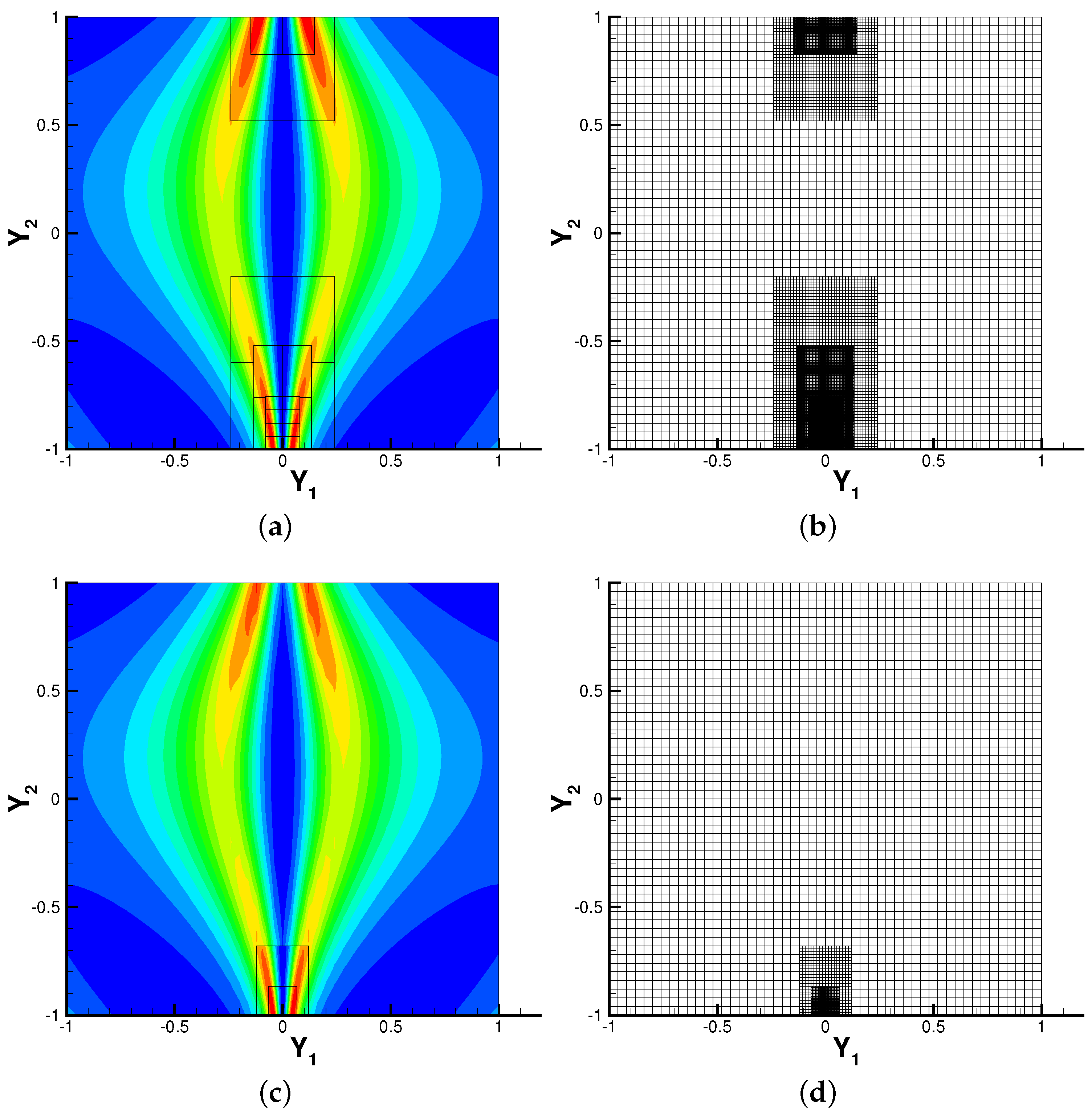
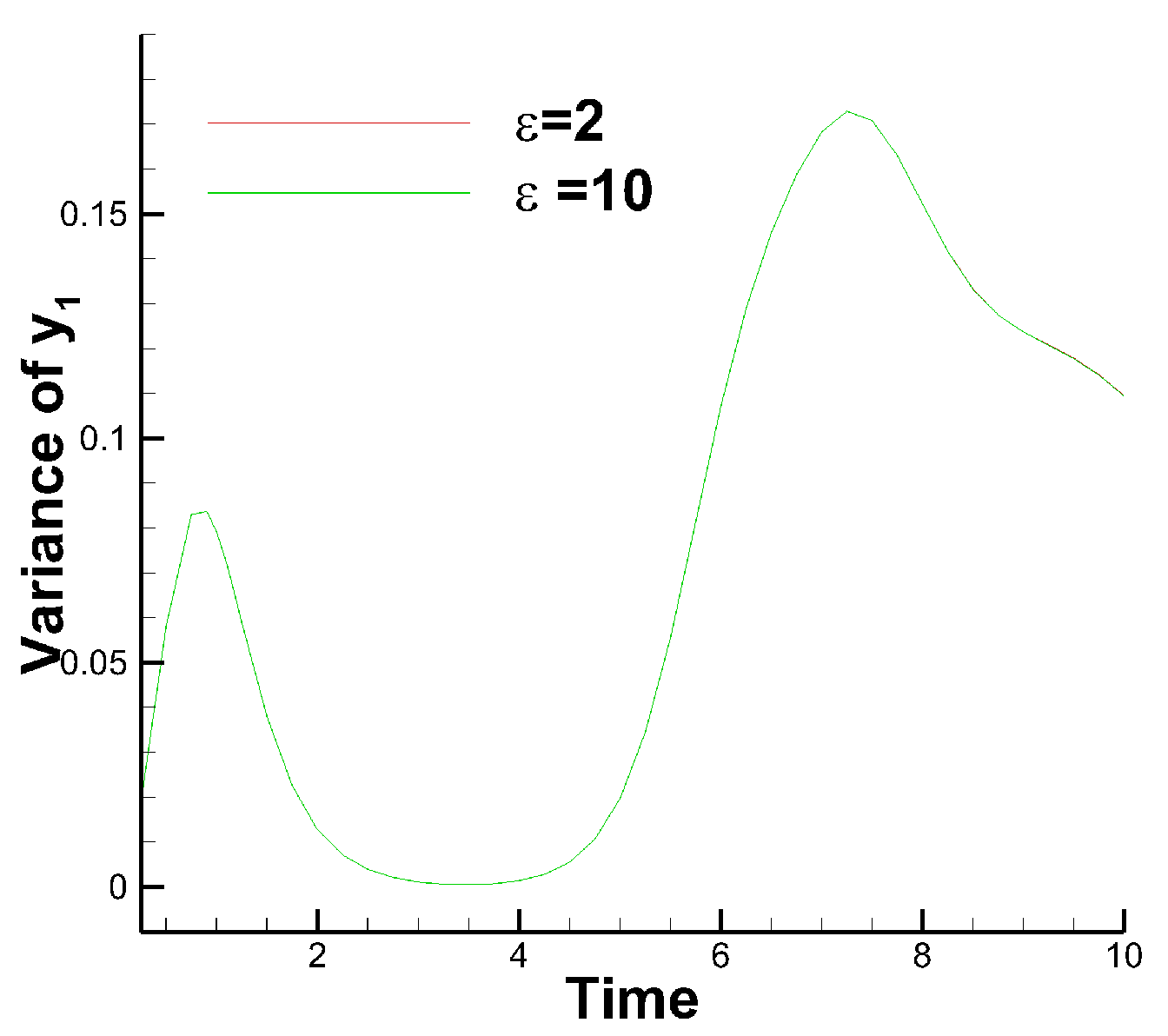
3.2. Two-Dimensional Kraichnan-Orszag (K-O) Problem

In this subsection, we consider the following transformed two-dimensional K–O three-mode problem:

$$\begin{array}{cc}\hfill \frac{d{y}_1}{dt}& =y_1{y}_3\hfill \\ \hfill \frac{d{y}_2}{dt}& =-y_2{y}_3\hfill \\ \hfill \frac{d{y}_3}{dt}& =-y_1^2+y_2^2\hfill \end{array}$$

subject to the random initial condition

$$y_1\left(0\right)=1,y_2\left(0\right)=0.1Y_1(0;\omega ),y_3\left(0\right)=Y_2(0;\omega )$$

Similar to [26], we let $Y_1$ and $Y_2$ have the uniform distribution $Y_1,Y_2\sim U(-1,1)$. The stochastic simulation for this benchmark problem is challenging since the solution exhibits a bifurcation on the parameter $y_1\left(0\right)$ and $y_2\left(0\right)$ [16]. Note that a direct application of gPC will result in failure in convergence after a short period of time. Here, we would like to use this example to further demonstrate the performance of the AMR WENO stochastic collocation scheme. The maximum mesh level is set to four and a classic forth order Runge–Kutta method with time step 0.01 is used to solve the differential equations. First, we plot the numerical solution of $y_1$ in the random space at $T=10$ with $ϵ=2,10$ and the associated adaptive mesh in Figure 6. The number of points sampled in the simulation is 29,460 and 3684 for $ϵ=2,10$, respectively. It is observed that the local mesh refinement is carried out around the line $Y_1=0$, where discontinuity occurs (see [16] for more details about the singularity of the K-O problem). We further report the time evolution of the variance of $y_1$ with $ϵ=2,10$ in Figure 7. Little difference is observed for the two simulations. For brevity, we do not report the results for $y_2$ and $y_3$, yet similar observations can be obtained. We remark that the numerical results reported agree well with the benchmarks in the literature [26].

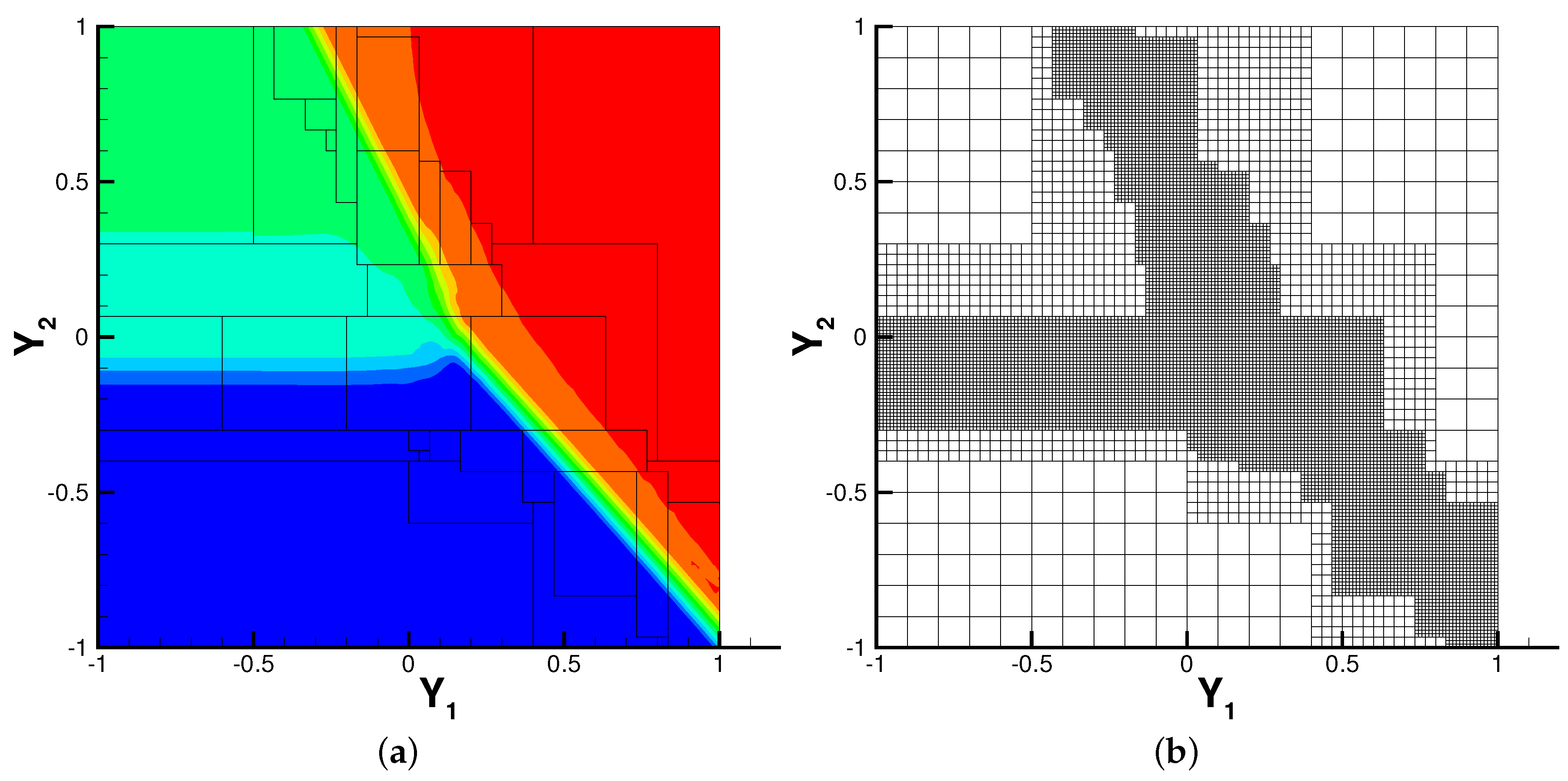
3.3. Burgers’ Equation with Random Initial Conditions

The last example we consider in this paper is the inviscid one-dimensional Burgers’ equation:

$$u_t+{\left(\frac{u^2}{2}\right)}_x=0,x\in [0,1]$$

with the following random initial condition

$$\left\{\begin{array}{cc}u(0,x)=12+0.2Y_1\hfill & x\in [0,0.3]\hfill \\ u(0,x)=6+0.2Y_2\hfill & x\in (0.3,0.6]\hfill \\ u(0,x)=3\hfill & x\in (0.6,1]\hfill \end{array}\right.$$

where $Y_1$ and $Y_2$ have the uniform distribution $Y_1,Y_2\sim U[-1,1]$. Note that there are three states for the initial condition. As time evolves, the solution will develop two shocks with different speed. After some time, the two shocks will interact with each other and finally form one single shock. It is quite challenging to simulate this problem, since this numerical solution is discontinuous in both physical and random space. Below, we will apply the proposed AMR WENO stochastic collocation method to solve this problem. We use a fifth order finite difference WENO scheme coupled with a third order SSP Runge–Kutta method to solve Burgers’ equation, which is known as a highly accurate and robust numerical scheme for solving general hyperbolic conservation laws [28]. The numerical solution is computed up to $T=0.0543$. In Figure 8, we report the contour plots of solution u in the random space with $ϵ=1,5$ at location $x=0.79$, where the shock interaction occurs. The associated adaptive meshes are also provided. Again, it is observed that the local mesh refinement is carried out around the discontinuities of the solution in the random space.

4. Conclusions and Discussion

In this paper, we developed an adaptive high-order AMR WENO-based multi-element stochastic collocation method for differential equations with random coefficients and non-smooth solutions, which consists of two important components including a WENO interpolation methodology and an AMR stochastic domain decomposition framework in random space. The numerical experiments were performed for several benchmark tests and the efficacy and efficiency of the proposed method was verified. The scheme is based on a tensor-product construction and hence suffers from the “curse of dimensionality”. Future work is to couple the AMR and WENO methodologies in random space with sparse grid [23,26] and adaptive Analysis Of Variance (ANOVA) [11,18] techniques which are efficient tools known for approximating high-dimensional problems.

References

1. Lin, G.; Su, C.-H.; Karniadakis, G.E. Random roughness enhances lift in supersonic flow. Phys. Rev. Lett. 2007, 99, 104501. [Google Scholar] [CrossRef] [PubMed]
2. Lin, G.; Su, C.-H.; Karniadakis, G.E. Stochastic modeling of random roughness in shock scattering problems: Theory and simulations. Comput. Methods Appl. Mech. Eng. 2008, 197, 3420–3434. [Google Scholar] [CrossRef]
3. Xiu, D.; Karniadakis, G.E. The Wiener-Askey polynomial chaos for stochastic differential equations. SIAM J. Sci. Comput. 2002, 24, 619–644. [Google Scholar] [CrossRef]
4. Ghanem, R.G.; Spanos, P.D. Stochastic Finite Elements: A Spectral Approach; Springer-Verlag: New York, NY, USA, 1991. [Google Scholar]
5. Babuška, I.; Nobile, F.; Tempone, R. A stochastic collocation method for elliptic partial differential equations with random input data. SIAM Rev. 2010, 52, 317–355. [Google Scholar] [CrossRef]
6. Ganapathysubramanian, B.; Zabaras, N. Sparse grid collocation schemes for stochastic natural convection problems. J. Comput. Phys. 2007, 225, 652–685. [Google Scholar] [CrossRef]
7. Hampton, J.; Doostan, A. Compressive sampling of polynomial chaos expansions: Convergence analysis and sampling strategies. J. Comput. Phys. 2015, 280, 363–386. [Google Scholar] [CrossRef]
8. Jakeman, J.D.; Eldred, M.S.; Sargsyan, K. Enhancing 1-minimization estimates of polynomial chaos expansions using basis selection. J. Comput. Phys. 2015, 289, 18–34. [Google Scholar] [CrossRef]
9. Karagiannis, G.; Konomi, B.A.; Lin, G. A bayesian mixed shrinkage prior procedure for spatial-stochastic basis selection and evaluation of gpc expansions: Applications to elliptic SPDEs. J. Comput. Phys. 2015, 284, 528–546. [Google Scholar] [CrossRef]
10. Lei, H.; Yang, X.; Zheng, B.; Lin, G.; Baker, N. Constructing surrogate models of complex systems with enhanced sparsity: Quantifying the influence of conformational uncertainty in biomolecular solvation. Multiscale Model. Simul. 2015, 13, 1327–1353. [Google Scholar] [CrossRef] [PubMed]
11. Ma, X.; Zabaras, N. An adaptive high-dimensional stochastic model representation technique for the solution of stochastic partial differential equations. J. Comput. Phys. 2010, 229, 3884–3915. [Google Scholar] [CrossRef]
12. Peng, J.; Hampton, J.; Doostan, A. A weighted ℓ1-minimization approach for sparse polynomial chaos expansions. J. Comput. Phys. 2014, 267, 92–111. [Google Scholar] [CrossRef]
13. Sargsyan, K.; Safta, C.; Najm, H.N.; Debusschere, B.J.; Ricciuto, D.; Thornton, P. Dimensionality reduction for complex models via bayesian compressive sensing. Int. J. Uncertain. Quantif. 2014, 4, 63–93. [Google Scholar] [CrossRef]
14. Tang, G.; Iaccarino, G. Subsampled gauss quadrature nodes for estimating polynomial chaos expansions. SIAM J. Uncertain. Quantif. 2014, 2, 423–443. [Google Scholar] [CrossRef]
15. Xu, Z.; Zhou, T. On sparse interpolation and the design of deterministic interpolation points. SIAM J. Sci. Comput. 2014, 36, A1752–A1769. [Google Scholar] [CrossRef]
16. Wan, X.; Karniadakis, G.E. An adaptive multi-element generalized polynomial chaos method for stochastic differential equations. J. Comput. Phys. 2005, 209, 617–642. [Google Scholar] [CrossRef]
17. Wan, X.; Karniadakis, G.E. Multi-element generalized polynomial chaos for arbitrary probability measures. SIAM J. Sci. Comput. 2006, 28, 901–928. [Google Scholar] [CrossRef]
18. Foo, J.; Karniadakis, G.E. Multi-element probabilistic collocation method in high dimensions. J. Comput. Phys. 2010, 229, 1536–1557. [Google Scholar] [CrossRef]
19. Foo, J.; Wan, X.; Karniadakis, G.E. The multi-element probabilistic collocation method (ME-PCM): Error analysis and applications. J. Comput. Phys. 2008, 227, 9572–9595. [Google Scholar] [CrossRef]
20. Archibald, R.; Gelb, A.; Saxena, R.; Xiu, D. Discontinuity detection in multivariate space for stochastic simulations. J. Comput. Phys. 2009, 228, 2676–2689. [Google Scholar] [CrossRef]
21. Bilionis, I.; Zabaras, N.; Konomi, B.; Lin, G. Multi-output separable gaussian process: Towards an efficient, fully bayesian paradigm for uncertainty quantification. J. Comput. Phys. 2013, 241, 212–239. [Google Scholar] [CrossRef]
22. Chantrasmi, T.; Doostan, A.; Iaccarino, G. Pade-legendre approximants for uncertainty analysis with discontinuous response surface. J. Comput. Phys. 2009, 228, 7159–7180. [Google Scholar] [CrossRef]
23. Jakeman, J.; Archibald, R.; Xiu, D. Characterization of discontinuities in high-dimensional stochastic problmes on adaptive sparse grids. J. Comput. Phys. 2011, 230, 3977–3997. [Google Scholar] [CrossRef]
24. Jakeman, J.; Narayan, A.; Xiu, D. Minimal multi-element stochastic collocation for uncertainty quantification of discontinuous functions. J. Comput. Phys. 2013, 242, 790–808. [Google Scholar] [CrossRef]
25. Konomi, B.; Karagiannis, G.; Sarkar, A.; Lin, G. Bayesian treed multivariate gaussian process with adaptive design: Application to a carbon capture unit. Technometrics 2014, 56, 145–158. [Google Scholar] [CrossRef]
26. Ma, X.; Zabaras, N. An adaptive hierarchical sparse grid collocation algorithm for the solution of stochastic differential equations. J. Comput. Phys. 2009, 228, 3084–3113. [Google Scholar] [CrossRef]
27. Shen, C.; Qiu, J.-M.; Christlieb, A. Adaptive mesh refinement based on high order finite difference WENO scheme for multi-scale simulations. J. Comput. Phys. 2011, 230, 3780–3802. [Google Scholar] [CrossRef]
28. Shu, C.-W. High order weighted essentially nonoscillatory schemes for convection dominated problems. SIAM Rev. 2009, 51, 82–126. [Google Scholar] [CrossRef]
29. Qiu, J.; Shu, C.-W. Runge-Kutta discontinuous Galerkin method using WENO limiters. SIAM J. Sci. Comput. 2005, 26, 907–929. [Google Scholar] [CrossRef]
30. Tan, S.; Shu, C.-W. Inverse Lax-Wendroff procedure for numerical boundary conditions of conservation laws. J. Comput. Phys. 2010, 229, 8144–8166. [Google Scholar] [CrossRef]
31. Berger, M.; Colella, P. Local adaptive mesh refinement for shock hydrodynamics. J. Comput. Phys. 1989, 82, 64–84. [Google Scholar] [CrossRef]
32. Berger, M.; Oliger, J. Adaptive mesh refinement for hyperbolic partial differential equations. J. Comput. Phys. 1984, 53, 484–512. [Google Scholar] [CrossRef]
33. Berger, M.; Rigoutsos, I. An algorithm for point clustering and grid generation. IEEE Trans. Syst. Man Cybern. 1991, 21, 1278–1286. [Google Scholar] [CrossRef]
Figure 1. One-dimensional WENO interpolation.
Mathematics 04 00029 g001
Figure 2. Two-dimensional WENO interpolation.
Mathematics 04 00029 g002
Figure 3. Two-dimensional AMR WENO interpolation.
Mathematics 04 00029 g003
Figure 4. Interpolation comparison of f 1 using the WENO reconstruction. (a) interpolant function of f 1 with ϵ = 10 ; (b) AMR mesh with ϵ = 10 ; (c) interpolant function of f 1 with ϵ = 1 ; (d) AMR mesh with ϵ = 1 .
Mathematics 04 00029 g004
Figure 5. Interpolation of the discontinuous function f 2 using the WENO reconstruction. (a) Interpolant function of f 2 with ϵ = 1 ; (b) AMR mesh with ϵ = 1 .
Mathematics 04 00029 g005
Figure 6. Contour plots of solution of the K-O problem in the random space. (a) y 1 with ϵ = 2 ; (b) AMR mesh with ϵ = 2 ; (c) y 1 with ϵ = 2 ; (d) AMR mesh with ϵ = 10 .
Mathematics 04 00029 g006
Figure 7. The time evolution of the variance of y 1 .
Mathematics 04 00029 g007
Figure 8. Contour plots of solution of the one-dimensional Burgers equation in random space. (a) numerical solution with ϵ = 1 ; (b) AMR mesh with ϵ = 1 ; (c) numerical solution with ϵ = 5 ; (d) AMR mesh with ϵ = 5 .
Mathematics 04 00029 g008aMathematics 04 00029 g008b