Dynamic Cooperative Oligopolies

Abstract

An n-person cooperative oligopoly is considered without product differentiation. It is assumed that the firms know the unit price function but have no access to the cost functions of the competitors. From market data, they have information about the industry output. The firms want to find the output levels that guarantee maximum industry profit. First, the existence of a unique maximizer is proven, which the firms cannot determine directly because of the lack of the knowledge of the cost functions. Instead, a dynamic model is constructed, which is asymptotically stable under realistic conditions, and the state trajectories converge to the optimum output levels of the firms. Three models are constructed: first, no time delay is assumed; second, information delay is considered for the firms on the industry output; and third, in addition, information delay is also assumed about the firms’ own output levels. The stability of the resulting no-delay, one-delay, and two-delay dynamics is examined.

1. Introduction

Based on the pioneering work of Cournot A. [1], an intensive study on his oligopoly model started, which continues until today. Most studies consider this model as a multiplayer non-cooperative game. First, the existence and uniqueness of the Nash equilibrium were the main research subjects [2,3]. Several versions of oligopolies were introduced and studied, including models with product differentiation, multi-product, labor-managed oligopolies, oligopsonies, and group equilibrium problems, among others [4]. In dynamic extensions, first linear models were studied since local and global asymptotic stability are equivalent [5,6]. Based on the mathematical development of nonlinear dynamics, oligopolies with nonlinear payoff functions have become the main focus [7,8,9]. In recent years, oligopolies with time delays have been receiving increasing attention, since data collection in order to determine the best decisions and their implementations need time. If the delay is due to contractual or institutional circumstances, then fixed delays are considered. If the delays are uncertain due to the large number of firms, or the firms want to react to an average of past information rather than to sudden market changes, then continuously distributed delays are assumed. In the first case, differential–difference equations model the situation [10], whereas in the second case, integro-differential equations model the situation [11]. In the past, oligopoly studies of mainly non-cooperative models were considered, and the Nash equilibrium in static games or the steady states of the dynamic models were the focus. In the case of cooperative games, the players want to obtain maximum overall profit, which is then distributed among them based on certain fairness principles [12]. Several concepts and methods were developed [13], among which the Shapley values are the most popular [14].

Many applications of non-cooperative games are known from the literature, which can be found in many text books, like [15]. The applications of cooperative games also cover a huge and diverse field in applied sciences, including natural resource management [16,17], power systems [18], waste management [19], transportation [20,21], insurance industry [22], social network analysis [23], communication network [24], manufacturing systems [25], pattern clustering [26], and business and economics [27], among others. In this paper, n-person oligopolies without product differentiation will be considered and examined under the assumption that the firms know the unit price function and are able to obtain information about the industry output; however, they do not know the cost functions of the others since no technology information is shared among the players. Therefore, they cannot determine their total industry profit maximizing output levels. Hence, an asymptotically stable dynamic process is assumed in which the steady state gives the optimal output levels.

The paper is developed as follows. In Section 2, the basic model is outlined, and in Section 3, its dynamic extension is examined without time delays. Two-delay models are introduced and analyzed in Section 4. In the first case, data on the industry output are assumed to be delayed, and in the second case, in addition, data on the firms’ own output levels are also considered delayed. The model without delay is asymptotically stable under realistic conditions. In the single delay case, it is asymptotically stable if the length of the delay is smaller than a threshold value, where stability is lost by Hopf bifurcation. In the two-delay case, the stability switching curve is determined in the delays’ space. Section 5 offers concluding remarks and outlines further research directions.

2. The Basic Model

In a cooperative oligopoly, the firms want to maximize their overall profit:

$$\phi (x_1,x_2,\dots ,x_n)=sp\left(s\right)-\sum _{k=1}^n{C}_k\left(x_k\right).$$

(1)

Here, $x_k$ is the output of firm k with $0\le x_k\le L_k$, where $L_k$ is the capacity limit of this firm. Furthermore, $s={\sum }_{k=1}^n{x}_k,p\left(s\right)$ is the price function and $C_k\left(x_k\right)$ is the cost function of firm k. Assume that functions p and all $C_k$ values are twice continuously differentiable; then

$$\begin{array}{c}\left(A\right)p^{\prime }\left(s\right)<0\mathrm{for}0\le s\le \sum _{k=1}^n{L}_k,\hfill \\ \left(B\right)p^{\prime }\left(s\right)+s{p}^{″}\left(s\right)\le 0\mathrm{for}0\le s\le \sum _{k=1}^n{L}_k,\hfill \\ \left(C\right)C_k^{\prime }\left(x_k\right)>0,C_k^{″}\left(x_k\right)>0\mathrm{for}0\le x_k\le L_k \mathrm{and} \mathrm{all} k.\hfill \end{array}$$

Notice that

$${\displaystyle \frac{\partial \phi }{\partial x_k}}=s{p}^{\prime }\left(s\right)+p\left(s\right)-C_k^{\prime }\left(x_k\right),$$

(2)

$${\displaystyle \frac{{\partial }^2\phi }{\partial x_k^2}}=s{p}^{″}\left(s\right)+2p^{\prime }\left(s\right)-C_k^{″}\left(x_k\right)$$

and for $k\ne \ell ,$

$${\displaystyle \frac{{\partial }^2\phi }{\partial x_k\partial x_{\ell }}}=s{p}^{″}\left(s\right)+2p^{\prime }\left(s\right).$$

Introduce matrices

$$\mathit{A}=\left(\begin{array}{cccc}1& 1& ···& 1\\ 1& 1& ···& 1\\ ·& ·& ···& ·\\ 1& 1& ···& 1\end{array}\right)\mathrm{and}\mathit{B}=\left(\begin{array}{cccc}-C_1^{″}\left(x_1\right)& 0& ···& 0\\ 0& -C_2^{″}\left(x_2\right)& ···& 0\\ ·& ·& ···& ·\\ 0& 0& ···& -C_n^{″}\left(x_n\right)\end{array}\right),$$

then, the Hessian matrix of $\phi$ can be written as

$$\mathit{H}=\left(s{p}^{″}\left(s\right)+2p^{\prime }\left(s\right)\right)\mathit{A}+\mathit{B}.$$

(3)

Here, $\mathit{B}$ is a negative definite, and eigenvalues of $\mathit{A}$ are 0 and n; furthermore,

$$s{p}^{″}\left(s\right)+2p^{\prime }\left(s\right)=p^{\prime }\left(s\right)+s{p}^{″}\left(s\right)+p^{\prime }\left(s\right)<0.$$

Therefore, $\mathit{H}$ is negative definite, implying that $\phi$ is strictly concave as an n-variable function.

Since $s{p}^{″}\left(s\right)+2p^{\prime }\left(s\right)$ is the derivative of $s{p}^{\prime }\left(s\right)+p\left(s\right),$ this function is strictly decreasing in s. With given $s\ge 0,$ the best choice of firm k is given as continuous function:

$$R_k\left(s\right)=\left\{\begin{array}{c}0\mathrm{if}s{p}^{\prime }\left(s\right)+p\left(s\right)-C_k^{\prime }\left(0\right)\le 0,\hfill \\ L_k\mathrm{if}s{p}^{\prime }\left(s\right)+p\left(s\right)-C_k^{\prime }\left(L_k\right)\ge 0,\hfill \\ x_k^{*}\mathrm{otherwise},\hfill \end{array}\right.$$

(4)

where $x_k^{*}$ solves the equation

$$h\left(x_k\right)=s{p}^{\prime }\left(s\right)+p\left(s\right)-C_k^{\prime }\left(x_k\right)=0.$$

(5)

In the third case of (4), $h\left(x_k\right)$ strictly decreases in $x_k,$ $h\left(0\right)>0$ and $h\left(L_k\right)<0$. Therefore, there is a unique solution of Equation (5). It is easy to show that $R_k\left(s\right)$ is a non-increasing continuous function of s.

Consider finally the following equation:

$$g\left(s\right)=\sum _{k=1}^n{R}_k\left(s\right)-s=0.$$

(6)

The left hand-side strictly decreases:

$$g\left(0\right)\ge 0\mathrm{and}g\left(\sum _{k=1}^n{L}_k\right)\le 0.$$

Therefore, there is a unique solution $s^{*}>0$ of (6) and then the optimal choices of the firms are given by (4) as

$$x_k^{*}=R_k\left(s^{*}\right).$$

3. Dynamic Extension

Using gradient adjustments, the output adjustments are generally driven by the differential equations:

$$\begin{array}{cc}{\dot{x}}_k\left(t\right)\hfill & =K_k\left[s\left(t\right)p^{\prime }\left(s\left(t\right)\right)+p\left(s\left(t\right)\right)-C_k^{\prime }\left(x_k\left(t\right)\right)\right]\hfill \\ \hfill & =K_k\left[\left(\sum _{\ell =1}^n{x}_{\ell }\left(t\right)\right)p^{\prime }\left(\sum _{\ell =1}^n{x}_{\ell }\left(t\right)\right)+p\left(\sum _{\ell =1}^n{x}_{\ell }\left(t\right)\right)-C_k^{\prime }\left(x_k\left(t\right)\right)\right].\hfill \end{array}$$

(7)

The right hand-side is a constant multiple of the marginal profit with $K_k>0$. Notice that

$$\begin{array}{cc}{\displaystyle \frac{\partial {\dot{x}}_k\left(t\right)}{\partial x_k}}\hfill & =K_k\left\{2p^{\prime }\left(\sum _{\ell =1}^n{x}_{\ell }\left(t\right)\right)+\left(\sum _{\ell =1}^n{x}_{\ell }\left(t\right)\right)p^{″}\left(\sum _{\ell =1}^n{x}_{\ell }\left(t\right)\right)-C_k^{″}\left(x_k\left(t\right)\right)\right\}\hfill \\ \hfill & =K_k\left[2p^{\prime }\left(s\left(t\right)\right)+s\left(t\right)p^{″}\left(s\left(t\right)\right)-C_k^{″}\left(x_k\left(t\right)\right)\right]\hfill \end{array}$$

(8)

and for $\ell \ne k$,

$${\displaystyle \frac{\partial {\dot{x}}_k\left(t\right)}{\partial x_{\ell }}}=K_k\left(2p^{\prime }\left(s\left(t\right)\right)+s\left(t\right)p^{″}\left(s\left(t\right)\right)\right).$$

(9)

The Jacobian of this system is clearly

$$\mathit{J}=\mathit{KH}$$

with

$$\mathit{K}=diag\left(K_1,K_2,\dots ,K_n\right).$$

It is well known that all eigenvalues of $\mathit{J}$ have negative real parts (see Theorem 4.9 of Szidarovszky and Bahill [28], implying the local asymptotical stability of the optimal solution without delays).

Theorem 1.

The steady state of system (7) is always locally asymptotically stable.

4. Dynamic Extension with Time Delay

Assume next that the firms have delayed information about the industry output. If ${\tau }_k$ is the delay for firm k, then Equation (7) is modified as follows:

$${\dot{x}}_k\left(t\right)=K_k\left[s_k{p}^{\prime }\left(s_k\right)+p\left(s_k\right)-C_k^{\prime }\left(x_k\left(t\right)\right)\right]$$

(10)

with

$$s_k=\sum _{\ell =1}^n{x}_{\ell }(t-{\tau }_k)$$

Notice that

$${\displaystyle \frac{\partial {\dot{x}}_k\left(t\right)}{\partial s_k}}=K_k\left[s_k{p}^{″}\left(s_k\right)+2p^{\prime }\left(s_k\right)\right]$$

and

$${\displaystyle \frac{\partial {\dot{x}}_k\left(t\right)}{\partial x_k}}=-K_k{C}_k^{″}\left(x_k\left(t\right)\right).$$

Let $s^{*}$ and $x_k^{*}$ denote the values of s and $x_k$ at the optimal solution. Clearly

$$s^{*}=\sum _{k=1}^n{x}_k^{*}.$$

Introduce the notation

$$A=s^{*}{p}^{″}\left(s^{*}\right)+2p^{\prime }\left(s^{*}\right)$$

and

$$B_k=-C_k^{″}\left(x_k^{*}\right),$$

then, the linearized homogenous equation is as follows:

$${\dot{x}}_k\left(t\right)=K_{k}A\sum _{\ell =1}^n{x}_{\ell }(t-{\tau }_k)+K_k{B}_k{x}_k\left(t\right).$$

(11)

Upon examining the stability of the equilibrium of this system, we will use the methodology offered by Bellman and Cooke [10].

Notice that A and all $B_k$ values are negative. Assume exponential solutions results in $x_k\left(t\right)=e^{\lambda t}{u}_k$ to have

$$\lambda u_k=K_{k}A\sum _{\ell =1}^n{e}^{-\lambda {\tau }_k}{u}_{\ell }+K_k{B}_k{u}_k\mathrm{for}k=1,2,\dots ,n$$

showing that the characteristic equation becomes

$$det\left(\begin{array}{cccc}\lambda -K_{1}A{e}^{-\lambda {\tau }_1}-K_1{B}_1& -K_{1}A{e}^{-\lambda {\tau }_1}& ···& -K_{1}A{e}^{-\lambda {\tau }_1}\\ -K_{2}A{e}^{-\lambda {\tau }_2}& \lambda -K_{2}A{e}^{-\lambda {\tau }_2}-K_2{B}_2& ···& -K_{2}A{e}^{-\lambda {\tau }_2}\\ ·& ·& ···& ·\\ -K_{n}A{e}^{-\lambda {\tau }_n}& -K_{n}A{e}^{-\lambda {\tau }_n}& ···& \lambda -K_{n}A{e}^{-\lambda {\tau }_n}-K_n{B}_n\end{array}\right)=0.$$

(12)

It can be represented in closed form based on the result given in Appendix E of Bischi et al.’s work [29]. Introduce

$$\mathit{a}=\left(\begin{array}{c}-K_{1}A{e}^{-\lambda {\tau }_1}\\ -K_{2}A{e}^{-\lambda {\tau }_2}\\ ·\\ -K_{n}A{e}^{-\lambda {\tau }_n}\end{array}\right),{\mathbf{1}}^T=\left(1,1,\dots ,1\right)$$

and

$$\mathit{D}=diag\left(\lambda -K_1{B}_1,\lambda -K_2{B}_2,\dots ,\lambda -K_n{B}_n\right)$$

to have (12) in the following form:

$$\begin{array}{cc}det\left(\mathit{D}+\mathit{a}{\mathbf{1}}^T\right)\hfill & =det\left(\mathit{D}\right)det\left(\mathit{I}+{\mathit{D}}^{-1}\mathit{a}{\mathbf{1}}^T\right)\hfill \\ \hfill & =det\left(\mathit{D}\right)det\left[1+{\mathbf{1}}^T{\mathit{D}}^{-1}\mathit{a}\right]\hfill \\ \hfill & ={\mathrm{\Pi }}_{k=1}^n\left(\lambda -K_k{B}_k\right)\left[1-\sum _{k=1}^n{\displaystyle \frac{K_{k}A{e}^{-\lambda {\tau }_k}}{\lambda -K_k{B}_k}}\right]=0.\hfill \end{array}$$

From the first factor,

$$\lambda =K_k{B}_k<0,$$

which does not disturb stability. The expression inside the brackets is very difficult to deal with in general, so we make the following simplifying assumption:

$$\left(D\right)K_1=K_2=\dots =K_n=K,B_1=B_2=\dots =B_n=B\mathrm{and}{\tau }_1={\tau }_2=\dots ={\tau }_n=\tau .$$

In this special case, we have to examine the following equation

$$1-\sum _{k=1}^n{\displaystyle \frac{KA{e}^{-\lambda \tau }}{\lambda -KB}}=0$$

or

$$\lambda -KB-nKA{e}^{-\lambda \tau }=0.$$

(13)

Without delay, $\tau =0$ and $\lambda =KB+nKA<0$. Stability switch might occur if $\lambda =i\omega \left(\omega >0\right)$, which is now substituted into Equation (13) to have

$$i\omega -KB-nKA\left(\cos \omega \tau -i\sin \omega \tau \right)=0.$$

Separating the real and imaginary parts gives

$$nKA\cos \omega \tau =-KB$$

(14)

and

$$nKA\sin \omega \tau =-\omega .$$

(15)

Adding the squares of these equations, we have

$${\omega }^2=K^2\left(n^2{A}^2-B^2\right).$$

Theorem 2.

If $n^2{A}^2\le B^2$, then no stability switch occurs, and optimal solution is locally asymptotically stable for all $\tau \ge 0$.

Assume next that $n^2{A}^2>B^2$, then

$${\omega }^{*}=K\sqrt{n^2{A}^2-B^2}.$$

From (14) and (15), we see that $cos\omega \tau <0$ and $sin\omega \tau >0$, implying that

$${\tau }_m=\frac{1}{{\omega }^{*}}\left(\pi -{sin}^{-1}\left(\frac{-{\omega }^{*}}{nKA}\right)+2m\pi \right)m=0,1,2,\dots$$

(16)

The directions of the stability switches are obtained by Hopf bifurcation. Select $\tau$ as the bifurcation parameter and assume $\lambda =\lambda \left(\tau \right)$. Implicitly differentiating Equation (13) with respect to $\tau ,$ we have

$${\lambda }^{\prime }-nKA{e}^{-\lambda \tau }\left(-{\lambda }^{\prime }\tau -\lambda \right)=0$$

so

$${\lambda }^{\prime }=\frac{-nKA{e}^{-\lambda \tau }\lambda }{1+nKA{e}^{-\lambda \tau }\tau }=\frac{-\left(\lambda -KB\right)\lambda }{1+\left(\lambda -KB\right)\tau }.$$

With $\lambda =i\omega$, the real part is

$$\begin{array}{ccc}\hfill \mathrm{Re}\left[{\left.{\lambda }^{\prime }\right|}_{\lambda =i\omega }\right]& =& \mathrm{Re}\left[\frac{{\omega }^2+iKB\omega }{1-KB\tau +i\omega \tau }\right]\hfill \\ & =& \frac{{\omega }^2}{{\left(1-KB\tau \right)}^2+{\left(\omega \tau \right)}^2}>0.\hfill \end{array}$$

Theorem 3.

If $n^2{A}^2>B^2,$ then the optimal solution is locally asymptotically stable for $\tau <{\tau }_0,$ stability is lost at $\tau ={\tau }_0$ with Hopf bifurcation, and stability cannot be regained with larger values of τ.

In addition to Assumption (D), assume that the firms have an identical delay ${\tau }_1$ in the industry output and an identical delay ${\tau }_2$ in their own output values. Then, Model (10) is modified as follows:

$${\dot{x}}_k\left(t\right)=K\left[s{p}^{\prime }\left(s\right)+p\left(s\right)-C_k^{\prime }\left(x_k(t-{\tau }_2)\right)\right]$$

(17)

with

$$s=\sum _{\ell =1}^n{x}_{\ell }(t-{\tau }_1).$$

This is a system of two-delay equations. The stability of its equilibrium will be examined by the method offered by Matsumoto and Szidarovszky [30] based on Gu et al. [31].

The linearized equation is now the following:

$${\dot{x}}_k\left(t\right)=KA\sum _{\ell =1}^n{x}_{\ell }(t-{\tau }_1)+KB{x}_k(t-{\tau }_2).$$

(18)

Assuming exponential solutions $x_{\ell }\left(t\right)=e^{\lambda t}{u}_{\ell }$, we then obtain by substitution

$$\left(\lambda -KB{e}^{-\lambda {\tau }_2}\right)u_k-KA\sum _{\ell =1}^n{e}^{-\lambda {\tau }_1}{u}_{\ell }=0,$$

implying that the characteristic equation has the form

$$det\left(\begin{array}{cccc}\lambda -KA{e}^{-\lambda {\tau }_1}-KB{e}^{-\lambda {\tau }_2}& -KA{e}^{-\lambda {\tau }_1}& ···& -KA{e}^{-\lambda {\tau }_1}\\ -KA{e}^{-\lambda {\tau }_1}& \lambda -KA{e}^{-\lambda {\tau }_1}-KB{e}^{-\lambda {\tau }_2}& ···& -KA{e}^{-\lambda {\tau }_1}\\ ·& ·& ···& ·\\ -KA{e}^{-\lambda {\tau }_1}& -KA{e}^{-\lambda {\tau }_1}& ·& \lambda -KA{e}^{-\lambda {\tau }_1}-KB{e}^{-\lambda {\tau }_2}\end{array}\right)=0.$$

(19)

Let $\mathbf{1}$ be again the n-element vector with all unity elements, and $\mathit{I}$ be the $n\times n$ identity matrix. Then, (19) can be rewritten as

$$\begin{array}{cc}det\left(\mathit{D}+\mathit{a}{\mathbf{1}}^T\right)\hfill & =det\left(\mathit{D}\right)det\left(\mathit{I}+{\mathit{D}}^{-1}\mathit{a}{\mathbf{1}}^T\right)\hfill \\ \hfill & =det\left(\mathit{D}\right)det\left[1+{\mathbf{1}}^T{\mathit{D}}^{-1}\mathit{a}\right]\hfill \\ \hfill & ={\left(\lambda -KB{e}^{-\lambda {\tau }_2}\right)}^n\left[1-\sum _{k=1}^n{\displaystyle \frac{KA{e}^{-\lambda {\tau }_1}}{\lambda -KB{e}^{-\lambda {\tau }_2}}}\right]=0,\hfill \end{array}$$

(20)

where

$$\mathit{a}=-KA{e}^{-\lambda {\tau }_1}\mathbf{1}\mathrm{and}\mathit{D}=\left(\lambda -KB{e}^{-\lambda {\tau }_2}\right)\mathit{I}.$$

Thus, we have two-delay equations:

$$\lambda -KB{e}^{-\lambda {\tau }_2}=0$$

(21)

and

$$\lambda -K\left(nA{e}^{-\lambda {\tau }_1}+B{e}^{-\lambda {\tau }_2}\right)=0.$$

(22)

Notice that (21) is a single-delay equation, and at ${\tau }_2=0$, the eigenvalue is $\lambda =KB<0$. The sign of the real part of the eigenvalue might change at $\lambda =i\omega .$ Then

$$i\omega -KB\left(\cos \omega {\tau }_2-i\sin \omega {\tau }_2\right)=0.$$

Separation of the real and imaginary parts shows that

$$KBcos\omega {\tau }_2=0$$

(23)

and

$$KBsin\omega {\tau }_2=-\omega ,$$

(24)

implying that

$$cos\omega {\tau }_2=0\mathrm{and}sin\omega {\tau }_2=1,$$

and the critical values of ${\tau }_2$ are

$${\tau }_{2n}=-\frac{1}{KB}\left(\frac{\pi }{2}+2n\pi \right)\mathrm{for}n=0,1,2,\dots$$

since, from (24), $\omega =-KB$. The directions of stability switches are determined by Hopf bifurcation, when ${\tau }_2$ is selected as the bifurcation parameter and let $\lambda =\lambda \left({\tau }_2\right)$. Implicit differentiation of Equation (21) with respect to ${\tau }_2$ shows that

$${\lambda }^{\prime }-KB{e}^{-\lambda {\tau }_2}\left(-{\lambda }^{\prime }{\tau }_2-\lambda \right)=0,$$

implying that

$${\lambda }^{\prime }=\frac{-{\lambda }^2}{1+\lambda {\tau }_2},$$

where we use $KB{e}^{-\lambda {\tau }_2}=\lambda$. At $\lambda =i\omega$, the real part of ${\lambda }^{\prime }$ is positive:

$$\begin{array}{ccc}\hfill \mathrm{Re}\left[{\lambda }^{\prime }\right]& =& \mathrm{Re}\left[\frac{{\omega }^2}{1+i\omega {\tau }_2}\right],\hfill \\ & =& \mathrm{Re}\left[\frac{{\omega }^2\left(1-i\omega {\tau }_2\right)}{1+{\left(\omega {\tau }_2\right)}^2}\right],\hfill \\ & =& \frac{{\omega }^2}{1+{\left(\omega {\tau }_2\right)}^2}>0.\hfill \end{array}$$

Therefore, the eigenvalues of Equation (21) have negative real parts for $\tau <{\tau }_{20},$ and at all critical values ${\tau }_{2n}(n=0,1,2,\dots ),$ at least one pair of eigenvalues changes the sign of its real part from negative to positive.

We now turn to Equation (22), which can be written as

$$1+a_1\left(\lambda \right)e^{-\lambda {\tau }_1}+a_2\left(\lambda \right)e^{-\lambda {\tau }_2}=0$$

with

$$a_1\left(\lambda \right)=-\frac{nKA}{\lambda }\mathrm{and}{a}_2\left(\lambda \right)=-\frac{KB}{\lambda }.$$

Notice first that without delays, $\lambda =nKA+KB<0$, and with increasing values of the delays, stability may be lost when $\lambda =i\omega .$ Then, we have

$$1+a_1\left(i\omega \right)e^{-i\omega {\tau }_1}+a_2\left(i\omega \right)e^{-i\omega {\tau }_2}=0$$

where

$$a_1\left(i\omega \right)=i\frac{nKA}{\omega },a_2\left(i\omega \right)=i\frac{KB}{\omega },$$

$$\left|a_1\left(i\omega \right)\right|=-\frac{nKA}{\omega }\mathrm{and}\left|a_2\left(i\omega \right)\right|=-\frac{KB}{\omega },$$

and

$$arg\left[a_1\left(i\omega \right)\right]=arg\left[a_2\left(i\omega \right)\right]=\frac{3\pi }{2}.$$

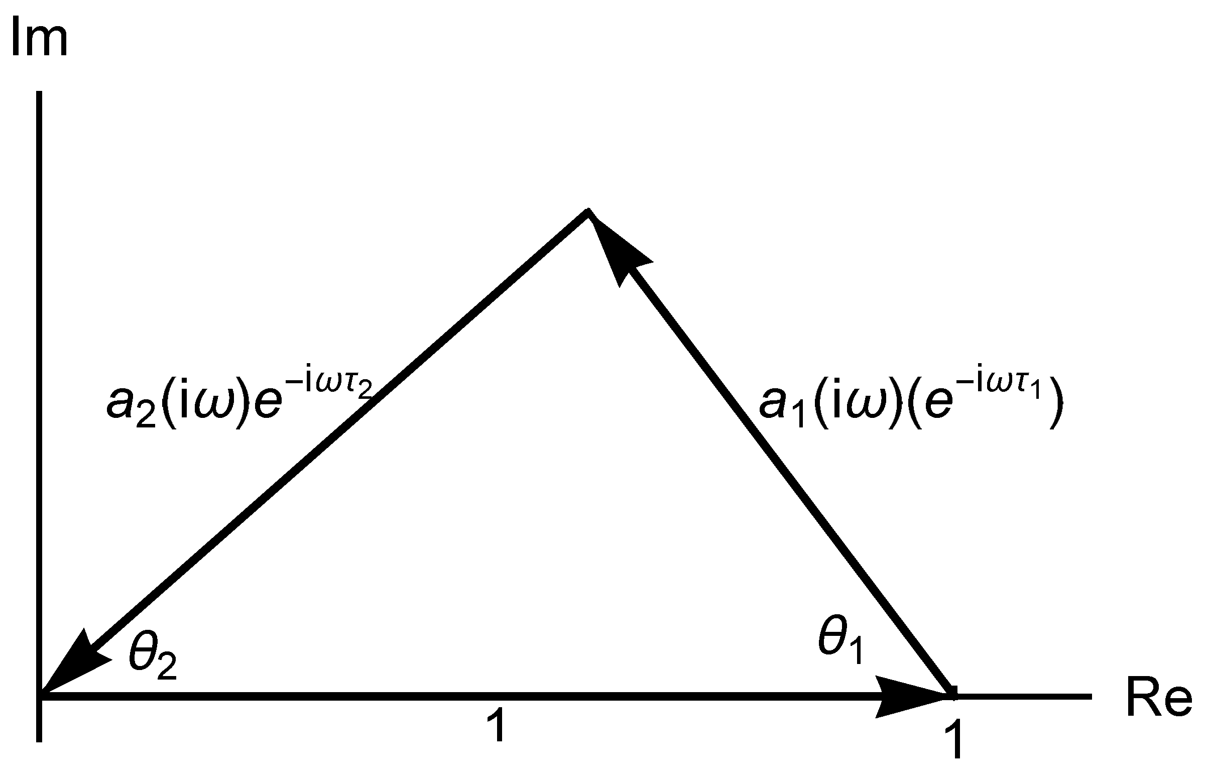
If we place vectors, $1,a_1\left(i\omega \right)e^{-i\omega {\tau }_1}$ and $a_2\left(i\omega \right)e^{-i\omega {\tau }_2}$ head to tail, then they form a triangle. The sufficient and necessary conditions for the existence of a triangle are

$$\begin{array}{c}\left|a_1\left(i\omega \right)\right|+\left|a_2\left(i\omega \right)\right|\ge 1,\\ -1\le \left|a_1\left(i\omega \right)\right|-\left|a_2\left(i\omega \right)\right|\le 1.\end{array}$$

In our case,

$$\begin{array}{c}-nKA-KB\ge \omega ,\\ -\omega \le -nKA+KB\le \omega \end{array}$$

which can be summarized as

$$\left|-nKA+KB\right|\le \omega \le -nKA-KB.$$

(25)

The triangle is illustrated in Figure 1, when the interior angles are ${\theta }_1,{\theta }_2$, and $\pi -({\theta }_1+{\theta }_2)$.

The rule of cosine shows that

$${\theta }_1={cos}^{-1}\left(\frac{1+{\left|a_1\left(i\omega \right)\right|}^2-{\left|a_2\left(i\omega \right)\right|}^2}{2\left|a_1\left(i\omega \right)\right|}\right)={cos}^{-1}\left(\frac{{\omega }^2+{\left(nKA\right)}^2-{\left(KB\right)}^2}{-2nKA\omega }\right)$$

(26)

and

$${\theta }_2={cos}^{-1}\left(\frac{1+{\left|a_2\left(i\omega \right)\right|}^2-{\left|a_1\left(i\omega \right)\right|}^2}{2\left|a_2\left(i\omega \right)\right|}\right)={cos}^{-1}\left(\frac{{\omega }^2+{\left(KB\right)}^2-{\left(nKA\right)}^2}{-2KB\omega }\right).$$

(27)

The arguments of the three sides of the triangle are

$$0,arg\left[a_1\left(i\omega \right)\right]-\omega {\tau }_1\mathrm{and}arg\left[a_2\left(i\omega \right)\right]-\omega {\tau }_2$$

and the angle balance equations at the end points of the horizontal side show that

$${\tau }_1^{k\pm }\left(\omega \right)=\frac{1}{\omega }\left[arg\left(a_1\left(i\omega \right)\right)+(2k-1)\pi \pm {\theta }_1\right]\mathrm{for}k=0,1,2,\dots$$

and

$${\tau }_2^{\ell \mp }\left(\omega \right)=\frac{1}{\omega }\left[arg\left(a_2\left(i\omega \right)\right)+(2\ell -1)\pi \mp {\theta }_2\right]\mathrm{for}\ell =0,1,2,\dots$$

since the triangle can be located above and under the horizontal axis. Hence,

$${\tau }_1^{k\pm }\left(\omega \right)=\frac{1}{\omega }\left[\frac{3\pi }{2}+(2k-1)\pi \pm {\theta }_1\right]\mathrm{for}k=0,1,2,\dots$$

(28)

and

$${\tau }_2^{\ell \mp }\left(\omega \right)=\frac{1}{\omega }\left[\frac{3\pi }{2}+(2\ell -1)\pi \mp {\theta }_2\right]\mathrm{for}\ell =0,1,2,\dots ,$$

(29)

implying that the stability switching curves are formed as

$$T_{k,\ell }^{\pm }=\left\{\left.\left({\tau }_1^{k\pm }\left(\omega \right),{\tau }_2^{\ell \mp }\left(\omega \right)\right)\right|\left|-nKA+KB\right|\le \omega \le -nKA-KB\right\}$$

(30)

with $k=0,1,2,\dots$ and $\ell =0,1,2,\dots$ From (28) and (29), we see that increasing the value of k shifts the curves to the right and increasing the value of ℓ shifts the curves up in the delays space.

At each point $({\tau }_1,{\tau }_2)$ of the stability switching curves, the direction of stability switches can be assessed by computing the stability index. First, we determine the real and imaginary parts of expressions:

$$a_1\left(i\omega \right)e^{-i\omega {\tau }_1}=i\frac{nKA}{\omega }\left(\cos \omega {\tau }_1-i\sin \omega {\tau }_1\right)$$

and

$$a_2\left(i\omega \right)e^{-i\omega {\tau }_2}=i\frac{KB}{\omega }\left(\cos \omega {\tau }_2-i\sin \omega {\tau }_2\right)$$

to have

$$R_1=\frac{nKAsin\omega {\tau }_1}{\omega },I_1=\frac{nKAcos\omega {\tau }_1}{\omega }$$

and

$$R_2=\frac{KBsin\omega {\tau }_2}{\omega },I_2=\frac{KBcos\omega {\tau }_2}{\omega }.$$

And then, the stability index is given as follows:

$$\begin{array}{cc}S\hfill & =R_2{I}_1-R_1{I}_2\hfill \\ \hfill & ={\displaystyle \frac{n{K}^{2}AB}{{\omega }^2}}\left(sin\omega {\tau }_{2}cos\omega {\tau }_1-sin\omega {\tau }_{1}cos\omega {\tau }_2\right)\hfill \end{array}$$

which has the same sign as $\sin \left[\omega \left({\tau }_2-{\tau }_1\right)\right].$

Theorem 4.

In the two-delay model, the stability switching curves are $T_{k,\ell }^{+}$ and $T_{k,\ell }^{-}$$\left(k=0,1,2,\dots \mathrm{and}\right.$$\left.\ell =0,1,2,\dots \right)$ and $\left\{{\tau }_2={\tau }_{20}\right\}.$

Theorem 5.

(A) Let $({\tau }_1,{\tau }_{20})$ be any point on the line ${\tau }_2={\tau }_{20}.$ When a point crosses the line from below, then at least one pair of eigenvalues changes the sign of the real part from negative to positive. (B) Let $({\tau }_1,{\tau }_2)$ be a point on curve $T_{k,\ell }^{+}$ or $T_{k,\ell }^{-}$ with a simple pure complex eigenvalue. Assume we look on the curve in increasing value of ω. Then, as a point moves from the right to the left of the corresponding curve, a pair of eigenvalues changes the sign of its real part from negative to positive if $S>0$. If $S<0,$ then the sign change is in the opposite direction.

Note: Equation (22) reduces to (13) as $\tau ={\tau }_1$ and ${\tau }_2=0$. If ${\tau }_2=0,$ then from (29),

$${\theta }_2=\pm \left[\frac{3\pi }{2}+(2\ell -1)\pi \right],$$

and with $cos{\theta }_2=0$ and from (27),

$${\omega }^2+{\left(KB\right)}^2-{\left(nKA\right)}^2=0,$$

implying ${\omega }^2={\left(nKA\right)}^2-{\left(KB\right)}^2.$ The same result was obtained as in the single-delay system.

5. Conclusions

In this paper, n-person single-product oligopolies were considered without product differentiation and with incomplete information. It was assumed that the firms knew the price function, and from market data, they also had access to the industry output. However, each firm knew its own cost function but had no information about those of the others. In a cooperative setting, the firms’ usual objective was to find the output levels maximizing the industry profit. Since the cost functions were unknown, they used a dynamic process where the components of the steady state presented the optimal output levels. A model without time delay and two models with one and two delays were analyzed. In the stability analysis, the findings of the paper can be summarized as follows:

1.

Under realistic conditions, the steady state in the no-delay case was always asymptotically stable, meaning that the components of the state trajectory converged to the industry profit maximizing output levels.

2.

In the one-delay symmetric case, the steady state was always asymptotically stable if the number of firms was small; otherwise, asymptotic stability occurred if the length of the delay was smaller than a given threshold value, at which stability was lost via Hopf bifurcation.

3.

In the two-delay case, the stability switching curves were determined in the two-dimensional delay space. The stability region contained the origin and was under or left of these curves.

The study presented in this paper can be extended in several directions. Non-differentiable price and/or cost functions can be assumed, like hyperbolic price and/or piecewise linear cost functions, making the analysis more complicated. The same difficulty is encountered in the nonsymmetric case as well. It is also an interesting problem to work out the details of the solutions based on different cooperative solution concepts.

References

- Cournot, A. Recherches sur les Principes Mathématiques de la Théorie des Richessess; Hachette: Paris, France, 1838; English Translation Researches into the Mathematical Principles of the Theory of Wealth; Kelley: New York, NY, USA, 1960. [Google Scholar]
- Burger, E. Einfuhrung in die Theorie der Spiele; De Gruyter: Berlin, Germany, 1959. [Google Scholar]
- Friedman, J. Oligopoly and the Theory of Games; North Holland Publishing Company: Amsterdam, The Netherland, 1977. [Google Scholar]
- Okuguchi, K. Expectations and Stability in Oligopoly Models; Springer: Berlin, Germany, 1976. [Google Scholar]
- Hahn, F. The stability of the Cournot oligopoly solution. Rev. Econ. Stud. 1962, 29, 329–331. [Google Scholar] [CrossRef]
- Theocharis, R. On the stability of the Cournot solution on the oligopoly problem. Rev. Econ. Stud. 1959, 27, 133–134. [Google Scholar] [CrossRef]
- Furth, D. Stability and instability in oligopoly. J. Econ. Theory 1986, 40, 197–228. [Google Scholar] [CrossRef]
- Agiza, H.; Elsadany, A. Nonlinear dynamics in the Cournot duopoly game with heterogeneous players. Phys. A 2003, 320, 512–524. [Google Scholar] [CrossRef]
- Puu, T. Attractors, Bifurcations, and Chaos: Nonlinear Phenomena in Economics, 2nd ed.; Springer: Berlin, Germany, 2003. [Google Scholar]
- Bellman, R.; Cooke, K.-L. Differential-Difference Equations; Academic Press: New York, NY, USA, 1963. [Google Scholar]
- Cushing, J. Integro-Difference Equations and Delay Models in Population Dynamics; Springer: Berlin, Germany, 1977. [Google Scholar]
- Driessen, T. Cooperative Games, Solutions and Applications; Kluwer Academic Publishers: Dordrecht, The Netherlands, 1988. [Google Scholar]
- Szép, J.; Forgó, F. Introduction to the Theory of Games; Akadémai Kiadó: Budapest, Hungary, 1985. [Google Scholar]
- Shapley, L. A Value for n-Person Games. In Contributions to the Theory of Games II; Kuhn, H., Tucker, A., Eds.; Princeton University Press: Princeton, NJ, USA, 1953; pp. 307–317. [Google Scholar]
- Petrosyan, L.; Mazalov, V. Recent Advances in Game Theory and Applications; Birkhäuser: Basel, Switzerland, 2016. [Google Scholar]
- Dinar, A.; Ratner, A.; Yaron, D. Evaluating cooperative game theory in water resources. Theory Decis. 1992, 32, 1–20. [Google Scholar] [CrossRef]
- McKinney, D.; Teasley, R. Cooperative game theory for transboundary river basins: The Syr Darya Basin. In Proceedings of the World Environmental and Water Resources Congress 2007, Restoring Our Natural Habitat, Tampa, FL, USA, 15–19 May 2007; pp. 1–10. [Google Scholar]
- Churkin, A.; Bialek, J.; Pozo, D.; Sauma, E.; Korgin, N. Review of cooperative game theory applications in power system expansion planning. Renew. Sustain. Energy Rev. 2021, 145, 111056. [Google Scholar] [CrossRef]
- Eryganov, T.; Šomplàr, K.; Nevrly, V. Application of cooperative game theory in waste manamement. Chem. Eng. Trans. 2020, 81, 877–882. [Google Scholar]
- Song, D.; Panayides, P. A conceptural application of cooperative game theory to liner shipping strategic alliances. Marit. Policy Manag. 2002, 29, 285–301. [Google Scholar] [CrossRef]
- Saeed, N.; Larsen, O. An application of cooperative game among container terminals of one port. Eur. J. Oper. Res. 2010, 203, 393–403. [Google Scholar] [CrossRef]
- Lemaire, J. Cooperative game theory and its insurance applications. ASTIN Bull. J. IAA 1991, 21, 17–40. [Google Scholar] [CrossRef]
- Molinero, X.; Riquelme, F. Influence of decision models: From cooperative game theory to social netwark analysis. Comput. Sci. Rev. 2021, 39, 100343. [Google Scholar] [CrossRef]
- Saad, W.; Han, Z.; Debbah, M.; Hjorungness, A.; Bašar, T. Coalition game theory for communication networks. IEEE Signal Process. Mag. 2009, 26, 77–97. [Google Scholar] [CrossRef]
- Tavanayi, M.; Hafezalkotob, A.; Valizadeh, J. Cooperative cellural manufaturing system: A cooperative game theory approach. Sci. Iran. 2021, 28, 2769–2788. [Google Scholar]
- Dhamal, S.; Bhat, S.; Anoop, K.; Embar, V. Pattern clustering using cooperative game theory. arXiv 2012, arXiv:1201.0461. [Google Scholar]
- Stuart, H., Jr. Cooperative Games and Business Strategy. In Game Theory and Business Applications, Kluwer’s International Series; Chatteree, K., Samuelson, W.F., Eds.; Springer: Boston, MA, USA, 2001; pp. 189–211. [Google Scholar]
- Szidarovszky, F.; Bahill, T. Linear Systems Theory, 2nd ed.; CRC Press: Boca Raton, FL, USA; London, UK; New York, NY, USA, 1998. [Google Scholar]
- Bischi, G.-I.; Chiarella, C.; Kopel, M.; Szidarovszky, F. Nonlinear Oligopolies: Stability and Bifurcations; Springer: Berlin, Germany, 2010. [Google Scholar]
- Matsumoto, A.; Szidarovszky, F. Dynamic Oligopolies with Time Delays; Springer Nature: Singapore, 2018. [Google Scholar]
- Gu, K.; Nicolescue, S.-I.; Chen, J. On stability switching curves for general systems with two delays. J. Math. Ann. Appl. 2005, 311, 231–253. [Google Scholar] [CrossRef]
Figure 1.
Triangle contitions.
Disclaimer/Publisher’s Note: The statements, opinions and data contained in all publications are solely those of the individual author(s) and contributor(s) and not of MDPI and/or the editor(s). MDPI and/or the editor(s) disclaim responsibility for any injury to people or property resulting from any ideas, methods, instructions or products referred to in the content. |
© 2024 by the authors. Licensee MDPI, Basel, Switzerland. This article is an open access article distributed under the terms and conditions of the Creative Commons Attribution (CC BY) license (https://creativecommons.org/licenses/by/4.0/).
Share and Cite
MDPI and ACS Style
Szidarovszky, F.; Matsumoto, A. Dynamic Cooperative Oligopolies. Mathematics 2024, 12, 891. https://doi.org/10.3390/math12060891
AMA Style
Szidarovszky F, Matsumoto A. Dynamic Cooperative Oligopolies. Mathematics. 2024; 12(6):891. https://doi.org/10.3390/math12060891
Chicago/Turabian StyleSzidarovszky, Ferenc, and Akio Matsumoto. 2024. "Dynamic Cooperative Oligopolies" Mathematics 12, no. 6: 891. https://doi.org/10.3390/math12060891
Note that from the first issue of 2016, this journal uses article numbers instead of page numbers. See further details here.