Article

On the Analytical Solution of the SIRV-Model for the Temporal Evolution of Epidemics for General Time-Dependent Recovery, Infection and Vaccination Rates

by
Martin Kröger
1,* and
Reinhard Schlickeiser
2,3,*
1
Magnetism and Interface Physics & Computational Polymer Physics, Department of Materials, ETH Zurich, Leopold-Ruzicka-Weg 4, CH-8093 Zurich, Switzerland
2
Institut für Theoretische Physik, Lehrstuhl IV: Weltraum- und Astrophysik, Ruhr-Universität Bochum, D-44780 Bochum, Germany
3
Institut für Theoretische Physik und Astrophysik, Christian-Albrechts-Universität zu Kiel, Leibnizstr. 15, D-24118 Kiel, Germany
*
Authors to whom correspondence should be addressed.
Mathematics 2024, 12(2), 326; https://doi.org/10.3390/math12020326
Submission received: 2 January 2024 / Revised: 12 January 2024 / Accepted: 18 January 2024 / Published: 19 January 2024

Abstract

:
The susceptible–infected–recovered/removed–vaccinated (SIRV) epidemic model is an important generalization of the SIR epidemic model, as it accounts quantitatively for the effects of vaccination campaigns on the temporal evolution of epidemic outbreaks. Additional to the time-dependent infection ( a ( t ) ) and recovery ( μ ( t ) ) rates, regulating the transitions between the compartments S I and I R , respectively, the time-dependent vaccination rate v ( t ) accounts for the transition between the compartments S V of susceptible to vaccinated fractions. An accurate analytical approximation is derived for arbitrary and different temporal dependencies of the rates, which is valid for all times after the start of the epidemics for which the cumulative fraction of new infections J ( t ) 1 . As vaccination campaigns automatically reduce the rate of new infections by transferring persons from susceptible to vaccinated, the limit J ( t ) 1 is even better fulfilled than in the SIR-epidemic model. The comparison of the analytical approximation for the temporal dependence of the rate of new infections J ˚ ( t ) = a ( t ) S ( t ) I ( t ) , the corresponding cumulative fraction J ( t ) , and V ( t ) , respectively, with the exact numerical solution of the SIRV-equations for different illustrative examples proves the accuracy of our approach. The considered illustrative examples include the cases of stationary ratios with a delayed start of vaccinations, and an oscillating ratio of recovery to infection rate with a delayed vaccination at constant rate. The proposed analytical approximation is self-regulating as the final analytical expression for the cumulative fraction J after infinite time allows us to check the validity of the original assumption J ( t ) J 1 .

1. Introduction

Vaccination campaigns on a considered population, subject to pandemic and epidemic outbursts, have a profound influence on the temporal evolution of the rate of infected persons. The necessity to calculate quantitatively this influence has prompted the development of the susceptible–infected–recovered/removed–vaccinated (SIRV) epidemic model [1,2,3,4,5,6,7,8,9,10,11,12,13,14,15,16,17,18,19,20,21,22]. The compartmental SIRV model generalizes the simpler susceptible–infected–recovered/removed (SIR) epidemic model [23,24,25,26]. Three time-dependent rates, namely the infection ( a ( t ) ), recovery ( μ ( t ) ) and vaccination ( v ( t ) ) rates, regulate the transitions between the compartments S I , I R and S V , respectively. The ratios k ( t ) = μ ( t ) / a ( t ) of the recovery to infection rate and b ( t ) = v ( t ) / a ( t ) of the vaccination to infection rate are the important key parameters of the SIRV pandemic model. Existing analytical solutions to the SIRV equations available in the literature [1,2] have adopted originally stationary values of the ratios k ( t ) = k 0 and b ( t ) = b 0 , allowing for arbitrary time-dependent infection rates a ( t ) so that the recovery and vaccination rates have the same time dependence as the infection rate.
Here, we apply the recently developed analytical approach towards the solution of the compartmental SIR model [27] to the SIRV-epidemic model. For all times after the start of the epidemic, for which the cumulative fraction of infected persons J ( t ) 1 is much less then unity, an accurate analytical approximate solution of the SIRV equations is possible for general and arbitrary time dependencies of the infection ( a ( t ) ), recovery ( μ ( t ) ) and vaccination ( v ( t ) ) rates. As vaccination campaigns automatically reduce the rate of new infections by transferring susceptible persons directly to vaccinated persons, who then no longer can get infected, the limit J 1 is even better fulfilled than in the SIR-epidemic model.
A number of numerical studies to quantify the effect of vaccination campaigns are available in the literature [28,29,30,31,32] using generalized SIRV-model equations with additional compartments. In these works, the time dependence of individual compartment quantities such as I ( t ) and R ( t ) have been derived, but these quantities are not regularly observed and monitored during pandemic waves. Of higher interest, especially from the medical and public health care points of view, are the rate of new infections J ˚ ( t ) and its corresponding cumulative number J ( t ) , defined by
J ˚ ( t ) = a ( t ) S ( t ) I ( t ) , J ( t ) = J ( t 0 ) + t 0 t d ξ J ˚ ( ξ ) ,
respectively, after the start of the pandemic outburst at time t 0 , as the hospitalization and death rates are directly proportional to J ˚ ( t ) . Forecasts of the hospitalization and death rates are essential in order to prepare a community for an upcoming pandemic outburst by introducing non-pharmaceutical interventions and/or vaccination campaigns at an optimized time.
The organization of the manuscript is as follows. In Section 2, we introduce the starting SIRV-model equations both in terms of the real time t and the reduced time τ = t 0 t d ξ a ( ξ ) . It is beneficial for the analysis to express the SIRV-equations in a form directly involving the observable quantities, such as rate of new infections j ( τ ) = S ( τ ) I ( τ ) , the cumulative fraction of infections J ( τ ) = J ( 0 ) + 0 τ d x j ( x ) = η + 0 τ d x j ( x ) = 1 S ( τ ) V ( τ ) = R ( τ ) + I ( τ ) , and the cumulative fraction of vaccinated persons V ( τ ) . As shown in Section 3 the SIRV-equations in this form allow an approximate analytical solution in the limit of small cumulative fractions J 1 . The approximate solution can be written both as function of the real and the reduced time. In Section 4, the approximate solutions are compared with the earlier obtained analytical results for the special case of stationary ratios between the recovery to infection rate and the vaccination to infection rate, respectively. In Section 5 and Section 6, we investigate two applications which were inaccessible to analytical treatment before. The considered applications include the cases of stationary ratios with a delayed start of vaccinations (Section 5), and an oscillating ratio of recovery to infection rate with a delayed vaccination at constant rate (Section 6). Here, the analytical approximations are compared with the exact numerical solution of the SIRV-equations for these two applications in order to test the accuracy of the analytical approach. A summary and conclusion (Section 7) completes the manuscript.

2. SIRV Model

The original SIRV-equations read [1]:
d S d t = a ( t ) S I v ( t ) S ,
d I d t = a ( t ) S I μ ( t ) I ,
d R d t = μ ( t ) I ,
d V d t = v ( t ) S ,
obeying the sum constraint
S ( t ) + I ( t ) + R ( t ) + V ( t ) = 1
at all times t t 0 after the start of the wave at time t 0 with the initial conditions
I ( t 0 ) = η , S ( t 0 ) = 1 η , R ( t 0 ) = 0 , V ( t 0 ) = 0 ,
where η is positive and usually very small, η 1 . We refer to this case as the semi-time case [25].
Recently, it has been demonstrated [33] that the SIRV Equations (2)–(5) can be expressed as
b ( τ ) = d V d τ 1 V ( τ ) J ( τ ) ,
I ( τ ) = j ( τ ) 1 V ( τ ) J ( τ ) ,
and
k ( τ ) = 1 V ( τ ) J ( τ ) d d τ ln j ( τ ) 1 V ( τ ) J ( τ )
in terms of the reduced time
τ = t 0 t d ξ a ( ξ ) ,
and the ratios
k ( τ ) = μ ( τ ( t ) ) a ( τ ( t ) ) , b ( τ ) = v ( τ ( t ) ) a ( τ ( t ) ) .
The great advantage of the SIRV equations written in the form (8)–(10) is the direct involvement of observable and monitored quantities, such as the rate of new infections j ( τ ) = S ( τ ) I ( τ ) , the cumulative fraction of new infections J ( t ) = J ( τ ) = J ( 0 ) + 0 τ d x j ( x ) = η + 0 τ d x j ( x ) = 1 S ( τ ) V ( τ ) = R ( τ ) + I ( τ ) , and the cumulative fraction of vaccinated persons V ( t ) = V ( τ ) . This has enabled the determination [33] of the time variation of the ratios k ( t ) and b ( t ) from past COVID-19 mutant waves. For completeness, we note the SIRV Equations (2)–(6) in terms of the reduced time (11)
d S d τ = S I b ( τ ) S ,
d I d τ = S I k ( τ ) I ,
d R d τ = k ( τ ) I ,
d V d τ = b ( τ ) S ,
1 = S ( τ ) + I ( τ ) + R ( τ ) + V ( τ ) .
In the following, we will derive approximate analytical solutions of the four nonlinear differential Equations (13)–(16) in the limit of small J ( τ ) 1 and prove its accuracy by comparing with the exact numerical solutions of these equations for a number of illustrative examples of the reduced time dependence of the ratios k ( τ ) and b ( τ ) . As will be demonstrated, the proposed analytical approximation is self-regulating as the final analytical expression for the cumulative fraction J = lim t J ( t ) after infinite time allows us to check the validity of the original assumption J ( t ) = J ( τ ) J 1 .

3. Approximate Analytical Solutions

J ( t ) = J ( τ ) denotes the cumulative fraction of new infections. In the semi-time case considered here, this fraction starts with very small values J ( t 0 ) = η 𝒪 ( 10 5 ) at the start for all pandemic outbreaks and approaches J after infinite time. In Table 1 we have collected the monitored values for the COVID-19 outbreaks in different countries. As can be seen, these are smaller than 0.62 and, in many countries, smaller than 0.1. Especially for the countries with values J < 0.2 , the assumption J 1 is well justified.

3.1. Solution in the Limit of Small J 1

Initially at reduced time τ = 0 , the cumulative number of new infections is extremely small. In the limit J ( τ ) J 1 , where J = J ( τ = ) , and also at later times, we use the approximations 1 J ( τ ) 1 J to obtain for Equation (8)
b ( τ ) d V d τ 1 J V ( τ ) = d d τ ln [ 1 J V ( τ ) ] 1 .
With the initial condition V ( 0 ) = 0 for arbitrary but given dependencies b ( τ ) , Equation (18) immediately integrates to
V ( τ ) ( 1 J ) [ 1 e 0 τ d x b ( x ) ] ,
which approaches V = V ( ) = 1 J after infinite time. Likewise, in the same limit J J 1 , Equation (10) becomes
k ( τ ) 1 J V ( τ ) d d τ ln j ( τ ) 1 J V ( τ ) = ( 1 J ) e 0 τ d x b ( x ) d d τ ln j ( τ ) e 0 τ d x b ( x ) 1 J ,
where we inserted Equation (19). With the initial condition j ( 0 ) = η ( 1 η ) Equation (20) integrates to
j ( τ ) η ( 1 η ) exp 0 τ d x ( 1 J ) e 0 x d y b ( y ) k ( x ) b ( x ) .
Because of the adopted smallness J 1 , we simplify the approximative solution (21) in the following as
j ( τ ) η ( 1 η ) exp 0 τ d x e 0 x d y b ( y ) k ( x ) b ( x ) .
but we keep the J in the solution (19) in order not to violate the restriction J ( τ ) + V ( τ ) J + V 1 . In terms of the real time the approximative solutions, (19) and (22) read
V ( t ) ( 1 J ) [ 1 e t 0 t d ξ v ( ξ ) ] ,
and
J ˚ ( t ) a ( t ) η ( 1 η ) exp t 0 t d ξ [ a ( ξ ) e t 0 ξ d y v ( y ) μ ( ξ ) v ( ξ ) ] ,
respectively.

3.2. Comparison with the SIR Model Limit

The SIR model corresponds to the limit of no vaccinations v = b = 0 , corresponding to V = 0 . In this limit, the solutions (22) and (24) reduce to
j SIR ( τ ) η ( 1 η ) e 0 τ d x [ 1 k ( x ) ]
and
J ˚ SIR ( t ) a ( t ) η ( 1 η ) e t 0 t d ξ [ a ( ξ ) μ ( ξ ) ] ,
respectively, in perfect agreement with the earlier derived Equations (12) and (15) of ref. [27].

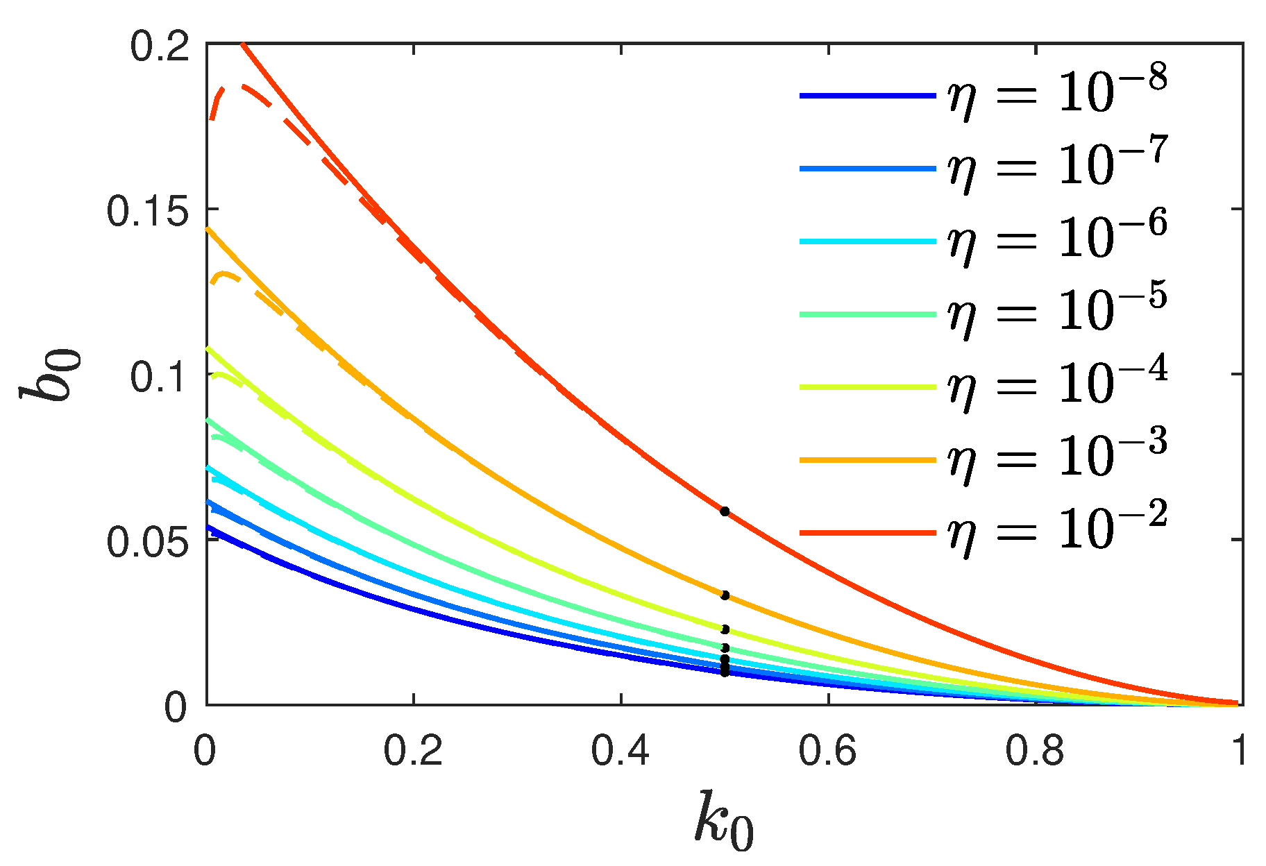
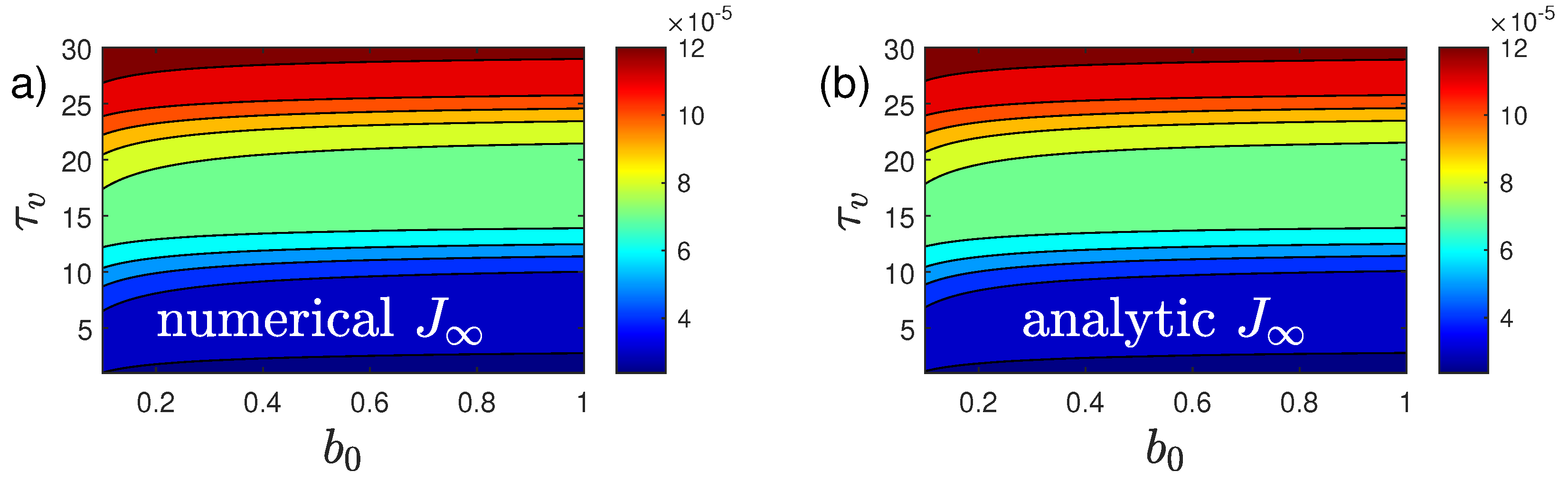
3.3. Properties of the Approximate Solution (22)

The approximate solution (22) is predominantly determined by the reduced time variation of the ratios k ( τ ) and b ( τ ) . For the first and second time derivatives of the solution (22) we obtain
d j d τ = η ( 1 η ) e 0 τ d y b ( y ) k ( τ ) b ( τ ) exp 0 τ d x e 0 x d y b ( y ) k ( x ) b ( x ) ,
d 2 j d τ 2 = η ( 1 η ) [ e 0 τ d y b ( y ) k ( τ ) b ( τ ) ] 2 d k d τ d b d τ b ( τ ) e 0 τ d y b ( y ) × exp 0 τ d x e 0 x d y b ( y ) k ( x ) b ( x ) .
Consequently, extrema of the rate of new infections occur at reduced times τ E determined by
k ( τ E ) + b ( τ E ) = e 0 τ E d y b ( y ) .
As the right-hand side of this Equation is smaller than or equal to unity, no extrema of infections occur for a sum of variations
k ( τ ) + b ( τ ) > 1
greater than unity at all times. As both rates are semi-positive the condition (30) for no extrema in the rate of new infections is fulfilled if either the vaccination rate v ( t ) > a ( t ) is greater than the infection rate and/or the recovery rate μ ( t ) > a ( t ) is greater than the infection rate. For large enough values of k and b, so that k ( τ ) + b ( τ ) > 1 , we have thus shown in Equation (27) that no extrema of the rate of new infections j ( τ ) occur at any reduced time τ 0 . According to Equation (27), then, this rate continually decreases from its original positive initial value j ( τ = 0 ) = η ( 1 η ) to even smaller values at later times. As j ( τ ) = S ( τ ) I ( τ ) and S ( τ ) , as well as I ( τ ) , are originally positive for τ = 0 , they will remain positive. With I ( τ ) and S ( τ ) positive, it is clear from Equations (15) and (16) that R ( τ ) and V ( τ ) are also positively valued at all times.
In the case of reduced time intervals, where
k ( τ ) + b ( τ ) < 1 ,
we obtain
[ d 2 j d τ 2 ] τ E = η ( 1 η ) ( [ d k d τ ] τ E + [ d b d τ ] τ E + b 2 ( τ E ) + b ( τ E ) k ( τ E ) ) × exp 0 τ E d x e 0 x d y b ( y ) k ( x ) b ( x ) ,
so that the extrema are maxima if
[ d k d τ ] τ E + [ d b d τ ] τ E + b 2 ( τ E ) + b ( τ E ) k ( τ E ) > 0
is positive. Alternatively, the extrema are minima if
[ d k d τ ] τ E + [ d b d τ ] τ E + b 2 ( τ E ) + b ( τ E ) k ( τ E ) < 0
is negative. Note that there can be multiple minima and maxima depending on the reduced time variation of the ratios k ( τ ) and b ( τ ) . The extreme values of the rate of new infections are given by
j E ( τ E ) = η ( 1 η ) e 0 τ E d x e 0 x d y b ( y ) k ( x ) b ( x ) .

3.4. Cumulative Fraction

Integrating the rate of new infections (22) provides us with the corresponding cumulative fraction
J ( τ ) = η + η ( 1 η ) 0 τ d z exp 0 z d x ( e 0 x d y b ( y ) k ( x ) b ( x ) ) .
For general reduced time variations k ( τ ) and b ( τ ) , the integral in Equation (36) can be reasonably well approximated and evaluated using the method of steepest descent [34,35] by expanding the argument in the exponential function in Equation (36) to second order in z around its (possible multiple) minimum values τ m
h ( z ) = 0 z d x ( e 0 x d y b ( y ) k ( x ) b ( x ) ) h ( τ m ) + ( z τ m ) 2 h m 2 ,
where
h m = [ d 2 h ( z ) d z 2 ] τ m .
With this expansion, we obtain for the cumulative fraction (36)
J ( τ ) η + η ( 1 η ) m π 2 h m e h ( τ m ) erf h m 2 ( τ τ m ) + erf h m 2 τ m ,
where the sum of m accounts for possible multiple minima and
h ( τ m ) = 0 τ m d x k ( x ) + b ( x ) e 0 x d y b ( y ) , h m = [ d k d τ ] τ m + [ d b d τ ] τ m + b 2 ( τ m ) + b ( τ m ) k ( τ m ) .
For a minimum, the second derivative h m > 0 has to be positive. The minima occur at times given by
k ( τ m ) + b ( τ m ) = e 0 τ m d y b ( y ) ,
and, as discussed before (see Equations (29)–(31)), only for reduced time intervals where the sum k ( τ ) + b ( τ ) < 1 is less than unity.

4. Special Case: Stationary Ratios

We first consider the approximative solutions (19) and (22) in the special case of stationary ratios
k ( τ ) = k 0 , b ( τ ) = b 0 ,
considered before [1]. We readily obtain
V ( τ ) = ( 1 J ) [ 1 e b 0 τ ] ,
and
j ( τ ) = η ( 1 η ) exp 1 e b 0 τ b 0 ( k 0 + b 0 ) τ .
Provided k 0 + b 0 < 1 , the rate of new infections (44) attains its maximum value at the reduced time
τ m = ln ( k 0 + b 0 ) b 0 .
The maximum rate of new infections, then, is
j max = j ( τ m ) = η ( 1 η ) ( k 0 + b 0 ) k 0 + b 0 b 0 e 1 ( k 0 + b 0 ) b 0 .
Equations (45) and (46) agree exactly with Equations (98) and (100) derived before [1].

4.1. Cumulative Fraction
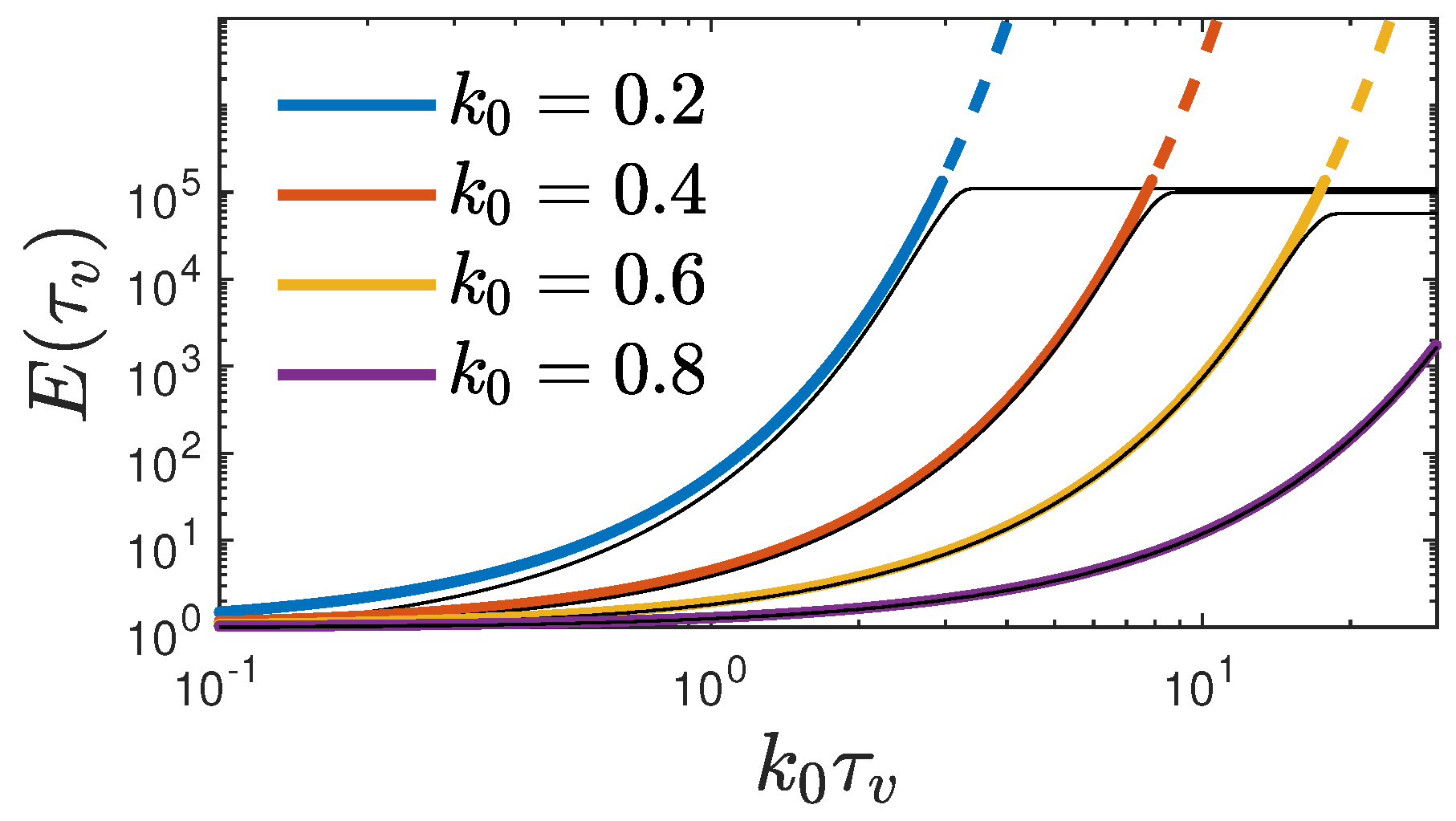
Integrating Equation (44) yields for the cumulative fraction
J ( τ ) = η + η ( 1 η ) H ( τ ) ,
with the integral
H ( τ ) = 0 τ d x exp 1 e b 0 x b 0 ( k 0 + b 0 ) x = b 0 k 0 b 0 e 1 b 0 e b 0 τ b 0 1 b 0 d y y k 0 b 0 e y ,
where we substituted y = e b 0 x / b 0 . The integral (48) can be expressed as the difference of two lower incomplete gamma functions
γ ( s , x ) = 0 x t s 1 e t d t = Γ ( s ) Γ ( s , x ) ,
yielding
H ( τ ) = b 0 k 0 b 0 e 1 b 0 γ 1 + k 0 b 0 , 1 b 0 γ 1 + k 0 b 0 , e b 0 τ b 0 ,
so that the cumulative fraction (47) is given by
J ( τ ) = η + η ( 1 η ) b 0 k 0 b 0 e 1 b 0 γ 1 + k 0 b 0 , 1 b 0 γ 1 + k 0 b 0 , e b 0 τ b 0 .
For infinitely large times, the fraction (51) approaches the final value
J = J ( τ = ) = η + η ( 1 η ) b 0 k 0 b 0 e 1 b 0 γ 1 + k 0 b 0 , 1 b 0 .
Equations (51) and (52) agree exactly with the earlier derived Equations (A10) and (102) of ref. [1], using a different approach.
Because the analytical approximations were derived in the limit J J 1 , for consistency, we have to require J < 1 for the values of k 0 and b 0 for which our approximation holds. In Figure 1, we calculate the required values of k 0 and b 0 fulfilling J < 1 using Equation (52). The required values depend on the initial condition encoded by η , and are located above the line shown in this figure. For sufficiently large k 0 , J < 1 , for any ratio b 0 , while at low recovery to infection ratios k 0 , the vaccination to infection rate must be significant to ensure J < 1 . The regime of b 0 close to zero is numerically difficult to evaluate using Equation (52).

4.2. Limit b 0 1

In the limit of small b 0 1 , we use relation (49) and the asymptotic expansion (Equation 6.5.32 in [36]) of the upper incomplete gamma function for large arguments x 1
Γ ( s , x 1 ) x s 1 e x 1 + s 1 x + ( s 1 ) ( s 2 ) x 2 + ,
to obtain for
γ 1 + k 0 b 0 , 1 b 0 Γ 1 + k 0 b 0 b 0 k 0 b 0 e 1 b 0 [ 1 + k 0 + k 0 ( k 0 1 ) + ] ;
the fraction (52) then becomes
J ( b 0 1 ) η + η ( 1 η ) Γ 1 + k 0 b 0 b 0 k 0 b 0 e 1 b 0 [ 1 + k 0 + k 0 ( k 0 1 ) + ] .
Using Stirling’s formula (Equation 6.1.37 in [36]) for the gamma function Γ ( x + 1 ) 2 π x ( x / e ) x [ 1 + ( 12 x ) 1 ] for large x, Equation (55) becomes,
J ( b 0 1 ) η + η ( 1 η ) 2 π k 0 b 0 k 0 k 0 b 0 e 1 k 0 b 0 1 + b 0 12 k 0 [ 1 + k 0 + k 0 ( k 0 1 ) + ] .
For values of b 0 < k 0 < 1 , the fraction (56) to leading orders is given by
J ( b 0 1 ) η + η ( 1 η ) 2 π k 0 / b 0 e ( 1 k 0 ) / b 0 k 0 k 0 / b 0 1 .
Because one has to require J 1 , or equivalently, ln ( J ) 0 , Equation (57) turns into an inequality for b 0 , which can be written in terms of the principal branch W 0 of Lambert’s W-function, because ( x / b 0 ) ln b 0 = ln y is solved for any x 0 and y by x / W 0 ( x y ) , leading to
b 0 2 ( 1 k 0 + k 0 ln k 0 ) W 0 ( 1 + η ) 2 [ 1 k 0 + k 0 ln ( k 0 ) ] π k 0 η 2 .
This inequality (58) ensures J 1 . Along with the information contained in Equation (52), it is visualized in Figure 1.

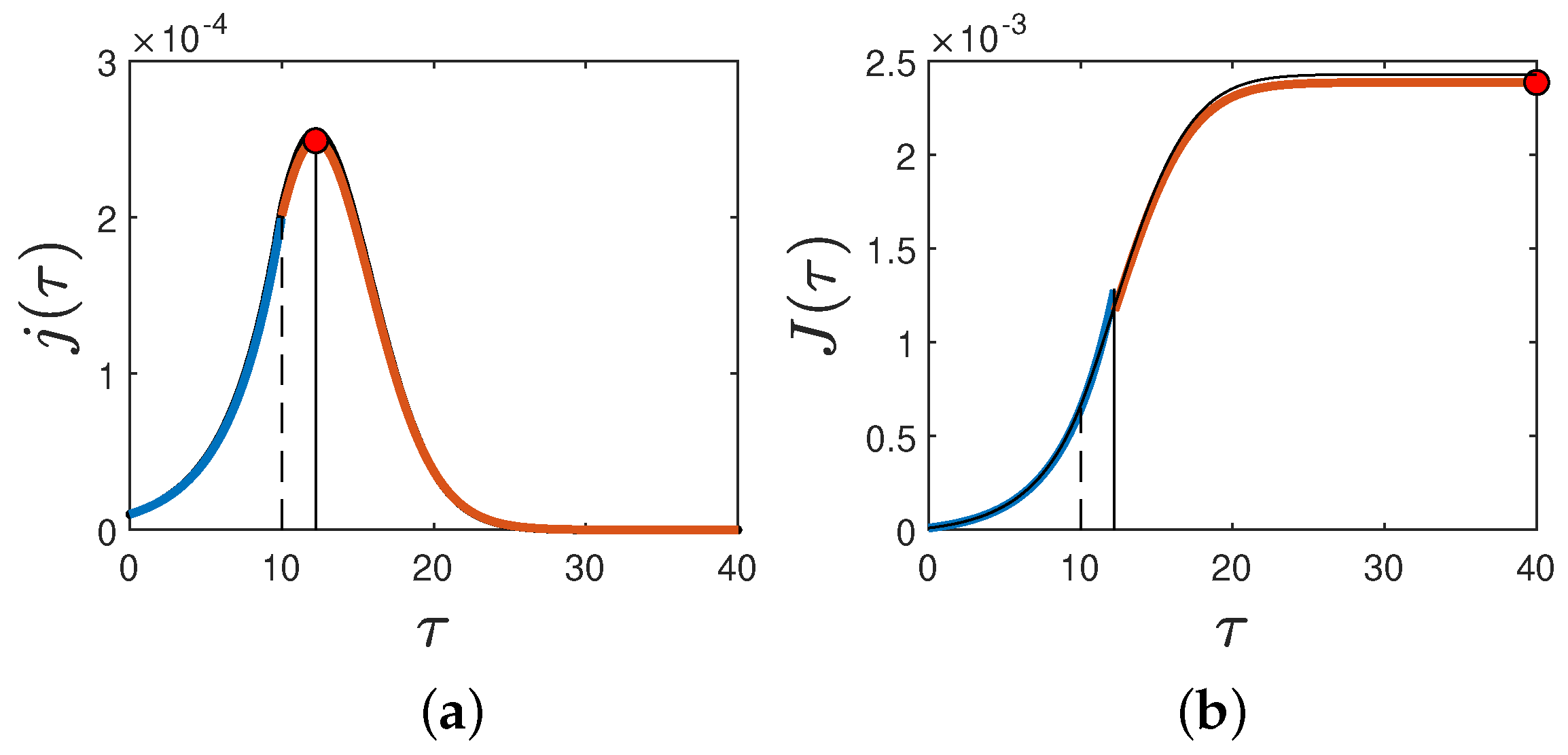
5. Stationary Ratios with Delayed Start of Vaccinations
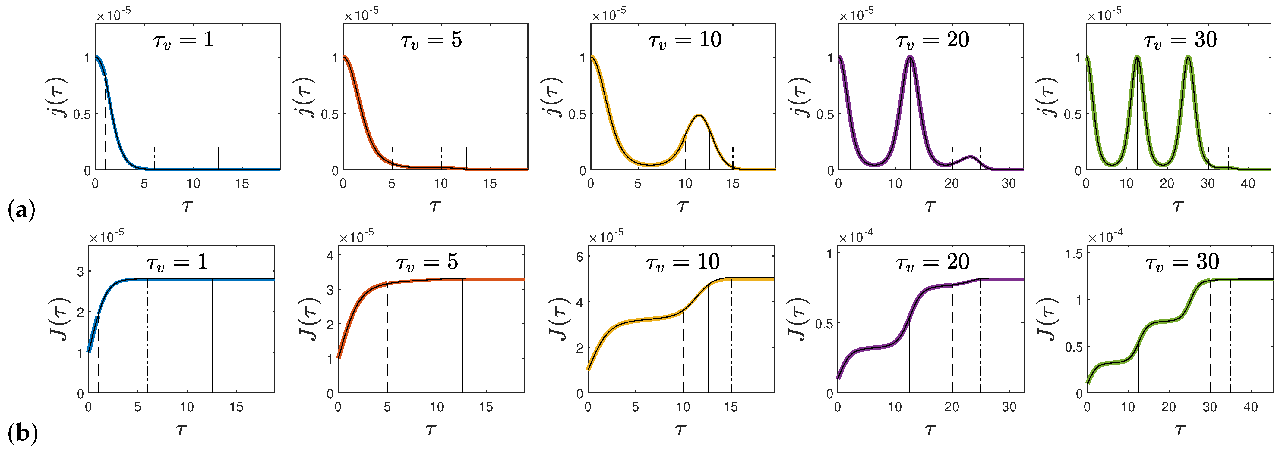
As first new application of our results, we discuss the case of stationary ratio k ( τ ) = k 0 for all reduced times and the influence of a stationary ratio b ( τ ) starting at the delayed reduced time τ v > 0 , i.e.,
k ( τ ) = k 0 , b ( τ ) = b 0 Θ ( τ τ v )
where Θ ( x < 0 ) = 0 and Θ ( x 0 ) = 1 denotes the step function. We then obtain for Equation (19), i.e., in the limit J 1 , V = 0 for τ < τ V and
V ( τ τ v ) = ( 1 J ) [ 1 e b 0 ( τ τ v ) ] .
Likewise, the rate (22) becomes the SIR-rate [27]
j ( 0 τ < τ v ) = η ( 1 η ) e ( 1 k 0 ) τ
at times without vaccination, and
j ( τ τ v ) = η ( 1 η ) exp ( 1 k 0 ) τ v + 1 e b 0 ( τ τ v ) b 0 ( k 0 + b 0 ) ( τ τ v )
at later times. While the SIR-rate (61) is exponentially increasing in reduced time, the rate (62) has a maximum value
j max = j ( τ m ) = η ( 1 η ) exp ( 1 k 0 ) τ v + 1 e b 0 ( τ m τ v ) b 0 ( k 0 + b 0 ) ( τ m τ v ) = η ( 1 η ) ( k 0 + b 0 ) k 0 + b 0 b 0 exp ( 1 k 0 ) τ v + 1 ( k 0 + b 0 ) b 0 ,
provided k 0 + b 0 < 1 , the rate of new infections attains its maximum at the reduced time
τ m = τ v ln ( k 0 + b 0 ) b 0 .
We first note that for τ v = 0 , the rates (62) and (63) correctly reproduce the earlier results (44) and (46). We emphasize that the delayed start of the vaccinations increases both the maximum time of the rate of infections and the maximum rate of new infections. Compared to the case of no delay in the start of vaccinations ( τ v = 0 ), we introduce the enhancement factor for the maximum rate
E ( τ v ) = j max ( τ v ) j max ( τ v = 0 ) = e ( 1 k 0 ) τ v ,
shown in Figure 2, which is independent of the vaccination rate and determined by the values of k 0 and τ v . Apparently, this exponential enhancement solely results from the new infections before the vaccinations start. While the enhancement factor increases exponentially over a wide range of k 0 τ v , in accord with Equation (65), it numerically reaches a plateau as k 0 τ v approaches infinity, whose height increases with decreasing η . This is a clear indication that for large values of the enhancement factor, a regime is reached where J ( τ m ) is no longer much smaller than unity, so that the analytical approximation no longer holds. This explanation is supported by the cumulative fraction at large times (68) (see below) being directly proportional to the enhancement factor (65).
Integrating the rates of new injections (61) and (63) yields for the cumulative fraction
J ( 0 τ < τ v ) = η + η ( 1 η ) 1 k 0 [ e ( 1 k 0 ) τ 1 ] ,
and
J ( τ τ v ) = η + η ( 1 η ) 1 k 0 e ( 1 k 0 ) τ v 1 + η ( 1 η ) b 0 k 0 b 0 e ( 1 k 0 ) τ v + 1 b 0 × γ 1 + k 0 b 0 , 1 b 0 γ 1 + k 0 b 0 , e b 0 ( τ τ v ) b 0 .
For infinitely large times, the fraction (67) approaches the final value J = J ( τ = ) with
J = η + η ( 1 η ) 1 k 0 e ( 1 k 0 ) τ v 1 + η ( 1 η ) b 0 k 0 b 0 e ( 1 k 0 ) τ v + 1 b 0 γ 1 + k 0 b 0 , 1 b 0 = η ( 1 η ) 1 k 0 E ( τ v ) 1 + ( 1 k 0 ) b 0 k 0 b 0 e 1 b 0 γ 1 + k 0 b 0 , 1 b 0 + η ( η k 0 ) 1 k 0 .
An example showing all quantities calculated analytically in this section, along with the numerical solution for a case with J 1 , is given in Figure 3.

6. Oscillating Ratio k with Delayed Vaccinations at Constant Rate b 0

As a second application, we investigate the influence of delayed vaccinations with constant rate on the earlier discussed SIR-application [27] with an oscillating k ratio and delayed vaccination ratio b,
k ( τ ) = 1 + α sin ( β τ ) ,
b ( t ) = b 0 Θ ( τ τ v ) ,
with constant values α and β . As noted before [27] the oscillating ratio (69) represents a series of repeating pandemic outbursts with equal amplitudes in the rate of new infections. We then obtain for Equation (19) V = 0 for τ < τ V and
V ( τ τ v ) = 1 e b 0 ( τ τ v ) .
Likewise, the rate (22) becomes the SIR-rate [27]
j ( 0 τ τ v ) = η ( 1 η ) e α β [ cos ( β τ ) 1 ]
at times without vaccination, and
j ( τ τ v ) = η ( 1 η ) exp α β cos ( β τ ) 1 + 1 e b 0 ( τ τ v ) b 0 ( 1 + b 0 ) ( τ τ v )
at later times. In Figure 4a, we show the rate of new infections (72)–(73) in the case α = 0.8 and β = 0.5 for several values of the starting time of vaccinations τ v and the vaccination rate b 0 = 0.2 . We also compare, in each case, the analytical approximations with the exact rates of new infections from solving the SIRV equations numerically.
For the corresponding cumulative fractions, one finds [27]
J ( τ τ v ) = η + η ( 1 η ) e α β τ I 0 α β + 2 n = 1 I n ( α β ) n β sin ( n β τ )
in terms of an infinite series of the modified Bessel function of the first kind I n ( z ) , and
J ( τ τ v ) = η + η ( 1 η ) e α β { M ( τ ) + τ v I 0 ( α β ) + 2 n = 1 I n ( α β ) n β sin ( n β τ v ) } ,
with the integral
M ( τ ) = τ v τ d x e α β cos ( β x ) ( 1 + b 0 ) ( x τ v ) + 1 e b 0 ( x τ v ) b 0 = 0 τ τ v d y e α β cos [ β ( y + τ v ) ] + g ( y ) ,
where we substituted y = x τ and introduced the function
g ( y ) = 1 e b 0 y b 0 ( 1 + b 0 ) y .
This function (77) has the following asymptotic behaviors for small and large values of b 0 y , i.e.,
g ( y ) b 0 y ( 1 + y 2 ) , for y b 0 1 , 1 b 0 ( 1 + b 0 ) y , for y b 0 1 .
In the following, we therefore approximate the function (77) as g ( y ) g A ( y ) with
g A ( y ) = b 0 y 1 + y 2 Θ b 0 1 y + 1 2 b 0 ( 1 + b 0 ) y ] Θ [ y b 0 1 .
With this approximation, we calculate the integral (76). For values of τ τ v + b 0 1 we obtain
M ( τ τ v b 0 1 ) 0 τ τ v d y e α β cos [ β ( y + τ v ) ] b 0 y ( 1 + y 2 ) = 0 τ τ v d y I 0 α β + 2 n = 1 I n α β cos [ n β ( y + τ v ) ] e b 0 y ( 1 + y 2 ) = π 2 b 0 e b 0 2 I 0 α β erf b 0 2 ( τ τ v + 1 ) erf b 0 2 + 2 n = 1 I n α β e n 2 β 2 2 b 0 W n ( τ ) ,
with
W n ( τ ) = 2 b 0 π e b 0 / 2 e n 2 β 2 2 b 0 0 τ τ v d y cos [ n β ( y + τ v ) ] e b 0 y ( 1 + y 2 ) = e 𝚤 n β ( τ v 1 ) erf b 0 2 ( τ τ v + 1 ) 𝚤 n β 2 b 0 erf b 0 2 𝚤 n β 2 b 0
in terms of error functions with complex arguments. The real part in Equation (81) is calculated in detail in Appendix A, providing
W n ( τ ) = cos [ n β ( τ v 1 ) ] erf b 0 2 ( τ τ v + 1 ) erf b 0 2 + e b 0 2 ( τ τ v + 1 ) 2 π 2 b 0 ( τ τ v + 1 ) cos [ n β ( τ v 1 ) ] cos n β τ e b 0 2 π 2 b 0 cos [ n β ( τ v 1 ) ] cos n β τ v + 2 e b 0 2 ( τ τ v + 1 ) 2 π m = 1 e m 2 4 A n , m ( τ ) m 2 + 2 b 0 ( τ τ v + 1 ) 2 2 e b 0 2 π m = 1 e m 2 4 B n , m ( τ ) m 2 + 2 b 0
with
A n , m ( τ ) = 2 b 0 ( τ τ v + 1 ) cos [ n β ( τ v 1 ) ] cosh m n β 2 b 0 cos n β τ , + m sinh m n β 2 b 0 sin n β τ ,
B n , m ( τ ) = 2 b 0 cos [ n β ( τ v 1 ) ] cosh m n β 2 b 0 cos n β τ v + m sinh m n β 2 b 0 sin n β τ v .
Likewise, in the alternative case τ τ v + b 0 1 , we find
M ( τ τ v b 0 1 ) 0 b 0 1 d y e α β cos [ β ( y + τ v ) ] b 0 y ( 1 + y 2 ) + e 1 2 b 0 b 0 1 τ τ v d y e α β cos [ β ( y + τ v ) ] ( 1 + b 0 ) y = e 1 2 b 0 b 0 1 τ τ v d y I 0 α β + 2 n = 1 I n α β e 𝚤 n β ( y + τ v ) e ( 1 + b 0 ) y + π 2 b 0 e b 0 2 I 0 α β erf b 0 2 ( 1 + b 0 1 ) erf b 0 2 + 2 n = 1 I n α β e n 2 β 2 2 b 0 W n τ v + b 0 1 .
The remaining integrals can be evaluated with the help of
b 0 1 τ τ v d y e ( 1 + b 0 ) y = e 1 + b 0 b 0 e ( 1 + b 0 ) ( τ τ v ) 1 + b 0 ,
and
b 0 1 τ τ v d y e 𝚤 n β ( y + τ v ) ( 1 + b 0 ) y = 1 n 2 β 2 + ( 1 + b 0 ) 2 [ n β sin n β τ ( 1 + b 0 ) cos n β τ e ( 1 + b 0 ) ( τ τ v ) n β sin n β ( τ v + b 0 1 ) ( 1 + b 0 ) cos n β ( τ v + b 0 1 ) e 1 + b 0 b 0 ] .
Consequently, Equation (85) becomes
M ( τ τ v b 0 1 ) π 2 b 0 e b 0 2 I 0 α β erf b 0 2 ( 1 b 0 + 1 ) erf b 0 2 + 2 n = 1 I n α β e n 2 β 2 2 b 0 W n ( τ v + b 0 1 ) + e 1 2 b 0 I 0 α β e 1 + b 0 b 0 e ( 1 + b 0 ) ( τ τ v ) 1 + b 0 + 2 e 1 2 b 0 n = 1 I n ( α β ) n 2 β 2 + ( 1 + b 0 ) 2 × [ n β sin n β τ ( 1 + b 0 ) cos n β τ e ( 1 + b 0 ) ( τ τ v ) n β sin [ n β ( τ v + b 0 1 ) ] ( 1 + b 0 ) cos [ n β ( τ v + b 0 1 ) ] e 1 + b 0 b 0 ] .
For the cumulative fraction (75), we obtain
J ( τ v τ τ v + b 0 1 ) = η + η ( 1 η ) e α β × τ v I 0 α β + M ( τ τ v b 0 1 ) + 2 n = 1 I n ( α β ) n β sin ( n β τ v ) ,
and
J ( τ τ v + b 0 1 ) = η + η ( 1 η ) e α β × τ v I 0 α β + M ( τ τ v b 0 1 ) + 2 n = 1 I n ( α β ) n β sin ( n β τ v ) ,
by inserting Equation (85) and (88), respectively. Hence, the cumulative fraction after infinite time is given by
J = η + η ( 1 η ) e α β { τ v I 0 α β + 2 n = 1 I n ( α β ) n β sin ( n β τ v ) + π 2 b 0 e b 0 2 I 0 α β erf b 0 2 ( 1 + b 0 1 ) erf b 0 2 + 2 n = 1 I n α β e n 2 β 2 2 b 0 W n ( τ v + b 0 1 ) + e 1 2 b 0 I 0 α β e 1 + b 0 b 0 1 + b 0 + 2 e 1 + 2 b 0 2 b 0 n = 1 I n ( α β ) n 2 β 2 + ( 1 + b 0 ) 2 × ( 1 + b 0 ) cos [ n β ( τ v + b 0 1 ) ] n β sin [ n β ( τ v + b 0 1 ) ] } ,
which is compared in Figure 5 with the numerical values. It is sufficient to evaluate the sums up to n = m = 50 ; with this setting, the calculation of a J value lasts only a fraction of a second.

7. Summary and Conclusions

The dynamical equations of the susceptible–infected–recovered/removed–vaccinated (SIRV) epidemic model play an important role in predicting and/or analyzing the temporal evolution of epidemic outbreaks accounting quantitatively for the influence of vaccination campaigns. Additional to the time-dependent infection ( a ( t ) ) and recovery ( μ ( t ) ) rates, regulating the transitions between the compartments S I and I R , respectively, the time-dependent vaccination ( v ( t ) accounts for the transition between the compartments S V of susceptible to vaccinated fractions. Here, apparently for the first time a new approximate analytical solution is derived for arbitrary and different but given temporal dependencies of the infection, recovery and vaccination rates, which is valid for all times after the start of the epidemic for which the cumulative fraction of new infections J ( t ) 1 is much less than unity. As vaccination campaigns automatically reduce the rate of new infections by transferring susceptible persons to vaccinated persons, who then no longer can get infected, the limit J 1 is even better fulfilled than in the SIR-epidemic model, which does not account for vaccinations. The proposed analytical approximation is self-regulating, as the final analytical expression for the cumulative fraction J after infinite time allows us to check the validity of the original assumption J ( t ) J 1 , thus indicating the allowed range of parameter values describing the temporal dependence of the ratios k ( t ) = μ ( t ) / a ( t ) and b ( t ) = v ( t ) / a ( t ) .
The comparison of the analytical approximation for the temporal dependence of the rate of new infections J ˚ ( t ) = a ( t ) S ( t ) I ( t ) , the corresponding cumulative fraction of new infections J ( t ) = J ( t 0 ) + t 0 t d ξ J ˚ ( ξ ) , and the fraction of vaccinated persons V ( t ) , respectively, with the exact numerical solution of the SIRV-equations for two different and interesting applications proves the accuracy of the analytical approach. These two applications were not accessible to analytical treatment before. The considered applications include the cases of stationary ratios with a delayed start of vaccinations, and an oscillating ratio of recovery to infection rate with a delayed vaccination at constant rate. The excellent agreement of the analytical approximations with the exact numerical solution of the SIRV-equations for these two applications proves the accuracy of the analytical approach. In the first case, the effect of a delayed start of vaccinations on the maximum rate of new infections and on the final cumulative fraction of infected persons is quantitatively calculated, demonstrating the importance of an early start of vaccinations during a new epidemic outburst. Moreover, the new analytical approximation agrees favorably well with the earlier obtained analytical approximation [1] for the case of stationary ratios between the recovery to infection rate and the vaccination to infection rate, respectively, implying that the time dependence of the three rates a ( t ) , μ ( t ) , and v ( t ) is the same.
This work has calculated approximately the temporal dependence of the rate of new infections and its corresponding cumulative fraction for a given population size using the SIRV-epidemic model equations for spatially integrated quantities. No attempt has been made to include any spatial spread by diffusion. Future work will be concerned with finding analytical approximations for the more complex set of equations including spatial diffusion [19,37,38,39,40,41,42,43].

Author Contributions

Conceptualization, R.S.; Methodology, R.S. and M.K.; Formal analysis, M.K. and R.S.; Writing—original draft, R.S.; Writing—review & editing, M.K.; Visualization, M.K. All authors have read and agreed to the published version of the manuscript.

Funding

This research received no external funding.

Data Availability Statement

All data are enclosed with this publication.

Conflicts of Interest

The authors declare no conflicts of interest.

Appendix A. Reduction of the Function W n (τ)

In order to reduce the function W n ( τ ) introduced in Equation (81), we use their infinite series representation (Equation 7.1.29 in [36]) for the error function with a complex argument
erf ( X + 𝚤 Y ) = erf ( X ) + e X 2 2 π X [ 1 cos ( 2 X Y ) + 𝚤 sin ( 2 X Y ) ] + 2 π e X 2 m = 1 [ f m ( X , Y ) + 𝚤 g m ( X , Y ) ] e m 2 4 m 2 + 4 X 2 ,
with
f m ( X , Y ) = 2 X 2 X cosh ( m Y ) cos ( 2 X Y ) + m sinh ( m Y ) sin ( 2 X Y ) , g m ( X , Y ) = 2 X cosh ( m Y ) sin ( 2 X Y ) + m sinh ( m Y ) cos ( 2 X Y )
and the properties f m ( X , Y ) = f m ( X , Y ) and g m ( X , Y ) = g m ( X , Y ) . After straightforward but tedious algebra, one obtains for general real values of A, B and C for
e 𝚤 A erf ( C 𝚤 B ) = cos ( A ) erf ( C ) + e C 2 2 π C [ ( 1 cos ( 2 B C ) ) cos A + sin ( 2 B C ) sin A ] + 2 e C 2 π m = 1 e m 2 4 m 2 + 4 C 2 [ f m ( C , B ) cos A + g m ( C , B ) sin A ] = cos ( A ) erf ( C ) + e C 2 2 π C [ cos ( A ) cos ( A + 2 B C ) ] + 2 e C 2 π m = 1 e m 2 4 m 2 + 4 C 2 2 C [ cos ( A ) cosh ( m B ) cos ( A + 2 B C ) ] + m sinh ( m B ) sin ( A + 2 B C ) .
Applying Equation (A3) to the two error functions in Equation (81) then yields Equation (82). For A, B, C equally distributed in the range [ 0 , 10 ] , the first term cos ( A ) erf ( C ) in Equation (A3) contributes on average about 97% to the full expression. This feature can be used to write down a simplified expression for W n ( τ ) .

References

  1. Schlickeiser, R.; Kröger, M. Analytical modeling of the temporal evolution of epidemics outbreaks accounting for vaccinations. Physics 2021, 3, 386–426. [Google Scholar] [CrossRef]
  2. Babaei, N.A.; Özer, T. On exact integrability of a COVID-19 model: SIRV. Math. Meth. Appl. Sci. 2023, 1, 1–18. [Google Scholar]
  3. Rifhat, R.; Teng, Z.; Wang, C. Extinction and persistence of a stochastic SIRV epidemic model with nonlinear incidence rate. Adv. Diff. Eqs. 2021, 2021, 200. [Google Scholar] [CrossRef] [PubMed]
  4. Ameen, I.; Baleanu, D.; Ali, H.M. An efficient algorithm for solving the fractional optimal control of SIRV epidemic model with a combination of vaccination and treatment. Chaos Solit. Fract. 2020, 137, 109892. [Google Scholar] [CrossRef]
  5. Oke, M.; Ogunmiloro, O.M.; Akinwumi, C.T.; Raji, R.A. Mathematical Modeling and Stability Analysis of a SIRV Epidemic Model with Non-linear Force of Infection and Treatment. Commun. Math. Appl. 2019, 10, 717–731. [Google Scholar] [CrossRef]
  6. Liu, X.D.; Wang, W.; Yang, Y.; Hou, B.H.; Olasehinde, T.S.; Feng, N.; Dong, X.P. Nesting the SIRV model with NAR, LSTM and statistical methods to fit and predict COVID-19 epidemic trend in Africa. BMC Public Health 2023, 23, 138. [Google Scholar] [CrossRef]
  7. Mahayana, D. Lyapunov Stability Analysis of COVID-19 SIRV Model. In Proceedings of the 2022 IEEE 18th International Colloquium on Signal Processing & Applications (CSPA 2022), Selangor, Malaysia, 12 May 2022; pp. 287–292. [Google Scholar] [CrossRef]
  8. Petrakova, V.S.; Shaydurov, V.V. SIRV-D Optimal Control Model for COVID-19 Propagation Scenarios. J. Siber. Fed. Univ. Math. Phys. 2023, 16, 87–97. [Google Scholar]
  9. Zhao, Z.; Li, X.; Liu, F.; Jin, R.; Ma, C.; Huang, B.; Wu, A.; Nie, X. Stringent Nonpharmaceutical Interventions Are Crucial for Curbing COVID-19 Transmission in the Course of Vaccination: A Case Study of South and Southeast Asian Countries. Healthcare 2021, 9, 1292. [Google Scholar] [CrossRef]
  10. Smith, D.K.; Lauro, K.; Kelly, D.; Fish, J.; Lintelman, E.; McEwen, D.; Smith, C.; Stecz, M.; Ambagaspitiya, T.D.; Chen, J. Teaching Undergraduate Physical Chemistry Lab with Kinetic Analysis of COVID-19 in the United States. J. Chem. Educ. 2022, 99, 3471–3477. [Google Scholar] [CrossRef]
  11. Huntingford, C.; Rawson, T.; Bonsall, M.B. Optimal COVID-19 Vaccine Sharing Between Two Nations That Also Have Extensive Travel Exchanges. Front. Public Health 2021, 9, 633144. [Google Scholar] [CrossRef]
  12. Marinov, T.T.; Marinova, R.S. Adaptive SIR model with vaccination: Simultaneous identification of rates and functions illustrated with COVID-19. Sci. Rep. 2022, 12, 15688. [Google Scholar] [CrossRef] [PubMed]
  13. Beenstock, M.; Felsenstein, D.; Gdaliahu, M. The joint determination of morbidity and vaccination in the spatiotemporal epidemiology of COVID-19. Spat. Spat.-Tempor. Epidem. 2023, 47, 100621. [Google Scholar] [CrossRef] [PubMed]
  14. Haas, F.; Kröger, M.; Schlickeiser, R. Multi-Hamiltonian structure of the epidemics model accounting for vaccinations and a suitable test for the accuracy of its numerical solvers. J. Phys. A 2022, 55, 225206. [Google Scholar] [CrossRef]
  15. Li, X.; Li, X.; Zhang, Q. Time to extinction and stationary distribution of a stochastic susceptible-infected-recovered-susceptible model with vaccination under Markov switching. Math. Popul. Stud. 2020, 27, 259–274. [Google Scholar] [CrossRef]
  16. Cai, C.R.; Wu, Z.X.; Guan, J.Y. Behavior of susceptible-vaccinated-infected-recovered epidemics with diversity in the infection rate of individuals. Phys. Rev. E 2013, 88, 062805. [Google Scholar] [CrossRef] [PubMed]
  17. Widyaningsih, P.; Nugroho, A.A.; Saputro, D.R.S. Susceptible Infected Recovered Model with Vaccination, Immunity Loss, and Relapse to Study Tuberculosis Transmission in Indonesia. AIP Conf. Proc. 2018, 2014, 020121. [Google Scholar] [CrossRef]
  18. Chapman, J.D.; Evans, N.D. The structural identifiability of susceptible-infective-recovered type epidemic models with incomplete immunity and birth targeted vaccination. Biomed. Signal Process. Control 2009, 4, 278–284. [Google Scholar] [CrossRef]
  19. Wang, J.; Zhang, R.; Kuniya, T. A reaction-diffusion Susceptible-Vaccinated-Infected-Recovered model in a spatially heterogeneous environment with Dirichlet boundary condition. Math. Comp. Simul. 2021, 190, 848–865. [Google Scholar] [CrossRef]
  20. Khader, M.M.; Adel, M. Numerical Treatment of the Fractional Modeling on Susceptible-Infected-Recovered Equations with a Constant Vaccination Rate by Using GEM. Int. J. Nonlin. Sci. Numer. Simul. 2019, 20, 69–75. [Google Scholar] [CrossRef]
  21. Dai, Y.; Zhou, B.; Jiang, D.; Hayat, T. Stationary distribution and density function analysis of stochastic susceptible-vaccinated-infected-recovered (SVIR) epidemic model with vaccination of newborns. Math. Meth. Appl. Sci. 2022, 45, 3401–3416. [Google Scholar] [CrossRef]
  22. Kiouach, D.; El-idrissi, S.E.A.; Sabbar, Y. The impact of Levy noise on the threshold dynamics of a stochastic susceptible-vaccinated-infected-recovered epidemic model with general incidence functions. Math. Meth. Appl. Sci. 2023, 47, 297–317. [Google Scholar] [CrossRef]
  23. Kermack, W.O.; McKendrick, A.G. A contribution to the mathematical theory of epidemics. Proc. R. Soc. A 1927, 115, 700. [Google Scholar] [CrossRef]
  24. Kendall, D.G. Deterministic and stochastic epidemics in closed populations. In Proceedings of the Third Berkeley Symposium on Mathematical Statistics and Probability; University of California Press: Berkeley, CA, USA, 1956; Volume 4, p. 149. [Google Scholar] [CrossRef]
  25. Schlickeiser, R.; Kröger, M. Analytical solution of the SIR-model for the temporal evolution of epidemics: Part B. Semi-time case. J. Phys. A 2021, 54, 175601. [Google Scholar] [CrossRef]
  26. Albidah, A.B. A proposed analytical and numerical treatment for the nonlinear SIR model via a hybrid approach. Mathematics 2023, 11, 2749. [Google Scholar] [CrossRef]
  27. Schlickeiser, R.; Kröger, M. Analytical solution of the SIR-model for the not too late temporal evolution of epidemics for general time-dependent recovery and infection rates. COVID 2023, 3, 1781–1796. [Google Scholar] [CrossRef]
  28. Al-Shbeil, I.; Djenina, N.; Jaradat, A.; Al-Husban, A.; Ouannas, A.; Grassi, G. A New COVID-19 Pandemic Model including the Compartment of Vaccinated Individuals: Global Stability of the Disease-Free Fixed Point. Mathematics 2023, 11, 576. [Google Scholar] [CrossRef]
  29. Sepulveda, G.; Arenas, A.J.; Gonzalez-Parra, G. Mathematical Modeling of COVID-19 Dynamics under Two Vaccination Doses and Delay Effects. Mathematics 2023, 11, 369. [Google Scholar] [CrossRef]
  30. Ul Haq, I.; Ullah, N.; Ali, N.; Nisar, K.S. A New Mathematical Model of COVID-19 with Quarantine and Vaccination. Mathematics 2023, 11, 142. [Google Scholar] [CrossRef]
  31. Liu, X.; Ding, Y. Stability and Numerical Simulations of a New SVIR Model with Two Delays on COVID-19 Booster Vaccination. Mathematics 2022, 10, 1772. [Google Scholar] [CrossRef]
  32. Olivares, A.; Staffetti, E. Optimal control applied to vaccination and testing Ppolicies for COVID-19. Mathematics 2021, 9, 3100. [Google Scholar] [CrossRef]
  33. Schlickeiser, R.; Kröger, M. Key epidemic parameters of the SIRV model determined from past COVID-19 mutant waves. COVID 2023, 3, 592–600. [Google Scholar] [CrossRef]
  34. Morse, P.M.; Feshbach, H. Methods of Theoretical Physics, Part I; McGraw-Hill: New York, NY, USA, 1953. [Google Scholar]
  35. Mathews, J.; Walker, R.L. Mathematical Methods in Physics, 2nd ed.; Benjamin: Menlo Park, CA, USA, 1970. [Google Scholar]
  36. Abramowitz, M.; Stegun, I.A. Handbook of Mathematical Functions; Dover Publications: New York, NY, USA, 1970. [Google Scholar]
  37. Bärwolff, G. A Local and Time Resolution of the COVID-19 Propagation—A Two-Dimensional Approach for Germany Including Diffusion Phenomena to Describe the Spatial Spread of the COVID-19 Pandemic. Physics 2021, 3, 536–548. [Google Scholar] [CrossRef]
  38. Baazeem, A.S.; Nawaz, Y.; Arif, M.S.; Abodayeh, K. Modelling infectious disease dynamics: A robust computational approach for stochastic SIRS with partial immunity and an incidence rate. Mathematics 2023, 11, 4794. [Google Scholar] [CrossRef]
  39. Gribaudo, M.; Iacono, M.; Manini, D. COVID-19 spatial diffusion: A Markovian agent-based model. Mathematics 2021, 9, 485. [Google Scholar] [CrossRef]
  40. Wu, K.; Zhou, K. Traveling waves in a nonlocal dispersal SIR model with standard incidence rate and nonlocal delayed transmission. Mathematics 2019, 7, 641. [Google Scholar] [CrossRef]
  41. Wang, Z.; Guo, Q.; Sun, S.; Xia, C. The impact of awareness diffusion on SIR-like epidemics in multiplex networks. Appl. Math. Comput. 2019, 349, 134–147. [Google Scholar] [CrossRef]
  42. Pastor-Satorras, R.; Castellano, C.; Van Mieghem, P.; Vespignani, A. Epidemic processes in complex networks. Rev. Mod. Phys. 2015, 87, 925–979. [Google Scholar] [CrossRef]
  43. Yang, J.; Liang, S.; Zhang, Y. Travelling waves of a delayed SIR epidemic model with nonlinear incidence rate and spatial diffusion. PLoS ONE 2011, 6, e21128. [Google Scholar] [CrossRef] [PubMed]
Figure 1. Required lower limiting values of b 0 versus k 0 , fulfilling J 1 using Equation (52), for various initial η (solid lines). Within the ( k 0 , b 0 ) region above a certain solid line, J < 1 , while the exact numerical solution features J 1 for any choice of k 0 and b 0 . The regime b 0 1 is numerically difficult to evaluate using Equation (52); beyond k 0 > 1 / 2 (marked by black dots), we use the explicit Equation (58). For k 0 < 1 / 2 , Equation (58) is shown as dashed line, highlighting the region of k 0 where Equation (58) cannot be used.
Mathematics 12 00326 g001
Figure 2. The enhancement factor E ( τ v ) as function of k 0 τ v for various k 0 . Analytical result (65) (colored) compared with the numerical result (black) for b 0 = 0.5 and η = 10 5 . Note the double-logarithmic representation. The dashed parts of the analytic results highlight the regimes for which Equation (65) cannot be used anymore, as J (68) exceeds unity.
Mathematics 12 00326 g002
Figure 3. Example for Section 5 using k 0 = 0.7 , b 0 = 0.1 , τ v = 10 , and η = 10 5 . Numerical solution (solid black curve) for (a) j ( τ ) and (b) J ( τ ) . In (a), the analytical expressions (61) (blue) and (62) (red) had been added. The vertical lines are at τ = τ v (dashed) and τ = τ m (solid), according to Equation (64). The filled red circle corresponds to Equation (63). In (b), the analytical expressions are taken from Equations (66) (blue) and (67) (red), while the red circle marks the analytical expression for J according to Equation (68).
Mathematics 12 00326 g003
Figure 4. (a) Perfect agreement between the analytical solutions (72) and (73) (colored) with the numerical solutions (black) for different values of τ v = 1 , 5 , 10 , 20 , 30 (see figure legends) at α = 0.8 , β = 0.5 , b 0 = 0.2 , and η = 10 5 . For times τ < τ v , the analytical solution is insensitive to τ v , and branches from this curve at τ = τ v . The vertical black lines are at τ = τ v (dashed) and τ = 2 π / β (solid), and τ = τ v + b 0 1 (dot-dashed). (b) Corresponding cumulative J ( τ ) . Numerical solution (black) together with the analytical Equations (74) and (89)–(90) (colored).
Mathematics 12 00326 g004
Figure 5. J as function of b 0 and τ v . Remaining parameters as in Figure 4, i.e., α = 0.8 , β = 0.5 , and η = 10 5 . (a) The numerical result, (b) the analytic result using Equation (91).
Mathematics 12 00326 g005
Table 1. Reported data as of 12 Jan 2024 for final values J and D for several countries with more than P = 10 7 inhabitants. Here, P denotes the total population size, P J and P D the reported total number of infections and fatalities, and J and D the population fractions at the declared end of the pandemics. The table is sorted by ascending J . The data were collected from the following github repository: https://pomber.github.io/covid19/timeseries.json (accessed on 20 December 2023).
Country P / 10 6 PJ / 10 6 J PD / 10 6 D
France64.8839.8670.61450.1660.0026
Korea South51.6330.6160.59300.0340.0007
Portugal10.335.5700.53950.0260.0025
Greece10.755.5480.51630.0350.0032
Netherlands17.028.7130.51200.0240.0014
Australia24.1311.3990.47250.0200.0008
Germany84.0838.2490.45490.1690.0020
Czechia10.564.6180.43730.0420.0040
Italy60.6025.6040.42250.1880.0031
Belgium11.354.7390.41760.0340.0030
United Kingdom65.6424.6590.37570.2210.0034
United States323.13103.8030.32121.1240.0035
Spain46.4413.7700.29650.1190.0026
Chile17.915.1920.28990.0640.0036
Japan126.9933.3200.26240.0730.0006
Argentina43.8510.0450.22910.1300.0030
Turkey79.5117.0430.21430.1010.0013
Brazil207.6537.0760.17850.6990.0034
Romania19.713.3460.16980.0680.0034
Poland37.956.4450.16980.1190.0031
Malaysia31.185.0450.16180.0370.0012
Russia144.3422.0760.15290.3880.0027
Peru31.774.4880.14120.2200.0069
Colombia48.656.3590.13070.1420.0029
Canada36.284.6170.12720.0520.0014
Ukraine45.015.7120.12690.1190.0027
Vietnam92.7011.5270.12430.0430.0005
Bolivia10.891.1940.10970.0220.0021
Cuba11.481.1130.09700.0090.0007
Iran80.277.5720.09430.1450.0018
Guatemala16.581.2380.07470.0200.0012
South Africa55.914.0670.07270.1030.0018
Thailand68.864.7280.06870.0340.0005
Iraq37.202.4660.06630.0250.0007
Ecuador16.381.0570.06450.0360.0022
Dominican Republic10.650.6610.06210.0040.0004
Mexico127.547.4830.05870.3330.0026
Philippines103.324.0770.03950.0660.0006
Morocco35.271.2720.03610.0160.0005
India1420.0044.6910.03150.5310.0004
Indonesia261.126.7380.02580.1610.0006
Saudi Arabia32.280.8300.02570.0100.0003
Venezuela31.570.5520.01750.0060.0002
Algeria40.610.2710.00670.0070.0002
Senegal15.410.0890.00580.0020.0001
Egypt95.690.5160.00540.0250.0003
China1410.004.9040.00350.1010.0001
Disclaimer/Publisher’s Note: The statements, opinions and data contained in all publications are solely those of the individual author(s) and contributor(s) and not of MDPI and/or the editor(s). MDPI and/or the editor(s) disclaim responsibility for any injury to people or property resulting from any ideas, methods, instructions or products referred to in the content.

