Author Contributions
Conceptualization, E.M.-A., S.L.G.-C. and J.B.; methodology, E.M.-A., S.L.G.-C., J.B. and A.L.-F.; software, E.M.-A., S.L.G.-C., J.B. and A.L.-F.; validation, E.M.-A., S.L.G.-C., J.B. and A.L.-F.; formal analysis, E.M.-A., S.L.G.-C. and J.B.; investigation, E.M.-A., S.L.G.-C., J.B. and A.L.-F.; resources, E.M.-A., S.L.G.-C. and A.L.-F.; data curation, E.M.-A., S.L.G.-C. and A.L.-F.; writing—original draft preparation, E.M.-A., S.L.G.-C., J.B. and A.L.-F.; writing—review and editing, E.M.-A., S.L.G.-C., J.B. and A.L.-F.; visualization, E.M.-A., S.L.G.-C. and A.L.-F.; supervision, E.M.-A. and S.L.G.-C.; project administration, E.M.-A. All authors have read and agreed to the published version of the manuscript.
Figure 1.
The 25 examples of the MESSIDOR-2 fundus image dataset.
Figure 1.
The 25 examples of the MESSIDOR-2 fundus image dataset.
Figure 2.
Medicine symbol Caduceus used as watermark.
Figure 2.
Medicine symbol Caduceus used as watermark.
Figure 3.
Proposed hybrid watermarking algorithm.
Figure 3.
Proposed hybrid watermarking algorithm.
Figure 4.
Steered Hermite transform schema.
Figure 4.
Steered Hermite transform schema.
Figure 5.
Inverse Steered Hermite transform schema.
Figure 5.
Inverse Steered Hermite transform schema.
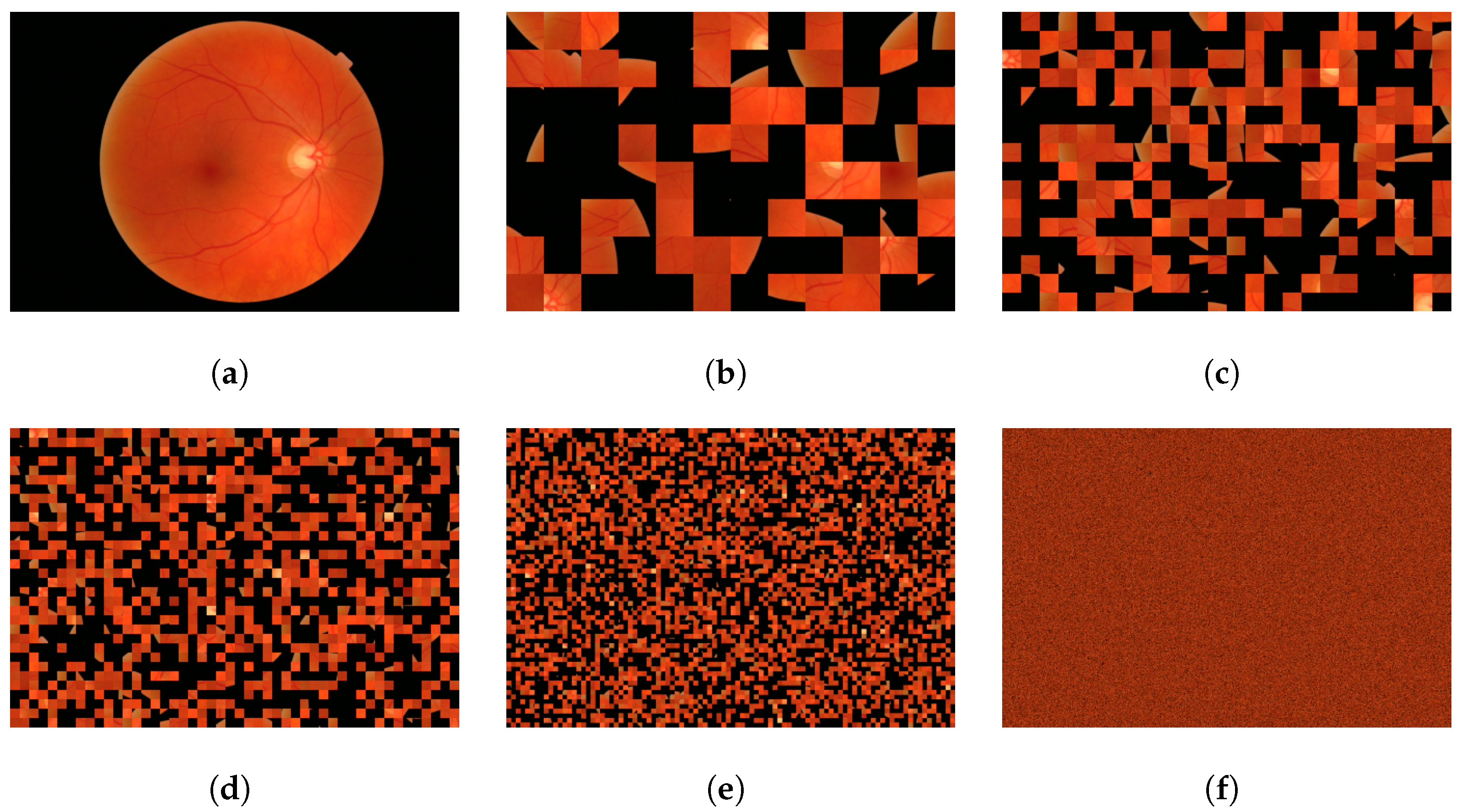
Figure 6.
Examples of the JST a fundus image of pixels, the number of blocks (N) and the size of each one () were varied. (a) Fundus image. (b) and . (c) and . (d) and . (e) and . (f) and . 1,382,400 and .
Figure 6.
Examples of the JST a fundus image of pixels, the number of blocks (N) and the size of each one () were varied. (a) Fundus image. (b) and . (c) and . (d) and . (e) and . (f) and . 1,382,400 and .
Figure 7.
Classic architecture of a convolutional neural network.
Figure 7.
Classic architecture of a convolutional neural network.
Figure 8.
Watermarking insertion schema.
Figure 8.
Watermarking insertion schema.
Figure 9.
(a) Luma component (). (b) Selected Steered Hermite coefficient ().
Figure 9.
(a) Luma component (). (b) Selected Steered Hermite coefficient ().
Figure 10.
Watermarking extraction schema.
Figure 10.
Watermarking extraction schema.
Figure 11.
Sensitivity analysis of the scaling factor , for the ten selected images (A–J images), by varying the scale factor. (a) PSNR values. (b) SSIM values.
Figure 11.
Sensitivity analysis of the scaling factor , for the ten selected images (A–J images), by varying the scale factor. (a) PSNR values. (b) SSIM values.
Figure 12.
Images used for sensitivity analysis of
Figure 11: images (
A–
J).
Figure 12.
Images used for sensitivity analysis of
Figure 11: images (
A–
J).
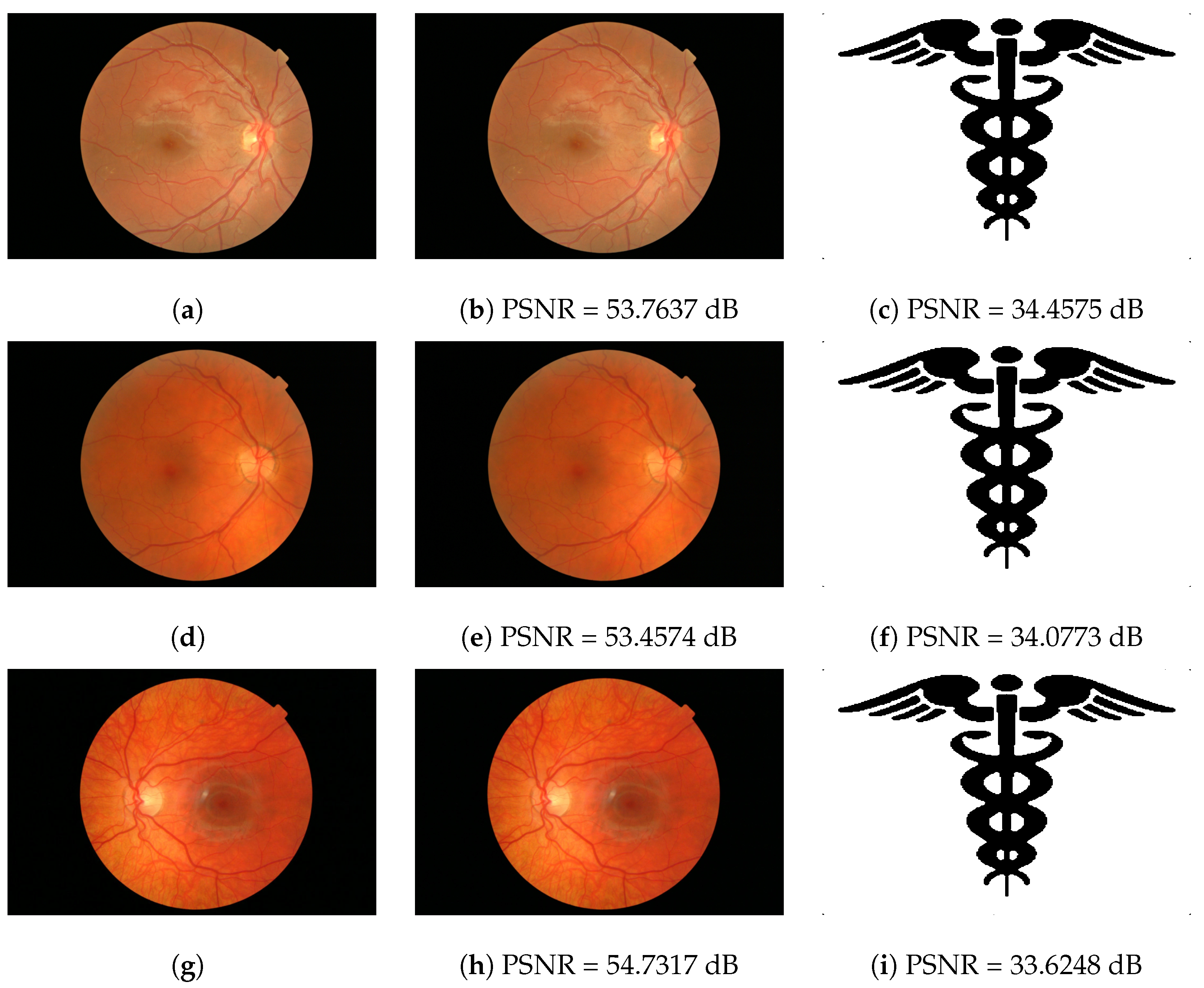
Figure 13.
Best results examples. Original images: (a,d,g). Watermarked images: (b,e,h). Recovery watermark: (c,f,i).
Figure 13.
Best results examples. Original images: (a,d,g). Watermarked images: (b,e,h). Recovery watermark: (c,f,i).
Figure 14.
Worst results examples. Original images: (a,d,g). Watermarked images: (b,e,h). Recovery watermark: (c,f,i).
Figure 14.
Worst results examples. Original images: (a,d,g). Watermarked images: (b,e,h). Recovery watermark: (c,f,i).
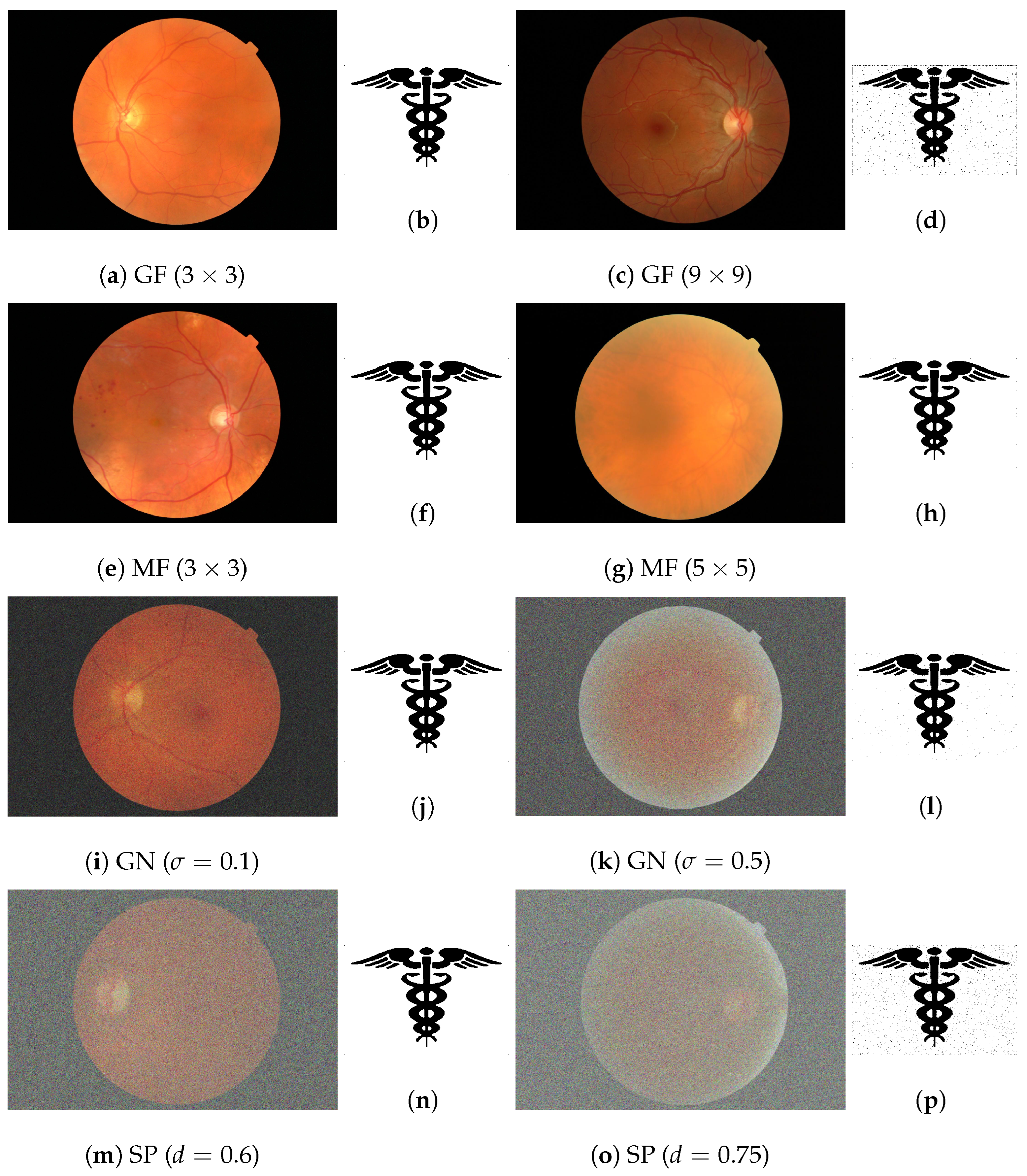
Figure 15.
Results examples of the watermarked and attacked images (GF, MF, GN, SP) and the corresponding extracted watermark, showing satisfying results (b,f,j,n) and those with worse performance (d,h,l,p).
Figure 15.
Results examples of the watermarked and attacked images (GF, MF, GN, SP) and the corresponding extracted watermark, showing satisfying results (b,f,j,n) and those with worse performance (d,h,l,p).
Figure 16.
Results examples of the watermarked and attacked images (CE, EQ, JPEGC, SC) and the corresponding extracted watermark, showing satisfying results (b,f,j,n) and those with worse performance (d,h,l,p).
Figure 16.
Results examples of the watermarked and attacked images (CE, EQ, JPEGC, SC) and the corresponding extracted watermark, showing satisfying results (b,f,j,n) and those with worse performance (d,h,l,p).
Figure 17.
Results examples of the watermarked and attacked images (CE, EQ, JPEGC, SC) and the corresponding extracted watermark, showing satisfying results (b,f,j) and those with worse performance (d,h,l).
Figure 17.
Results examples of the watermarked and attacked images (CE, EQ, JPEGC, SC) and the corresponding extracted watermark, showing satisfying results (b,f,j) and those with worse performance (d,h,l).
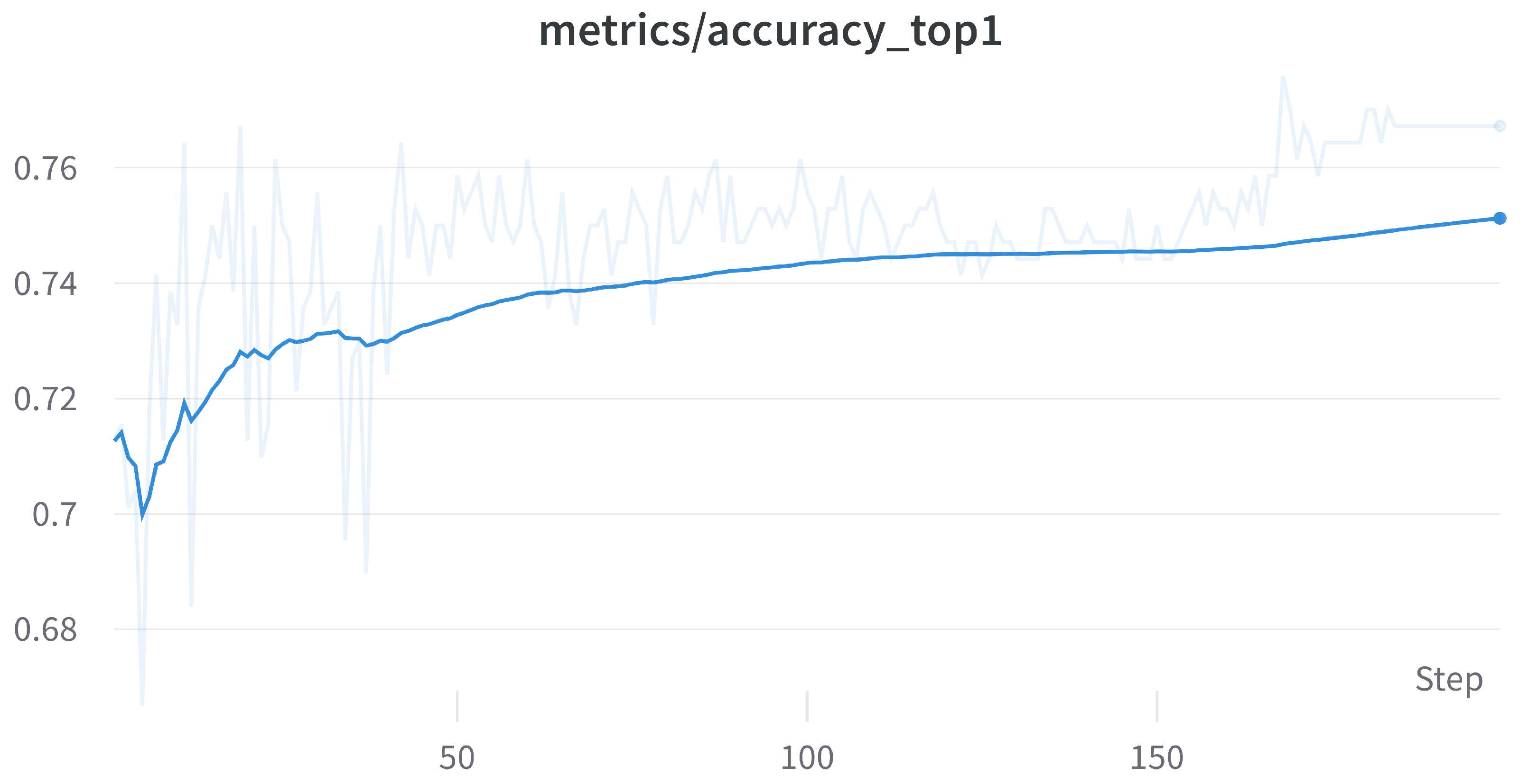
Figure 18.
YOLOv8 top 1 accuracy.
Figure 18.
YOLOv8 top 1 accuracy.
Figure 19.
YoloV8 (a) Original image. (b) Watermarked image. (c) Inference match.
Figure 19.
YoloV8 (a) Original image. (b) Watermarked image. (c) Inference match.
Figure 20.
VGGC16 inference results. (a) VGG16 Accuracy. (b) VGG16 Loss.
Figure 20.
VGGC16 inference results. (a) VGG16 Accuracy. (b) VGG16 Loss.
Figure 21.
VGG16 inference results. (a) Original image. (b) Watermarked image. (c) Inference match.
Figure 21.
VGG16 inference results. (a) Original image. (b) Watermarked image. (c) Inference match.
Figure 22.
InceptionV3 inference results. (a) InceptionV3 Accuracy. (b) InceptionV3 Loss.
Figure 22.
InceptionV3 inference results. (a) InceptionV3 Accuracy. (b) InceptionV3 Loss.
Figure 23.
InceptionV3 inference results. (a) Original image. (b) Watermarked image. (c) Inference mismatch.
Figure 23.
InceptionV3 inference results. (a) Original image. (b) Watermarked image. (c) Inference mismatch.
Figure 24.
InceptionV3 inference results. (a) Original image. (b) Watermarked image. (c) Inference match.
Figure 24.
InceptionV3 inference results. (a) Original image. (b) Watermarked image. (c) Inference match.
Figure 25.
ResNet50 inference results. (a) ResNet50 Accuracy. (b) ResNet50 Loss.
Figure 25.
ResNet50 inference results. (a) ResNet50 Accuracy. (b) ResNet50 Loss.
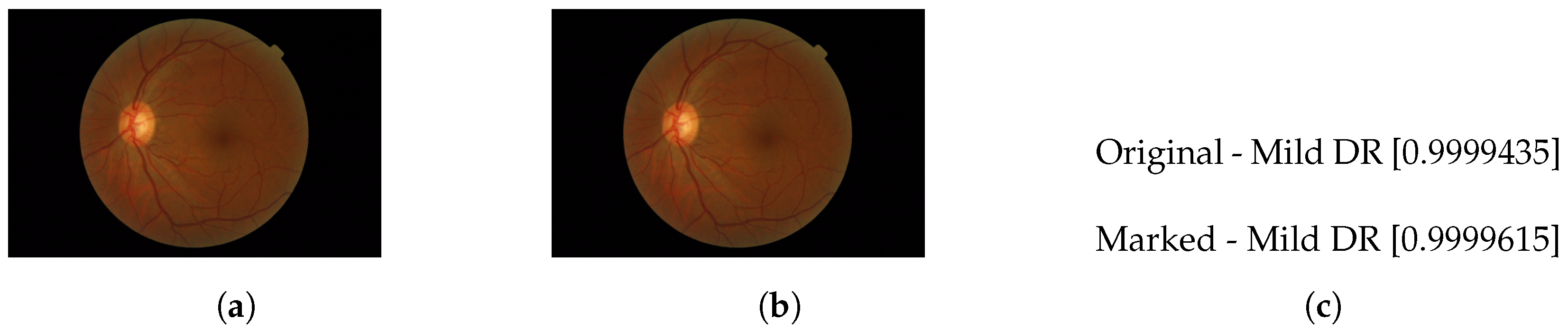
Figure 26.
ResNet50 slight inference results. (a) Original image. (b) Watermarked image. (c) Inference match.
Figure 26.
ResNet50 slight inference results. (a) Original image. (b) Watermarked image. (c) Inference match.
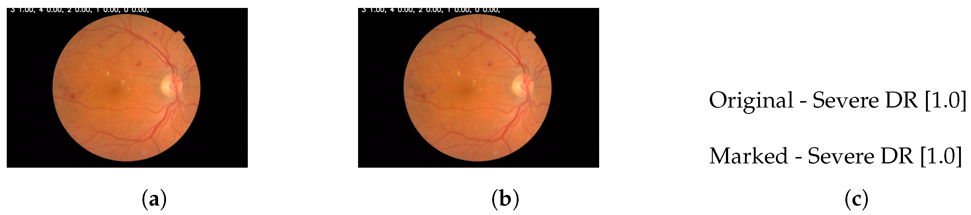
Figure 27.
ResNet50 complete inference results. (a) Original image. (b) Watermarked image. (c) Inference match.
Figure 27.
ResNet50 complete inference results. (a) Original image. (b) Watermarked image. (c) Inference match.
Table 1.
VGG16, ResNet50, and InceptionV3 CNN implementation.
Table 1.
VGG16, ResNet50, and InceptionV3 CNN implementation.
| Network | Number of Layers | Type of Filters | Residual Connections |
|---|
| VGG16 | 16 | | No |
| InceptionV3 | 48 | , , | No |
| ResNet50 | 50 | | Yes |
Table 2.
Average performance metrics for the extracted watermark by varying the scale factor.
Table 2.
Average performance metrics for the extracted watermark by varying the scale factor.
| MSE | PSNR (dB) | NCC | SSIM | MSSIM |
|---|
| 53.50373 | 0.99936 | 0.99330 | 0.99354 |
Table 3.
Average performance metrics using the 1748 fundus images of the MESSIDOR-2 dataset. The insertion section corresponds to the watermarked images and the extraction section to the recovered watermarks.
Table 3.
Average performance metrics using the 1748 fundus images of the MESSIDOR-2 dataset. The insertion section corresponds to the watermarked images and the extraction section to the recovered watermarks.
|
Insertion |
Extraction |
|---|
| MSE | PSNR (dB) | NCC | SSIM | MSSIM | MSE | PSNR (dB) | NCC | SSIM | MSSIM |
| 53.8638 | 0.9993 | 0.9937 | 0.9938 | 0.0007 | 32.0690 | 0.9975 | 0.9937 | 0.9943 |
Table 4.
Definition of the attacks applied and their corresponding parameters.
Table 4.
Definition of the attacks applied and their corresponding parameters.
| Attack Type | Operation Name | Parameter Name | Parameter Value |
|---|
| Image Processing | Gaussian Filter (GF) | Filter size | |
| Median Filter (MF) | Window size | |
| Gaussian Noise (GN) | Variance | |
| Salt and Pepper Noise (SP) | Noise density | d |
| Contrast Enhancement (CE) | Percent saturation | (%) |
| Histogram Equalization (EQ) | Equalization Levels number | |
| JPEG Compression (JPEGC) | Quality Percentage | (%) |
| Image Scaling (SC) | Scaling factor | |
| Geometric | Rotation (ROT) | Rotation angle | (°) |
| Cropping (CROP) | Cropping percentage | (%) |
| Translation (TRAN) | Displaced pixels number | |
Table 5.
Average performance metrics for the extracted watermark using the 1748 fundus images of the MESSIDOR-2 dataset and applying the attacks: GF, MF, GN, and SP.
Table 5.
Average performance metrics for the extracted watermark using the 1748 fundus images of the MESSIDOR-2 dataset and applying the attacks: GF, MF, GN, and SP.
| Attack/Parameter | Parameter Value | MSE | PSNR (dB) | NCC | SSIM | MSSIM |
|---|
| GF/() | | | 32.14117 | 0.99766 | 0.99409 | 0.99457 |
| | 32.06983 | 0.99757 | 0.99383 | 0.99442 |
| | 30.06335 | 0.98959 | 0.96675 | 0.97031 |
| | 18.69012 | 0.71425 | 0.66672 | 0.67248 |
| Average | | 28.24112 | 0.92477 | 0.90535 | 0.90795 |
| MF/() | | | 32.69945 | 0.99808 | 0.99533 | 0.99534 |
| | 32.83169 | 0.99815 | 0.99551 | 0.99550 |
| | 32.78804 | 0.99812 | 0.99545 | 0.99544 |
| | 32.77550 | 0.99800 | 0.99501 | 0.99502 |
| Average | | 32.77367 | 0.99809 | 0.99532 | 0.99532 |
| GN/() | 0.10 | | 31.78001 | 0.99546 | 0.99108 | 0.99191 |
| 0.20 | | 31.59209 | 0.99437 | 0.98949 | 0.99052 |
| 0.40 | | 31.44154 | 0.99417 | 0.98885 | 0.99010 |
| 0.50 | | 31.40980 | 0.99413 | 0.98869 | 0.98998 |
| Average | | 31.55586 | 0.99453 | 0.98952 | 0.99063 |
| SP/(d) | 0.20 | | 31.49094 | 0.99422 | 0.98898 | 0.99016 |
| 0.40 | | 31.43030 | 0.99416 | 0.98877 | 0.99002 |
| 0.60 | | 31.37093 | 0.99407 | 0.98852 | 0.98987 |
| 0.75 | | 31.33329 | 0.99404 | 0.98840 | 0.98979 |
| Average | | 31.40636 | 0.99412 | 0.98867 | 0.98996 |
Table 6.
Average performance metrics for the extracted watermark using the 1748 fundus images of the MESSIDOR-2 dataset and applying the attacks: CE, EQ, JPEG, and SC.
Table 6.
Average performance metrics for the extracted watermark using the 1748 fundus images of the MESSIDOR-2 dataset and applying the attacks: CE, EQ, JPEG, and SC.
| Attack/Parameter | Parameter Value | MSE | PSNR (dB) | NCC | SSIM | MSSIM |
|---|
| CE/() | | | 28.50771 | 0.94652 | 0.91186 | 0.91404 |
| | 29.82147 | 0.95742 | 0.93547 | 0.93700 |
| | 29.35476 | 0.93853 | 0.91139 | 0.91290 |
| | 29.32348 | 0.94157 | 0.90969 | 0.91140 |
| | 29.48612 | 0.94682 | 0.91629 | 0.91815 |
| Average | | 29.29871 | 0.94617 | 0.91694 | 0.91870 |
| EQ/() | 8 | | 32.06528 | 0.99777 | 0.99460 | 0.99466 |
| 32 | | 31.51311 | 0.99747 | 0.99392 | 0.99397 |
| 64 | | 31.41761 | 0.99742 | 0.99378 | 0.99384 |
| 128 | | 31.39045 | 0.99740 | 0.99374 | 0.99380 |
| 256 | | 31.39286 | 0.99740 | 0.99375 | 0.99381 |
| Average | | 31.55586 | 0.99749 | 0.99396 | 0.99402 |
| JPEGC/() | | | 31.39271 | 0.99713 | 0.99252 | 0.99359 |
| | 24.04904 | 0.94505 | 0.88227 | 0.89217 |
| | 19.76781 | 0.83312 | 0.71775 | 0.72688 |
| | 18.57334 | 0.76277 | 0.65339 | 0.66094 |
| | 17.74861 | 0.76366 | 0.64656 | 0.65428 |
| Average | | 22.30630 | 0.86034 | 0.77850 | 0.78557 |
| SC/() | 0.25× | | 0.86967 | 0.00346 | 0.13062 | 0.13400 |
| 0.50× | | 5.24181 | 0.39417 | 0.26875 | 0.27398 |
| 1.50× | | 30.87795 | 0.99413 | 0.98253 | 0.98540 |
| 1.75× | | 30.73933 | 0.99347 | 0.98017 | 0.98318 |
| 2.00× | | 30.09281 | 0.98853 | 0.96374 | 0.96752 |
| Average | | 19.56431 | 0.67475 | 0.66516 | 0.66882 |
Table 7.
Average performance metrics for the extracted watermark using the 1748 fundus images of the MESSIDOR-2 dataset and applying the attacks: ROT, CROP and TRAN.
Table 7.
Average performance metrics for the extracted watermark using the 1748 fundus images of the MESSIDOR-2 dataset and applying the attacks: ROT, CROP and TRAN.
| Attack/Parameter | Parameter Value | MSE | PSNR (dB) | NCC | SSIM | MSSIM |
|---|
| ROT/() | | | 31.91858 | 0.99669 | 0.99097 | 0.99239 |
| | 31.87668 | 0.99649 | 0.99033 | 0.99181 |
| | 31.52496 | 0.99628 | 0.98954 | 0.99103 |
| | 32.11663 | 0.99734 | 0.99301 | 0.99383 |
| | 28.80135 | 0.99527 | 0.98668 | 0.99021 |
| | 32.11481 | 0.99763 | 0.99391 | 0.99438 |
| Average | | 31.39217 | 0.99662 | 0.99074 | 0.99227 |
| CROP/() | | | 33.01504 | 0.99821 | 0.99569 | 0.99565 |
| | 33.00432 | 0.99821 | 0.99567 | 0.99563 |
| | 32.78566 | 0.99812 | 0.99545 | 0.99545 |
| | 28.49738 | 0.99505 | 0.98599 | 0.98966 |
| | 21.70704 | 0.97144 | 0.89202 | 0.90520 |
| | 12.06025 | 0.78417 | 0.47157 | 0.48271 |
| Average | | 26.84495 | 0.95753 | 0.88940 | 0.89405 |
| TRAN/ | (100, 100) px | | 32.88275 | 0.99816 | 0.99555 | 0.99553 |
| (250, 250) px | | 32.89609 | 0.99817 | 0.99558 | 0.99555 |
| (400, 400) px | | 32.93044 | 0.99818 | 0.99560 | 0.99557 |
| (550, 550) px | | 32.99304 | 0.99820 | 0.99566 | 0.99562 |
| Average | | 32.92558 | 0.99818 | 0.99560 | 0.99557 |
Table 8.
Metrics of the extracted watermarks for attacked images from
Figure 15.
Table 8.
Metrics of the extracted watermarks for attacked images from
Figure 15.
| Attack/Parameter | Row (Figure 15) | Parameter Value | PSNR (dB) | NCC | MSSIM |
|---|
| GF/() | 1 (left) | | 34.44387 | 0.99879 | 0.99697 |
| 1 (right) | | 16.77039 | 0.93424 | 0.77541 |
| MF/() | 2 (left) | | 34.40309 | 0.99878 | 0.99694 |
| 2 (right) | | 27.85757 | 0.99449 | 0.98804 |
| GN/() | 3 (left) | 0.1 | 34.37611 | 0.99877 | 0.99692 |
| 3 (right) | 0.5 | 21.46712 | 0.97659 | 0.92703 |
| SP/(d) | 4 (left) | 0.6 | 34.26986 | 0.99874 | 0.99685 |
| 4 (right) | 0.75 | 16.62360 | 0.93240 | 0.72361 |
Table 9.
Metrics of the extracted watermarks for attacked images from
Figure 16.
Table 9.
Metrics of the extracted watermarks for attacked images from
Figure 16.
| Attack/Parameter | Row (Figure 16) | Parameter Value | PSNR (dB) | NCC | MSSIM |
|---|
| CE/() | 1 (left) | | 34.49884 | 0.99881 | 0.99701 |
| 1 (right) | | 12.99699 | 0.85736 | 0.51012 |
| EQ/() | 2 (left) | 128 | 34.40309 | 0.99878 | 0.99694 |
| 2 (right) | 8 | 28.03774 | 0.99472 | 0.98875 |
| JPEGC/() | 3 (left) | | 34.44387 | 0.99879 | 0.99697 |
| 3 (right) | | 13.45755 | 0.86972 | 0.69389 |
| SC/() | 4 (left) | 1.50x | 34.40309 | 0.99878 | 0.99694 |
| 4 (right) | 0.25x | 0.86910 | 0.03747 | 0.14016 |
Table 10.
Metrics of the extracted watermarks for attacked images from
Figure 17.
Table 10.
Metrics of the extracted watermarks for attacked images from
Figure 17.
| Attack/Parameter | Row (Figure 17) | Parameter Value | PSNR (dB) | NCC | MSSIM |
|---|
| ROT/() | 1 (left) | | 34.45754 | 0.99880 | 0.99698 |
| 1 (right) | | 9.70583 | 0.73919 | 0.30531 |
| CROP/() | 2 (left) | | 34.55452 | 0.99882 | 0.99705 |
| 2 (right) | | 24.33087 | 0.98773 | 0.97136 |
| TRAN/() | 3 (left) | px | 34.52659 | 0.99882 | 0.99703 |
| 3 (right) | px | 29.46397 | 0.99619 | 0.99115 |
Table 11.
Comparison values of different algorithms.
Table 11.
Comparison values of different algorithms.
| Watermarking Technique | PSNR (dB) | NCC | SSIM | MSE |
|---|
| Anushikha Singh et al. [9] | 158.4183 | 1.0000 | - | - |
| Zhen Dai et al. [10] | 46.9631 | - | - | - |
| A. George Klington et al. [14] | 54.1572 | - | - | - |
| Ranjana Dwivedi et al. [16] | 46.8600 | - | 0.9914 | - |
| Divyanshu Awasthi et al. [17] | 39.4581 | 0.9957 | 0.9986 | 5.0534 × 10⁻⁵ |
| 67.1475 | 1.0000 | 1.0000 | 8.2033 × 10⁻⁸ |
| Xiyao Liu et al. [18] | 41.2995 | 0.9607 | - | - |
| Muhammad Fachri et al. [19] | 50.5228 | 0.9607 | - | - |
| Payal Garg et al. [22] | 51.7040 | - | - | - |
| Proposed scheme | 53.8638 | 0.9993 | 0.9937 | 4.6976 × 10⁻⁶ |
Table 12.
Comparison of different algorithms about dataset and type of watermarking.
Table 12.
Comparison of different algorithms about dataset and type of watermarking.
| Technique | Image Dataset | Watermark Type | Capacity (Size) |
|---|
| Anushikha Singh et al. [9] | 42 | Digital patient ID | - |
| Zhen Dai et al. [10] | 40 | Binary image | 32 × 32 |
| A. George Klington et al. [14] | 1000 | Fundus image & textual information | 329,960 bits |
| Ranjana Dwivedi et al. [16] | 10 | Color image | 512 × 512 |
| Divyanshu Awasthi et al. [17] | 1 | QR code | 256 × 256 |
| Xiyao Liu et al. [18] | 40 | Hospital logo | 32 × 32 |
| Muhammad Fachri et al. [19] | - | Binary image | 64 × 64 |
| Payal Garg et al. [22] | 1000 | Fingerprints and gait images | - |
| Proposed scheme | 1748 | Binary image | 256 × 256 |
Table 13.
Comparison of different algorithms with our algorithm using Median Filter.
Table 13.
Comparison of different algorithms with our algorithm using Median Filter.
| Technique | Parameter Value | NCC |
|---|
| Ranjana Dwivedi et al. [16] | | |
| |
| Xiyao Liu et al. [18] | | |
| |
| Proposed scheme | | |
| |
| |
Table 14.
Comparison of different algorithms with our algorithm using JPEG Compression.
Table 14.
Comparison of different algorithms with our algorithm using JPEG Compression.
| Technique | Parameter Value | NCC |
|---|
| Ranjana Dwivedi et al. [16] | | |
| Xiyao Liu et al. [18] | | |
| |
| Proposed scheme | | |
| |
| |
Table 15.
Comparison between Xiyao Liu et al. [
18] and our algorithm after Cropping attack.
Table 15.
Comparison between Xiyao Liu et al. [
18] and our algorithm after Cropping attack.
| Technique | Parameter Value | NCC |
|---|
| Xiyao Liu et al. [18] | | |
| |
| Proposed scheme | | |
| |


 ,
, 


