Reversible Data Hiding for Color Images Using Channel Reference Mapping and Adaptive Pixel Prediction

Abstract

Reversible data hiding (RDH) is a technique that embeds secret data into digital media while preserving the integrity of the original media and the secret data. RDH has a wide range of application scenarios in industrial image processing, such as intellectual property protection and data integrity verification. However, with the increasing prevalence of color images in industrial applications, traditional RDH methods for grayscale images are inadequate to meet the requirements of image fidelity. This paper proposes an RDH method for color images based on channel reference mapping (CRM) and adaptive pixel prediction. Initially, the CRM mode for a color image is established based on the pixel variation correlation between the RGB channels. Then, the pixel local complexity context is adaptively selected using the CRM mode. Next, each pixel value is adaptively predicted based on the features and characteristics of adjacent pixels and reference channels, and then data is embedded by expanding the prediction error. Finally, we compare seven existing RDH algorithms on the standard image dataset and the Kodak dataset to validate the advantages of our method. The experimental results demonstrate that our approach achieves average peak signal-to-noise ratio (PSNR) values of 63.61 and 60.53 dB when embedding 20,000 and 40,000 bits of data, respectively. These PSNR values surpass those of other RDH methods. These findings indicate that our method can effectively preserve the visual quality of images even under high embedding capacities.

1. Introduction

Color images constitute a vital component of digital information transmission and storage [1,2,3]. With the rapid advancement of digital technology and the advent of the Industry 4.0 era [4,5,6], the scope of applications for color images continues to expand. They are widely popular in the entertainment sector and play a pivotal role in the industrial domain. Industrial applications typically require high-quality transmission and storage of color images to support decision-making [7], quality control [8], and monitoring production processes [9]. However, safeguarding sensitive information contained within images presents challenges due to the complexity of industrial environments and the stringent requirements for accurate information transmission. Reversible data hiding (RDH) technology has garnered significant attention within information security [10,11,12,13]. This technology’s fundamental attribute lies in its capacity to embed confidential data into images without compromising the original image’s integrity, a crucial feature in industrial applications necessitating the restoration of the original image. In particular, we need to deal with a large amount of color image data in the industrial field, such as images captured by surveillance cameras, product inspection images, and quality control images. These images often contain critical industrial process information and production details, making the utilization of RDH to safeguard sensitive information within industrial images notably valuable. Consequently, this paper proposes a novel RDH method explicitly designed for color images, which enables the concealment of industrial secrets within color images while ensuring both the reversibility of data embedding and extraction and the enhancement of color image fidelity. Furthermore, it safeguards the integrity and security of industrial information.

RDH techniques for grayscale images have been extensively researched, primarily categorizing four categories: methods based on lossless compression [14], histogram shifting (HS) [15], difference expansion (DE) [16], and prediction error expansion (PEE) [17]. Although extensive research and development has been done on RDH for grayscale images, color images are more prevalent in daily life and industrial production. Some researchers have directly applied RDH methods for grayscale images to color images. Nevertheless, this approach neglects the correlation between the three color channels in color images, resulting in a reduced capacity for data embedding. Therefore, in recent years, RDH methods tailored to color images that leverage inter-channel correlations have been proposed. For instance, Yang et al. [18] designed a high-capacity data embedding and extraction method based on the characteristics of color filter array images. In the paper [19], Li et al. utilized an improved predictor to predict each channel of a color image and employed inter-channel correlation for adaptive data embedding, thereby enhancing embedding efficiency. Yao et al. [20] employed guided filtering for prediction in color images and utilized PEE for data embedding, further improving pixel prediction accuracy. The approach proposed by Ou et al. [21] customized effective payload distribution based on the characteristics of each color channel to optimize the process. It also adopted an adaptive embedding strategy to enhance data hiding capacity while minimizing image distortion. Hou et al. [22] introduced a method that maintains grayscale invariance while achieving RDH in color images, ensuring that hidden data can be extracted without affecting the perceived brightness of the image. In the latest research results, Chang et al. [23] dynamically adjusted the embedding mappings of three prediction error histograms based on the inter-channel correlations, thus optimizing embedding performance and image quality. Kong et al. [24] presented an RDH model based on multi-channel difference value ordering. Mao et al. [25] combined the concept of channel unity embedding with pixel value ordering (PVO). Bhatnagar et al. [26] proposed an RDH method for color images based on skewed histograms and cross-channel correlation. Kumar et al. [27] proposed a color image steganography scheme using gray invariant in AMBTC compression domain. In [28], Kumar et al. discussed and reviewed the existing pixel predictors.

While some progress has been made, there remains a need for a deeper exploration of inter-channel correlations in RDH methods for color images to enhance their embedding capacity. The current research exhibits three primary limitations:

• Most methods are extensions of single-channel RDH approaches and need to adequately consider the correlations among color image channels, resulting in limited improvements in embedding capacity.
• Many approaches rely solely on techniques such as prediction error and PVO for data embedding, failing to leverage the untapped potential of other data hiding spaces within color images, such as color space transformation and color quantization.
• The majority of methods employ fixed pixel prediction strategies and parameter settings without dynamic adjustments based on specific image pixel conditions, leading to an imbalance between embedding capacity and pixel distortion.

The preceding analysis indicates that RDH techniques for color images hold significant potential for applications in industrial production and information security. However, existing RDH algorithms for color images still need to be revised, including restricted data embedding capacity, increased image distortion, and underutilized inter-channel correlations. Therefore, our work aims to improve the RDH algorithm’s performance and achieve a balance between the embedding capacity and the visual quality of the images. This goal involves improving the local complexity calculation method and using channel reference mapping and an adaptive pixel prediction strategy. This paper proposes a novel RDH method for color images that addresses these challenges based on channel reference mapping and adaptive pixel prediction. The primary innovations and contributions of our paper are delineated as follows:

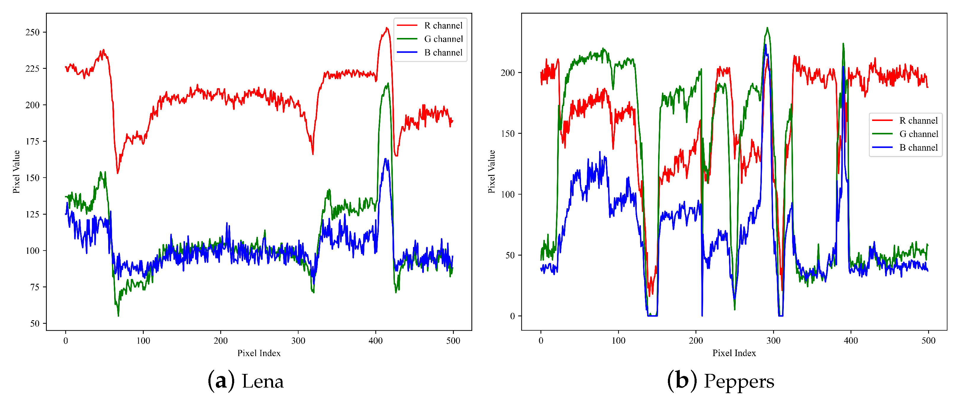
• A novel channel reference mapping (CRM) method is proposed, leveraging trends and correlations among the pixels in the three channels to establish inter-channel reference relationships. These reference relationships are incorporated into pixel-wise local complexity computation and pixel value prediction, thus effectively exploiting the inherent inter-channel connections and reducing pixel distortion during data embedding.
• An adaptive local complexity computation algorithm is proposed. Based on the CRM mode, the current channel’s pixel-wise local complexity computation context is adaptively selected according to the values of reference channel pixels. Adaptive context selection leads to a more accurate assessment of local complexity.
• An adaptive pixel prediction strategy is proposed. By considering each pixel’s neighborhood features and channel characteristics, appropriate predictors and prediction contexts are chosen, thereby enhancing the accuracy of pixel prediction while mitigating image distortion.

The rest of this paper is structured as follows. Section 2 briefly overviews the related works. Section 3 presents the proposed CRM-based RDH method in detail. Section 4 reports the experimental comparison results and analysis that compare our method with other existing algorithms. Section 5 summarizes the paper.

2. Related Work

This section briefly overviews the local complexity method proposed for color images in [21], as detailed in Section 2.1. Additionally, we introduce the pixel prediction method proposed in [19], and specific details can be found in Section 2.2.

2.1. Local Complexity Calculation Method [21]

The selection of pixels for data embedding is a pivotal factor influencing RDH performance, impacting indicators such as data embedding capacity, embedding distortion, and security. While embedding strategies differ between grayscale and color images, opting for low-complexity pixels is generally advantageous as data carriers. This choice has the potential to enhance the overall performance of RDH algorithms. Ou et al. [21] employed inter-channel correlation for computing pixel complexity. The pixel smoothness can be described more accurately by considering the texture similarity among the channels. To reduce pixel distortion, pixels with lower complexity are prioritized for data embedding. $P_x$ and its surrounding eight pixels are illustrated in Figure 1. The complexity calculation for each channel’s pixel $P_x$ is as:

$${\Delta }_x=\left|P_1-P_3\right|+\left|P_2-P_4\right|+\left|P_1+P_2-P_3-P_4\right|+\left|P_2+P_3-P_1-P_4\right|,$$

(1)

where ${\Delta }_x$ represents the complexity of $P_x$. The local complexity calculation methods for the R, G, and B channels are the same. To further enhance the accuracy of pixel complexity calculation, the concepts of the current channel and reference channels are introduced. The current channel is the channel in which the pixel for calculating local complexity is located, and the other two channels are reference channels. With the introduction of reference channels, the local complexity of the current channel pixel $P_x$ is denoted as $LC\left(x\right)$ and is given by:

$$LC\left(x\right)=2{\Delta }_x^c+{\Delta }_x^{r_1}+{\Delta }_x^{r_2},$$

(2)

where ${\Delta }_x^c$ represents the complexity of the current channel, and ${\Delta }_x^{r_1}$ and ${\Delta }_x^{r_2}$ represent the complexities of reference channels. ${\Delta }_x^c$, ${\Delta }_x^{r_1}$, and ${\Delta }_x^{r_2}$ are calculated by Equation (1). Ou et al.’s [21] local complexity calculation method uses a fixed channel ratio, which is not conducive to adapting to different color image features. Therefore, how to adjust the local complexity calculation method adaptively according to the channel correlation of the image is a worthwhile research problem.

2.2. Pixel Prediction Method [19]

Li et al. [19] proposed a pixel prediction method based on the similarity of edge information across channels. They applied different prediction strategies for edge textures with varying levels of complexity. The edge texture, depicted in Figure 1, is accomplished through the pixel’s eight adjacent pixels as:

$$W=\sum _{u=1}^8\left|(P_u^r-P_x^r)/8\right|,$$

(3)

where $P_x^r$ represents the pixel of the reference channel, and $P_u^r$ represents the eight adjacent pixels of $P_x^r$.

To account for the variation of texture complexity in different directions, Li et al. [19] computed the texture complexity for four directions, namely, horizontal, vertical, southeast, and southwest, as:

$$\left\{\begin{array}{c}{W}_h=\left|(P_2^r+P_4^r)/2-P_x^r\right|\hfill \\ W_v=\left|(P_1^r+P_3^r)/2-P_x^r\right|\hfill \\ W_{es}=\left|(P_3^r+P_4^r)/2-P_x^r\right|\hfill \\ W_{ws}=\left|(P_2^r+P_1^r)/2-P_x^r\right|\hfill \end{array}\right..$$

(4)

Let $W_d$ denote the minimum value among $W_h$, $W_v$, $W_{es}$, and $W_{ws}$, expressed as $W_d=min\{W_h,W_v,W_{es},W_{ws}\}$.

A threshold $\theta$ is set to quantify the local complexity of pixels. If $(W-W_d)\le \theta$, the current pixel $P_x^c$ is smooth, and the four pixels adjacent to $P_x^c$ are used for pixel prediction. The prediction formula for pixel ${\widehat{P}}_x^c$ is:

$${\widehat{P}}_x^c=(P_1^c+P_2^c+P_3^c+P_4^c)/4,$$

(5)

where $P_1^c$, $P_2^c$, $P_3^c$, and $P_4^c$ are the four pixels adjacent to $P_x^c$.

If $(W-W_d)>\theta$, the current pixel $P_x^c$ is rough, and the texture in a particular direction may be relatively smooth. In such instances, we use the pixels in the direction with the minimum texture complexity to calculate the pixel prediction value. For example, if $W_d=W_h$, the predicted pixel ${\widehat{P}}_x^c$ is expressed as ${\widehat{P}}_x^c=(P_2^c+P_4^c)/2$. This method determines the pixel prediction value and expands the prediction errors to embed the data. Li et al.’s [19] pixel prediction strategy utilizes the similarity of edge information between channels, but ignores the difference of texture information within channels. Therefore, how to adjust the pixel prediction strategy dynamically according to the channel texture of the image is a worthwhile research problem.

3. Proposed Method

In this section, we provide an extensive exposition of our proposed method, encompassing an overview of the CRM-based RDH framework, the formulation of channel reference mapping, the computation of local complexity, adaptive pixel prediction, and the implementation procedure.

3.1. An Overview of the CRM-Based RDH Framework

The proposed CRM-based RDH framework is composed of two main components: an embedding process and an extraction process. Figure 2 furnishes an illustrative depiction of the CRM-based RDH framework.

On the sender side, we propose a data hiding method based on channel reference mapping (CRM) and adaptive pixel prediction. First, we use the correlation between the three channels of the cover color image I to construct a CRM mode. Next, we calculate the local complexity of each pixel adaptively according to the CRM mode and select the pixels with low complexity for data embedding. After that, we perform adaptive pixel prediction on them and embed data into them. Then, we embed auxiliary information to ensure the reversibility of data hiding. Finally, we combine the pixels of the three channels to obtain the marked color image $I^{\prime }$.

On the receiver side, we reverse the process on the sender side. First, we recover the auxiliary information from the received color image $I^{\prime }$ with hidden data and use it to reconstruct the CRM mode. Then, we calculate the local complexity of each pixel adaptively according to the CRM mode and recover the pixels with low complexity. After that, we use the pixels with low complexity to perform pixel prediction and extract the embedded data. Finally, we recombine the pixels of the three channels to restore the cover color image I.

3.2. Channel Reference Mapping Establishment

The characteristics and texture structures among RGB channels exhibit remarkable similarities, manifested as a fundamental consistency in the pixel value variations across the three channels. This similarity has been extensively validated through a plethora of experiments. We take the images “Lena” and “Peppers” as examples and select 500 pixels from each image. As depicted in Figure 3, the pixel value trends of these pixels show similar monotonicity in the RGB channels.

To analyze the correlation among the RGB channels, we employed the Pearson correlation coefficient as an evaluation metric. The Pearson correlation coefficient is a commonly used statistical method that quantifies the strength and direction of the linear relationship between two variables. Its formula is presented as Equation (6), where $cor(X,Y)$ represents the correlation coefficient between the X and Y channels. The size of the color image is M rows by N columns, with $M\times N$ denoting the total number of pixels in the color image. $X_t$ and $Y_t$ correspond to the pixel values of the X and Y channels at the t-th position, while $\overline{X}$ and $\overline{Y}$ denote the means of all pixels in the X and Y channels, respectively. The value of $cor(X,Y)$ ranges from −1 to 1. Positive values indicate a positive correlation, negative values indicate a negative correlation, and a value of zero indicates no correlation. The larger the absolute value of $cor(X,Y)$, the stronger the correlation between X and Y. The Pearson correlation coefficients between the RGB channels are denoted as $cor(R,G)$, $cor(R,B)$, and $cor(G,B)$, respectively. We represent these three coefficients a set K, specifically $K=\left\{cor\right(R,G),cor(R,B),cor(G,B\left)\right\}$.

$$cor(X,Y)=\frac{{\displaystyle \sum _{t=1}^{M\times N}}(X_t-\overline{X})(Y_t-\overline{Y})}{\sqrt{{\displaystyle \sum _{t=1}^{M\times N}}{(X_t-\overline{X})}^2}\sqrt{{\displaystyle \sum _{t=1}^{M\times N}}{(Y_t-\overline{Y})}^2}}$$

(6)

We denote the maximum and second maximum values in the set K as $K_{max}$ and $K_{smax}$, respectively. Subsequently, we use the functions $chan\left(K_{max}\right)$ and $chan\left(K_{smax}\right)$ to calculate the two channels involved when the correlation coefficients take the values $K_{max}$ and $K_{smax}$, respectively. We express $chan\left(K_{max}\right)$ and $chan\left(K_{smax}\right)$ as

$$\left\{\begin{array}{c}chan\left(K_{max}\right)=(c{h}_1,c{h}_2),s.t.cor(c{h}_1,c{h}_2)=K_{max}\hfill \\ chan\left(K_{smax}\right)=(c{h}_3,c{h}_4),s.t.cor(c{h}_3,c{h}_4)=K_{smax}\hfill \end{array}\right.,$$

(7)

where $c{h}_1$ and $c{h}_2$ represent the two channels involved when the correlation coefficient takes the value $K_{max}$, while $c{h}_3$ and $c{h}_4$ correspond to the two channels associated with $K_{smax}$.

As detailed in

Table 1. Six channel reference mapping modes for color images.

$M_1:\left\{\begin{array}{c}{f}_1\left(R\right)=G\hfill \\ f_2\left(G\right)=B\hfill \\ f_3\left(B\right)=R^{\prime }\hfill \end{array}\right.$	$M_2:\left\{\begin{array}{c}{f}_1\left(R\right)=B\hfill \\ f_2\left(B\right)=G\hfill \\ f_3\left(G\right)=R^{\prime }\hfill \end{array}\right.$	$M_3:\left\{\begin{array}{c}{f}_1\left(G\right)=B\hfill \\ f_2\left(B\right)=R\hfill \\ f_3\left(R\right)=G^{\prime }\hfill \end{array}\right.$
$M_4:\left\{\begin{array}{c}{f}_1\left(G\right)=R\hfill \\ f_2\left(R\right)=B\hfill \\ f_3\left(B\right)=G^{\prime }\hfill \end{array}\right.$	$M_5:\left\{\begin{array}{c}{f}_1\left(B\right)=R\hfill \\ f_2\left(R\right)=G\hfill \\ f_3\left(G\right)=B^{\prime }\hfill \end{array}\right.$	$M_6:\left\{\begin{array}{c}{f}_1\left(B\right)=G\hfill \\ f_2\left(G\right)=R\hfill \\ f_3\left(R\right)=B^{\prime }\hfill \end{array}\right.$

, we can construct six mapping modes between the three channels of a color image, denoted by $M_1$ to $M_6$. Each mapping mode consists of three mapping functions describing the relationship between the current and reference channels. Specifically, the function $f_1\left(X\right)=Y$ represents the first mapping function, indicating the correspondence between the current channel X and the reference channel Y. The function $f_2\left(Y\right)=Z$ represents the second mapping function, illustrating the association between the current channel Y and the reference channel Z. The function $f_3\left(Z\right)=X^{\prime }$ constitutes the third mapping function employed to describe the relationship between the current channel Z and the reference channel $X^{\prime }$. Since data embedding performs in the sequence of channels X, Y, and Z, channel X has already completed data embedding and is denoted as $X^{\prime }$ when data embedding is performed on channel Z.

We describe the process of selecting a suitable CRM mode for a color image from six mapping modes (from $M_1$ to $M_6$) using Algorithm 1. First, we calculate the Pearson correlation coefficients between the three channels according to Equation (6) and store the results in set K. Then, we calculate the maximum value $K_{max}$ and the second largest value $K_{smax}$ in set K. Subsequently, we determine the channels $c{h}_1$ and $c{h}_2$ corresponding to $K_{max}$ and the channels $c{h}_3$ and $c{h}_4$ corresponding to $K_{smax}$ based on Equation (7). After that, we search for the mappings $M_{\delta \left(1\right)}$ and $M_{\delta \left(2\right)}$ that satisfy $f_1\left(c{h}_1\right)=c{h}_2$ or $f_1\left(c{h}_2\right)=c{h}_1$ in the six mapping modes, where $\delta \left(1\right)\in \{1,2,3,4,5,6\}$, $\delta \left(2\right)\in \{1,2,3,4,5,6\}$, and $\delta \left(1\right)\ne \delta \left(2\right)$. Finally, we identify the mapping $M_{\delta \left(3\right)}$ from $M_{\delta \left(1\right)}$ and $M_{\delta \left(2\right)}$ that satisfies either $f_2\left(c{h}_3\right)=c{h}_4$ or $f_2\left(c{h}_4\right)=c{h}_3$, where $\delta \left(3\right)=\delta \left(1\right)$ or $\delta \left(3\right)=\delta \left(2\right)$. Currently, $M_{\delta \left(3\right)}$ becomes the CRM mode established for the cover color image.

Algorithm 1 CRM establishment algorithm

Input:   $R,G,B$: the pixel values of the RGB channels;   $M_1$, $M_2$, $M_3$, $M_4$, $M_5$, $M_6$: six channel reference mapping modes; Output:   $M_{\delta \left(3\right)}$: the established CRM mode; 1: calculate $cor(R,G)$, $cor(R,B)$, and $cor(G,B)$ by Equation (6); 2: $K\leftarrow \left\{cor\right(R,G),cor(R,B),cor(G,B\left)\right\}$; 3: $K_{max}\leftarrow max\left(K\right)$; 4: $K_{smax}\leftarrow max(K-\left\{K_{max}\right\})$; 5: $(c{h}_1,c{h}_2)\leftarrow chan\left(K_{max}\right)$ s.t. $cor(c{h}_1,c{h}_2)=K_{max}$; 6: $(c{h}_3,c{h}_4)\leftarrow chan\left(K_{smax}\right)$ s.t. $cor(c{h}_3,c{h}_4)=K_{smax}$; 7: for each $M_{\alpha }$ in $\{M_1,M_2,M_3,M_4,M_5,M_6\}$ do 8:    if $f_1\left(c{h}_1\right)=c{h}_2$ then 9:      $M_{\delta \left(1\right)}\leftarrow M_{\alpha }$; 10:   end if 11:   if $f_1\left(c{h}_2\right)=c{h}_1$ then 12:     $M_{\delta \left(2\right)}\leftarrow M_{\alpha }$; 13:   end if 14: end for 15: for each $M_{\beta }$ in $\{M_{\delta \left(1\right)},M_{\delta \left(2\right)}\}$ do 16:   if $f_2\left(c{h}_3\right)=c{h}_4\mathrm{or}{f}_2\left(c{h}_4\right)=c{h}_3$ then 17:     $M_{\delta \left(3\right)}\leftarrow M_{\beta }$; 18:   end if 19: end for 20: return $M_{\delta \left(3\right)}$.

3.3. Adaptive Local Complexity Calculation

After obtaining the CRM mode, the data embedding is performed in a per-channel, per-pixel order while scanning the color image from left to right and top to bottom. We employ a method based on local complexity to select suitable embedding pixels, which ensures both image quality and the effectiveness of the concealment. Local complexity is an indicator that measures the extent of change for each pixel, effectively reflecting image details and texture characteristics. A higher local complexity value indicates more information at a particular location, potentially leading to more significant distortions. Therefore, we select pixels with lower local complexity for data embedding to reduce distortion. There are various methods for local complexity calculation, among which the simplest method is to use the difference between the maximum and minimum values in the local complexity context of that pixel. However, this method only considers the four neighboring pixels of the current pixel, disregarding pixel variations over a more extensive range, potentially failing to capture local image features accurately. Hence, we propose an adaptive local complexity computation method leveraging the CRM mode to resolve this limitation, which considers the influence of the current channel and the reference channel over a more extensive range. This method dynamically adjusts parameters according to different image characteristics, leading to a more accurate reflection of pixel complexity.

We denote the current channel being processed as C and the reference channel for the current channel as S. Specifically, the current pixel being processed is $C_{i,j}$, where i and j represent the row and column numbers, respectively. Similarly, $S_{i,j}$ denotes the pixel in the reference channel at row i and column j. To more accurately denote the local complexity of $C_{i,j}$, we extend its local complexity context to a $3\times 3$ pixel block centered at $C_{i,j}$. Likewise, the local complexity context of $S_{i,j}$ in the reference channel is denoted as a $3\times 3$ pixel block centered at $S_{i,j}$. The local complexity contexts of $C_{i,j}$, and $S_{i,j}$ are shown in Figure 4a,b, respectively. The local complexity contexts for $C_{i,j}$ and $S_{i,j}$ are denoted as $NC\left(C_{i,j}\right)$ and $NS\left(S_{i,j}\right)$, and each of them contains 8 pixels, i.e., $NC\left(C_{i,j}\right)$$=\{C_{i-1,j},C_{i,j+1},C_{i+1,j},C_{i,j-1},C_{i-1,j+1},C_{i+1,j+1},C_{i+1,j-1},C_{i-1,j-1}\}$ and $S_{i,j}=\{S_{i-1,j},S_{i,j+1},S_{i+1,j},S_{i,j-1},S_{i-1,j+1},S_{i+1,j+1},S_{i+1,j-1},$$S_{i-1,j-1}\}$. Within $NC\left(C_{i,j}\right)$, the maximum and minimum values are represented as $N{C}_{max}$ and $N{C}_{min}$, while within $NS\left(S_{i,j}\right)$, they are represented as $N{S}_{max}$ and $N{S}_{min}$. We integrate the pixel variation in the local complexity contexts of the current channel and the reference channel and define the local complexity $LC\left(C_{i,j}\right)$ of the current pixel $C_{i,j}$ as

$$LC\left(C_{i,j}\right)={\lambda }_1(N{C}_{max}-N{C}_{min})+{\lambda }_2(N{S}_{max}-N{S}_{min}),$$

(8)

where ${\lambda }_1$ and ${\lambda }_2$ represent the influence weight of the current channel and the reference channel, respectively, ${\lambda }_1\in [0,1]$, ${\lambda }_2\in [0,1]$, and satisfy ${\lambda }_1+{\lambda }_2=1$.

We introduce a parameter named local complexity threshold, denoted by T, to determine whether a pixel is suitable for data embedding. When the local complexity satisfies $LC\left(C_{i,j}\right)\le T$, it indicates that the pixel $C_{i,j}$ has smooth characteristics and is suitable for data embedding. On the contrary, $C_{i,j}$ belongs to the rough category and is unsuitable for data embedding.

3.4. Adaptive Pixel Prediction

We employ the PEE [17] and pixel-based PVO [29] for data embedding. PEE entails an initial prediction of smooth pixels, from which prediction errors are obtained, followed by the subsequent concealment of secret data within these prediction errors. To enhance prediction accuracy and augment the embedding capacity of prediction errors, we propose an adaptive pixel prediction approach. This method automatically selects appropriate prediction contexts based on varying pixel features.

The diamond predictor is a widely used pixel prediction technique to obtain the prediction context of the current pixel $C_{i,j}$, which includes the four adjacent pixels located at the current pixel’s top, bottom, left, and right. However, the prediction range of the diamond predictor is limited and cannot capture a wider range of pixel relationships, especially in complex image scenes. Some pixels may be affected by more distant or complex pixels, but these pixels are not considered, resulting in inaccurate predictions. We propose an adaptive prediction context generation method based on a diamond predictor to address this issue. The diamond prediction context of the current pixel $C_{i,j}$ is denoted as $Rh\left(C_{i,j}\right)$, and the diamond prediction context of the reference pixel $S_{i,j}$ is denoted as $Rh\left(S_{i,j}\right)$. Initially, $Rh\left(C_{i,j}\right)$ includes the four adjacent pixels of the current pixel, i.e., $Rh\left(C_{i,j}\right)=\{C_{i-1,j},C_{i,j+1},C_{i+1,j},C_{i,j-1}\}$, and $Rh\left(S_{i,j}\right)$ includes the adjacent pixels of the reference pixel, i.e., $Rh\left(S_{i,j}\right)=\{S_{i-1,j},S_{i,j+1},S_{i+1,j},S_{i,j-1}\}$. To further expand the scope of the prediction context and consider the consistency of pixel value change trends between the reference channel and the current channel, we utilize the diamond prediction context of the reference channel to assist in the generation of the prediction context of the current channel. We employ $MaxRh\left(S_{i,j}\right)$ and $MinRh\left(S_{i,j}\right)$ to represent the maximum and minimum values in $Rh\left(S_{i,j}\right)$, respectively, and use $Pos\left(MaxRh\left(S_{i,j}\right)\right)$ and $Pos\left(MinRh\left(S_{i,j}\right)\right)$ to represent their positions in the channel. Specifically, $Pos\left(MaxRh\left(S_{i,j}\right)\right)=({\tau }_1,{\tau }_2)$ and $Pos\left(MinRh\left(S_{i,j}\right)\right)=({\tau }_3,{\tau }_4)$. Subsequently, we use the position information of the maximum and minimum values in the reference channel’s diamond prediction context to expand the current channel’s diamond prediction context. This extension is denoted as $Rh\left(C_{{\tau }_1,{\tau }_2}\right)$ and $Rh\left(C_{{\tau }_3,{\tau }_4}\right)$. Afterwards, $PC\left(C_{i,j}\right)$ is utilized to represent the prediction context of the current pixel, defined as

$$PC\left(C_{i,j}\right)=Rh\left(C_{i,j}\right)\cup Rh\left(C_{{\tau }_1,{\tau }_2}\right)\cup Rh\left(C_{{\tau }_3,{\tau }_4}\right)-\left\{C_{i,j}\right\}.$$

(9)

To provide a more detailed explanation of the prediction context generation strategy, we illustrate the generation of $PC\left(C_{i,j}\right)$ as an example in Figure 5. Suppose that the maximum and minimum values in the reference channel $Rh\left(S_{i,j}\right)$ are $S_{i-1,j}$ and $S_{i+1,j}$, respectively, we have $Pos\left(MaxRh\left(S_{i,j}\right)\right)=({\tau }_1,{\tau }_2)=(i-1,j)$ and $Pos\left(MinRh\left(S_{i,j}\right)\right)=({\tau }_3,{\tau }_4)=(i+1,j)$. In this case, $Rh\left(C_{{\tau }_1,{\tau }_2}\right)=Rh\left(C_{i-1,j}\right)$ in the current channel, which includes the pixels $C_{i-2,j}$, $C_{i-1,j-1}$, $C_{i-1,j+1}$, and $C_{i,j}$, i.e., the pixels marked in yellow in Figure 5a. Similarly, $Rh\left(C_{{\tau }_3,{\tau }_4}\right)=Rh\left(C_{i+1,j}\right)$ in the current channel, which includes the pixels $C_{i+1,j-1}$, $C_{i+1,j+1}$, $C_{i+2,j}$, and $C_{i,j}$, i.e., the pixels marked in orange in Figure 5a. In summary, the prediction context $PC\left(C_{i,j}\right)$ for $C_{i,j}$ consists of $C_{i-2,j}$, $C_{i-1,j-1}$, $C_{i-1,j}$, $C_{i-1,j+1}$, $C_{i,j-1}$, $C_{i,j+1}$, $C_{i+1,j-1}$, $C_{i+1,j}$, $C_{i+1,j+1}$, and $C_{i+2,j}$, as indicated by the purple-bordered box in Figure 5b, excluding $C_{i,j}$ itself.

The pixel prediction context, denoted as $PC\left(C_{i,j}\right)$, is a set comprising neighboring pixels surrounding the current pixel, employed for predicting the current pixel. We use $P{C}_{max}$ and $P{C}_{min}$ to denote the maximum and minimum values in the prediction context set, which represent the upper and lower bounds of $C_{i,j}$. To ensure the reversibility of data embedding and extraction, we categorize $C_{i,j}$ into one of four sets as

$$\left\{\begin{array}{c}{Q}_1=\{C_{i,j}\mid P{C}_{max}\ne P{C}_{min},C_{i,j}\ge P{C}_{max}\}\hfill \\ Q_2=\{C_{i,j}\mid P{C}_{max}\ne P{C}_{min},C_{i,j}\le P{C}_{min}\}\hfill \\ Q_3=\{C_{i,j}\mid P{C}_{max}=P{C}_{min},C_{i,j}\le P{C}_{min},P{C}_{min}\ne 254\}\hfill \\ Q_4=\{C_{i,j}\mid P{C}_{max}=P{C}_{min},C_{i,j}\ge P{C}_{max},P{C}_{max}=254\}\hfill \end{array}\right..$$

(10)

If $C_{i,j}$ does not belong to any of these four sets, then the pixel will not be used for data embedding. This approach helps prevent image distortion during data embedding. In such cases, the predicted value of $C_{i,j}$ can be represented by

$${\widehat{C}}_{i,j}=\left\{\begin{array}{cc}P{C}_{max},\hfill & \mathrm{if}{C}_{i,j}\in Q_1\cup Q_4\hfill \\ P{C}_{min},\hfill & \mathrm{if}{C}_{i,j}\in Q_2\cup Q_3\hfill \end{array}\right.,$$

(11)

where ${\widehat{C}}_{i,j}$ represents the predicted value of $C_{i,j}$.

3.5. Data Embedding and Data Extraction

On the sender side, we utilize the reference channel’s pixel information to calculate the current pixel’s local complexity and perform pixel prediction for the smooth pixels. Subsequently, we expand the prediction error to embed secret data. The prediction error of $C_{i,j}$, denoted as $e_{i,j}$, can be calculated as

$$e_{i,j}=C_{i,j}-{\widehat{C}}_{i,j}.$$

(12)

If $C_{i,j}$ falls within $Q_1$ or $Q_4$, we observe that $e_{i,j}\ge 0$. If $C_{i,j}$ falls within $Q_2$ or $Q_3$, then we have $e_{i,j}\le 0$. We select the prediction errors with the highest distribution in the prediction error histograms for expansion to maximize the embedding capacity of the cover color image. Specifically, we use the bins with $e_{i,j}=0$ for data embedding, and the prediction error expansion is defined as

$${\tilde{e}}_{i,j}=\left\{\begin{array}{cc}{e}_{i,j}+b,\hfill & \mathrm{if}{C}_{i,j}\in Q_1\cup Q_4\mathrm{and}{e}_{i,j}=0\hfill \\ e_{i,j}+1,\hfill & \mathrm{if}{C}_{i,j}\in Q_1\cup Q_4\mathrm{and}{e}_{i,j}>0\hfill \\ e_{i,j}-b,\hfill & \mathrm{if}{C}_{i,j}\in Q_2\cup Q_3\mathrm{and}{e}_{i,j}=0\hfill \\ e_{i,j}-1,\hfill & \mathrm{if}{C}_{i,j}\in Q_2\cup Q_3\mathrm{and}{e}_{i,j}<0\hfill \end{array}\right.,$$

(13)

where ${\tilde{e}}_{i,j}$ represents the expanded prediction error and b denotes the secret data to be embedded, with $b\in \{0,1\}$. Finally, the marked pixel ${\tilde{C}}_{i,j}$ is calculated as

$${\tilde{C}}_{i,j}={\widehat{C}}_{i,j}+{\tilde{e}}_{i,j}.$$

(14)

The process of data extraction is the reverse of data embedding. On the receiving end, we utilize the same CRM mode as data embedding to extract secret data pixel by pixel and channel by channel. The channel order for extraction is the reverse of that used for embedding. Similarly, data extraction for each channel follows a bottom-to-top and right-to-left sequence. For each pixel, we initially calculate the local complexity of the current channel’s pixels by leveraging the reference channel, following the same approach as used in embedding. Subsequently, we adaptively compute the prediction context $PC\left({\tilde{C}}_{i,j}\right)$ for smooth pixels, with ${PC}_{max}^{\prime }$ and ${PC}_{min}^{\prime }$ represent the maximum and minimum values within $PC\left({\tilde{C}}_{i,j}\right)$. Afterwards, we categorize ${\tilde{C}}_{i,j}$ into one of the following sets:

$$\left\{\begin{array}{c}{Q}_1=\{{\tilde{C}}_{i,j}\mid {PC}_{max}^{\prime }\ne {PC}_{min}^{\prime },{\tilde{C}}_{i,j}\ge {PC}_{max}^{\prime }\}\hfill \\ Q_2=\{{\tilde{C}}_{i,j}\mid {PC}_{max}^{\prime }\ne {PC}_{min}^{\prime },{\tilde{C}}_{i,j}\le {PC}_{min}^{\prime }\}\hfill \\ Q_3=\{{\tilde{C}}_{i,j}\mid {PC}_{max}^{\prime }={PC}_{min}^{\prime },{\tilde{C}}_{i,j}\le {PC}_{min}^{\prime },{PC}_{min}^{\prime }\ne 254\}\hfill \\ Q_4=\{{\tilde{C}}_{i,j}\mid {PC}_{max}^{\prime }={PC}_{min}^{\prime },{\tilde{C}}_{i,j}\ge {PC}_{max}^{\prime },{PC}_{max}^{\prime }=254\}\hfill \end{array}\right..$$

(15)

Consequently, we predict the pixel value and derive the predicted pixel value ${\widehat{C}}_{i,j}$ as

$${\widehat{C}}_{i,j}=\left\{\begin{array}{cc}{PC}_{max}^{\prime },\hfill & \mathrm{if}{\tilde{C}}_{i,j}\in Q_1\cup Q_4\hfill \\ {PC}_{min}^{\prime },\hfill & \mathrm{if}{\tilde{C}}_{i,j}\in Q_2\cup Q_3\hfill \end{array}\right..$$

(16)

The subsequent step entails the computation of the expanded prediction error, denoted as ${\tilde{e}}_{i,j}$, and it is formulated as

$${\tilde{e}}_{i,j}={\tilde{C}}_{i,j}-{\widehat{C}}_{i,j}.$$

(17)

Currently, the original prediction error, represented as $e_{i,j}$, can be restored using

$$e_{i,j}=\left\{\begin{array}{cc}{\tilde{e}}_{i,j},\hfill & \mathrm{if}{\tilde{e}}_{i,j}=0\hfill \\ {\tilde{e}}_{i,j}-1,\hfill & \mathrm{if}{\tilde{e}}_{i,j}>0\hfill \\ {\tilde{e}}_{i,j}+1,\hfill & \mathrm{if}{\tilde{e}}_{i,j}<0\hfill \end{array}\right..$$

(18)

Simultaneously, the secret data $b=0$ is extracted when ${\tilde{e}}_{i,j}=0$ and $b=1$ when ${\tilde{e}}_{i,j}\in \{0,1\}$. Finally, the original pixel value $C_{i,j}$ is restored to

$$C_{i,j}={\widehat{C}}_{i,j}+e_{i,j}.$$

(19)

3.6. Implementation of the Proposed CRM-Based Method

At the sending end, the data embedding process is specified as follows.

(1) Pretreatment and LM generation. To avoid the pixel value overflow and underflow caused by data embedding, we design three location maps ($L{M}_r$, $L{M}_g$, and $L{M}_b$), corresponding to the red, green, and blue channels of the cover color image, respectively. Each location map shares the same dimensions as the cover color image, i.e., $M\times N$. Initially, all elements of the location maps are set to 0. Then, we perform pixel-by-pixel preprocessing on each channel of the cover color image, changing the pixel values from 255 to 254, changing the pixel values from 0 to 1, and setting the elements of the corresponding location map to 1.

(2) Payload embedding. After obtaining the location maps ($L{M}_r$, $L{M}_g$, and $L{M}_b$) for three channels, we employ arithmetic coding algorithms to compress these maps. The lengths of the compressed location maps are denoted as $L_{cr}$, $L_{cg}$, and $L_{cb}$, and their total length is represented as $L_{clm}$, where $L_{clm}=L_{cr}+L_{cg}+L_{cb}$. The payload consists of two parts, the first part is the secret data, and the second part is a binary sequence derived from the least significant bits (LSBs) of the first (150 + $L_{clm}$) pixels from the top and bottom two rows of each channel in the cover color image. According to the established CRM mode $M_{\delta \left(3\right)}$, we embed the payload into the cover color image in a channel-by-channel and pixel-by-pixel manner.

(3) Auxiliary information and compressed LM embedding. After completing the embedding of the payload, we use the LSB replacement method to embed the auxiliary information into the first 150 pixels of the first row of the red channel of the cover color image. The auxiliary information consists of the following parts: $L_{cr}$ (20 bits), $L_{cg}$ (20 bits), $L_{cb}$ (20 bits), $M_{\delta \left(3\right)}$ (10 bits), T (8 bits), and the positions where the payload embedding ends in the three channels, denoted by $(R_r,R_c)$, $(G_r,G_c)$, and $(B_r,B_c)$, respectively. Each of the six position information occupies 12 bits, totaling 72 bits. Following the auxiliary information, we embed the compressed $LM$ into the cover color image.

At the receiving end, the processing steps for data extraction are detailed below.

(1) Auxiliary information and compressed LM extraction. Initially, we extract auxiliary information from the red channel of the marked color image by the LSB replacement method, which is located in the first row’s first 150 pixels. Then, we utilize the extracted $L_{c}r$, $L_{cg}$, and $L_{cb}$ to extract the compressed $LM$.

(2) Payload extraction and pixel recovery. We employ arithmetic coding algorithms to decompress $LM$. Following the CRM mode $M_{\delta \left(3\right)}$, we extract the payload pixel by pixel in reverse order from the point where data embedding concluded. Simultaneously, we restore the original cover pixels.

(3) Image recovery. We separately restore the secret data and the LSBs of the original pixels from the extracted payload. Additionally, we perform LSB replacement for the first 150 pixels of the red channel. This process ultimately achieves the full restoration of the original color image and the secret data.

4. Experimental Results and Analysis

In this section, we evaluate the performance of the proposed CRM-based RDH method on various color images. First, we verify the method’s effectiveness on six classic color images. Then, we perform performance tests on the method using the Kodak dataset. Finally, we analyze and summarize the performance of the method.

4.1. Color Image Datasets

We use the USC-SIPI (http://sipi.usc.edu/database/database.php?volume=misc (accessed on 20 December 2023)) and Kodak (http://r0k.us/graphics/kodak/ (accessed on 20 December 2023)) datasets as experimental images to evaluate the algorithm’s performance. We compare the proposed algorithm with the state-of-the-art algorithms, measuring image fidelity using peak signal-to-noise ratio (PSNR) values. Figure 6 illustrates six classic color images of size $512\times 512$ from the USC-SIPI dataset: Lena, Airplane, Lake, Peppers, Splash, and House. The Kodak dataset contains 24 color images of size $512\times 768$ or $768\times 512$, on which we test the algorithm’s performance. The secret data used in the experiments is a bit sequence composed of 0 and 1 generated by a random function. We run our method and the compared methods on a PC equipped with Intel Core i7-9700K CPU (Intel Corporation, Santa Clara, CA, USA), 16 GB memory, and Windows 10 operating system, using MATLAB R2020a environment.

4.2. Performance Comparison on Classic Color Images

To assess the performance of CDPP [21], GF-CI [20], GI-CI [22], BRG-EP [30], ATDHM [23], OPC-PVO [31], and the proposed CRM-based RDH method in terms of image fidelity, we performed a set of comparison experiments on six classic USC-SIPI images shown in Figure 6. We utilize the PSNR in decibels (dB) to gauge the fidelity between the cover color image and the marked color image. A higher PSNR value signifies higher similarity and superior image quality. We embed 20,000 and 40,000 bits of secret data in each of the six images shown in Figure 6, respectively, and present the PSNR values after data embedding in

Table 2. Comparisons in terms of PSNR (dB) on six classic color images with a payload of 20,000 bits.

Image	CDPP	GF-CI	GI-CI	BRG-EP	ATDHM	OPC-PVO	Proposed
Lena	60.58	62.15	48.85	51.08	61.58	62.33	62.62
Airplane	64.72	65.36	55.58	60.49	65.48	64.71	65.74
Lake	60.34	62.68	50.58	57.29	62.72	62.76	62.92
Peppers	57.10	58.23	46.12	50.54	57.79	62.50	59.91
Splash	62.28	62.15	54.96	58.93	63.21	64.36	63.50
House	66.01	65.96	58.46	64.10	66.72	64.05	66.97
Average	61.84	62.76	52.43	57.07	62.92	63.45	63.61

and

Table 3. Comparisons in terms of PSNR (dB) on six classic color images with a payload of 40,000 bits.

Image	CDPP	GF-CI	GI-CI	BRG-EP	ATDHM	OPC-PVO	Proposed
Lena	57.85	59.24	46.14	48.23	58.96	59.18	59.31
Airplane	61.87	62.35	53.05	57.18	62.54	62.34	62.58
Lake	56.46	58.65	46.47	52.34	58.03	58.72	58.89
Peppers	54.64	55.66	43.45	47.68	55.44	58.27	56.87
Splash	60.15	60.52	52.14	55.89	60.18	61.82	61.16
House	63.29	63.24	54.28	60.03	64.09	61.75	64.35
Average	59.04	59.94	49.26	53.56	59.87	60.35	60.53

. The results from Table 2 and Table 3 demonstrate that our proposed method achieves higher image quality on most images with the same payload. Our method exhibits superior image quality compared to the GI-CI and BRG-EP. For example, when embedding 20,000 bits, our method yields an average PSNR improvement of 11.18 dB over GI-CI and 6.54 dB over BRG-EP across the six images. This superiority is attributed to our method’s comprehensive exploitation of the relationships between the RGB channels and the establishment of appropriate reference relationships, which excel in local complexity computation and pixel prediction. However, the recently proposed OPC-PVO method could perform better than our method on the Peppers and Splash images. Our method adopts pixel-by-pixel data embedding after establishing the channel reference relationship. In contrast, the OPC-PVO method adopts a pixel-block embedding method, which controls the size of the pixel block to ensure higher pixel quality.

To further validate the superiority of our proposed method in terms of image fidelity, we conduct an experiment in which we plot the PSNR values against the amount of data embedded. The experiment starts with 20,000 bits, increasing in increments of 2000 bits, as depicted in Figure 7. This figure illustrates the trend of PSNR values with respect to data embedding quantities. Our method consistently maintains a high PSNR value even as the volume of embedded data increases. This observation implies that our method effectively preserves image quality and mitigates the distortion resulting from data embedding. Our method outperforms other methods on six classic USC-SIPI images. For example, when we embed 30,000 bits of data into the Lena image, our method achieves a PSNR of 60.82 dB, significantly surpassing the performance of competing methods. Specifically, it outperforms CDPP [21], GF-CI [20], and ATDHM [23] by 1.74, 0.27, and 0.69 dB, respectively. These results underscore the efficacy of our approach in leveraging inter-channel correlations within the RGB color space and intra-channel pixel-level correlations. Ultimately, this approach enhances both image quality and data-hiding capabilities. The aforementioned experiments contribute to a more comprehensive understanding of the proposed algorithm’s performance under varying data loads. Additionally, they assist in determining the optimal data embedding capacity for achieving the highest image fidelity. These findings will further substantiate the effectiveness of our algorithm in practical applications.

4.3. Performance Comparison on Kodak Images

To further validate the effectiveness of the proposed method in data embedding, we conduct an extensive experiment using the Kodak dataset. Specifically, we compare our method with two other methods, GF-CI [20] and CUE [25], by measuring PSNR values. We conduct the experiment with an embedding capacity of 30,000 bits and present the comparative results in Figure 8. Figure 8 illustrates a clear advantage of our proposed method in terms of fidelity for most images. In particular, when embedding 30,000 bits of data, our method outperforms GF-CI [20] and CUE [25] by an average of 1.10 dB and 0.93 dB, respectively, across 24 images. As shown in Figure 8, the PSNR value of the GF-CI algorithm on the 20-th image is significantly lower than that of the other images, mainly due to the complex texture features of the image. During pixel preprocessing, more auxiliary information is needed to prevent the pixel values from overflowing or underflowing, increasing the image’s distortion. Notably, for the 6-th, 15-th, and 24-th images, our method exhibits slightly lower PSNR values compared to CUE. This is attributed to the prominent texture features in these images, where the accuracy of pixel prediction in our adaptive approach is not as high as in smoother images, leading to lower PSNR values in these cases. Nonetheless, when we consider overall performance, our method demonstrates superior image fidelity compared to existing methods.

In addition to PSNR values, we also use running time as an indicator to evaluate the performance of the algorithms. We compared six algorithms on 24 color images from the Kodak dataset, including GF-CI [20], GI-CI [22], BRG-EP [30], ATDHM [23], OPC-PVO [31], and the proposed method.

Table 4. Comparisons in terms of running time (unit: ms) on Kodak dataset for GF-CI [20], GI-CI [22], BRG-EP [30], ATDHM [23], OPC-PVO [31], and the proposed method with the payload of 10,000 bits.

Method	GF-CI	GI-CI	BRG-EP	ATDHM	OPC-PVO	Proposed
Running time	3425	3658	4215	6251	3925	3750

shows the running time of each algorithm when the embedding capacity is 10,000 bits. The running time in Table 4 is the average of multiple experiments, including the time for data embedding and extraction. From Table 4, we can see that the running time of the proposed method is close to that of the GF-CI and GI-CI methods and much lower than that of the BRG-EP, ATDHM, and OPC-PVO methods. These results indicate that our method has high running efficiency while achieving high-quality data embedding.

4.4. Performance Analysis

Our proposed CRM-based method has significant advantages in image fidelity, mainly benefiting from our full use of pixel value monotonicity between channels and establishing the reference mapping relationship between the three channels of the color image. At the same time, using the established CRM mode, we adaptively calculate the local complexity and predicted pixel values, improving the accuracy of pixel complexity calculation and prediction. Of course, our method also has some limitations. In some images with apparent texture features, selecting smooth pixels for data embedding could be more conducive, which reduces image fidelity. Improving the fidelity of texture images is the direction we need to improve and optimize in the future.

5. Conclusions

This paper proposes a CRM-based RDH method for color images, which includes the channel reference mapping method, the adaptive local complexity computation algorithm, and the adaptive pixel prediction strategy. The method proficiently utilizes reference mappings among the RGB channels to attain efficient data embedding and extraction. Furthermore, it adaptively selects suitable pixels for data embedding based on local complexity and predicted pixel values. The experimental results demonstrate that our approach consistently achieves high PSNR values across the majority of datasets, indicating its effectiveness in preserving the visual quality of images. The proposed method exhibits a notable advantage in image fidelity, primarily attributed to the establishment of a reference mapping relationship among the three color channels of the color image. This leverages the monotonicity of pixel values between channels, establishes channel correlations, and adaptively computes local complexity and predicted pixel values, enhancing both pixel complexity and prediction accuracy. Nevertheless, our method has some limitations. In images with pronounced texture features, it is challenging to select smooth pixels for data embedding, leading to a reduction in image fidelity. Therefore, we plan to explore local complexity calculation methods in our future research, such as the method based on local entropy, to improve the accuracy and robustness of local complexity. In addition, we intend to optimize the pixel prediction strategy, including improving the channel reference mapping method and adjusting the parameters of adaptive pixel prediction to enhance the accuracy and flexibility of pixel prediction. In our future research, we will devote ourselves to further improving the algorithm’s performance and expanding the depth and breadth of our research.

References

1. Liu, J.C.; Chang, C.C.; Lin, Y.; Chang, C.C.; Horng, J.H. A Matrix Coding-Oriented Reversible Data Hiding Scheme Using Dual Digital Images. Mathematics 2023, 12, 86. [Google Scholar] [CrossRef]
2. Zhang, Q.; Chen, K. Reversible Data Hiding in Encrypted Images Based on Two-Round Image Interpolation. Mathematics 2023, 12, 32. [Google Scholar] [CrossRef]
3. Huang, H.; Cai, Z. Duple Color Image Encryption System Based on 3-D Nonequilateral Arnold Transform for IIoT. IEEE Trans. Ind. Informat. 2023, 19, 8285–8294. [Google Scholar] [CrossRef]
4. Xu, X.; Gu, J.; Yan, H.; Liu, W.; Qi, L.; Zhou, X. Reputation-Aware Supplier Assessment for Blockchain-Enabled Supply Chain in Industry 4.0. IEEE Trans. Ind. Informat. 2023, 19, 5485–5494. [Google Scholar] [CrossRef]
5. Yuan, X.; Cai, Z. ICHV: A New Compression Approach for Industrial Images. IEEE Trans. Ind. Informat. 2022, 18, 4427–4435. [Google Scholar] [CrossRef]
6. Turner, C.J.; Oyekan, J.; Stergioulas, L.; Griffin, D. Utilizing Industry 4.0 on the Construction Site: Challenges and Opportunities. IEEE Trans. Ind. Informat. 2021, 17, 746–756. [Google Scholar] [CrossRef]
7. Rathee, G.; Garg, S.; Kaddoum, G.; Choi, B.J.; Hassan, M.M.; AlQahtani, S.A. TrustSys: Trusted Decision Making Scheme for Collaborative Artificial Intelligence of Things. IEEE Trans. Ind. Informat. 2023, 19, 1059–1068. [Google Scholar] [CrossRef]
8. Wang, Z.; He, D.; Hou, Y. Data-Driven Adaptive Quality Control Under Uncertain Conditions for a Cyber-Pharmaceutical-Development System. IEEE Trans. Ind. Informat. 2021, 17, 3165–3175. [Google Scholar] [CrossRef]
9. Tang, P.; Peng, K.; Chen, Z.; Dong, J. A Novel Distributed CVRAE-Based Spatio-Temporal Process Monitoring Method With Its Application. IEEE Trans. Ind. Informat. 2023, 19, 10987–10997. [Google Scholar] [CrossRef]
10. Li, X.; Li, X.; Xiao, M.; Zhao, Y.; Cho, H. High-Quality Reversible Data Hiding Based on Multi-Embedding for Binary Images. Mathematics 2023, 11, 4111. [Google Scholar] [CrossRef]
11. Ren, F.; Wu, Z.; Xue, Y.; Hao, Y. Reversible Data Hiding in Encrypted Image Based on Bit-Plane Redundancy of Prediction Error. Mathematics 2023, 11, 2537. [Google Scholar] [CrossRef]
12. Huang, C.T.; Weng, C.Y.; Shongwe, N.S. Capacity-Raising Reversible Data Hiding Using Empirical Plus–Minus One in Dual Images. Mathematics 2023, 11, 1764. [Google Scholar] [CrossRef]
13. Kong, X.; Cai, Z. An Information Security Method Based on Optimized High-Fidelity Reversible Data Hiding. IEEE Trans. Ind. Informat. 2022, 18, 8529–8539. [Google Scholar] [CrossRef]
14. Celik, M.; Sharma, G.; Tekalp, A.; Saber, E. Lossless generalized-LSB data embedding. IEEE Trans. Image Process. 2005, 14, 253–266. [Google Scholar] [CrossRef] [PubMed]
15. Ni, Z.; Shi, Y.Q.; Ansari, N.; Su, W. Reversible data hiding. IEEE Trans. Circuits Syst. Video Technol. 2006, 16, 354–362. [Google Scholar] [CrossRef]
16. Tian, J. Reversible data embedding using a difference expansion. IEEE Trans. Circuits Syst. Video Technol. 2003, 13, 890–896. [Google Scholar] [CrossRef]
17. Li, X.; Yang, B.; Zeng, T. Efficient Reversible Watermarking Based on Adaptive Prediction-Error Expansion and Pixel Selection. IEEE Trans. Image Process. 2011, 20, 3524–3533. [Google Scholar] [CrossRef] [PubMed]
18. Yang, W.J.; Chung, K.L.; Liao, H.Y.M. Efficient reversible data hiding for color filter array images. Inf. Sci. 2012, 190, 208–226. [Google Scholar] [CrossRef]
19. Li, J.; Li, X.; Yang, B. Reversible data hiding scheme for color image based on prediction-error expansion and cross-channel correlation. Signal Process. 2013, 93, 2748–2758. [Google Scholar] [CrossRef]
20. Yao, H.; Qin, C.; Tang, Z.; Tian, Y. Guided filtering based color image reversible data hiding. J. Vis. Commun. Image Represent. 2017, 43, 152–163. [Google Scholar] [CrossRef]
21. Ou, B.; Li, X.; Zhao, Y.; Ni, R. Efficient color image reversible data hiding based on channel-dependent payload partition and adaptive embedding. Signal Process. 2015, 108, 642–657. [Google Scholar] [CrossRef]
22. Hou, D.; Zhang, W.; Chen, K.; Lin, S.J.; Yu, N. Reversible Data Hiding in Color Image With Grayscale Invariance. IEEE Trans. Circuits Syst. Video Technol. 2019, 29, 363–374. [Google Scholar] [CrossRef]
23. Chang, Q.; Li, X.; Zhao, Y. Reversible Data Hiding for Color Images Based on Adaptive Three-Dimensional Histogram Modification. IEEE Trans. Circuits Syst. Video Technol. 2022, 32, 5725–5735. [Google Scholar] [CrossRef]
24. Kong, Y.; Ke, Y.; Zhang, M.; Su, T.; Ge, Y.; Yang, S. Reversible Data Hiding Based on Multichannel Difference Value Ordering for Color Images. Secur. Commun. Netw. 2022, 2022, 3864480. [Google Scholar] [CrossRef]
25. Mao, N.; He, H.; Chen, F.; Zhu, K. Reversible data hiding of color image based on channel unity embedding. Appl. Intell. 2023, 53, 21347–21361. [Google Scholar] [CrossRef]
26. Bhatnagar, P.; Tomar, P.; Naagar, R.; Kumar, R. Reversible Data Hiding scheme for color images based on skewed histograms and cross-channel correlation. In Proceedings of the 2023 International Conference in Advances in Power, Signal, and Information Technology (APSIT), Bhubaneswar, India, 9–11 June 2023; IEEE: Piscataway, NJ, USA, 2023. [Google Scholar] [CrossRef]
27. Kumar, R.; Kumar, N.; Jung, K.H. Color image steganography scheme using gray invariant in AMBTC compression domain. Multidimens. Syst. Signal Process. 2020, 31, 1145–1162. [Google Scholar] [CrossRef]
28. Kumar, R.; Sharma, D.; Dua, A.; Jung, K.H. A review of different prediction methods for reversible data hiding. J. Inf. Secur. Appl. 2023, 78, 103572. [Google Scholar] [CrossRef]
29. Qu, X.; Kim, H.J. Pixel-based pixel value ordering predictor for high-fidelity reversible data hiding. Signal Process. 2015, 111, 249–260. [Google Scholar] [CrossRef]
30. Yang, Y.; Zou, T.; Huang, G.; Zhang, W. A High Visual Quality Color Image Reversible Data Hiding Scheme Based on B-R-G Embedding Principle and CIEDE2000 Assessment Metric. IEEE Trans. Circuits Syst. Video Technol. 2022, 32, 1860–1874. [Google Scholar] [CrossRef]
31. Mao, N.; He, H.; Chen, F.; Qu, L.; Amirpour, H.; Timmerer, C. Reversible data hiding for color images based on pixel value order of overall process channel. Signal Process. 2023, 205, 108865. [Google Scholar] [CrossRef]
Figure 1. P x and its eight adjacent pixels.
Mathematics 12 00517 g001
Figure 2. An overview of the CRM-based RDH framework.
Mathematics 12 00517 g002
Figure 3. The monotonicity of pixel values at the same positions in the RGB channels.
Mathematics 12 00517 g003
Figure 4. The local complexity contexts of C i , j and S i , j .
Mathematics 12 00517 g004
Figure 5. Adaptive pixel prediction context generation fot C i , j .
Mathematics 12 00517 g005
Figure 6. Six classic USC-SIPI images with size 512 × 512 .
Mathematics 12 00517 g006
Figure 7. Performance comparison measured with PSNR between CDPP [21], GF-CI [20], ATDHM [23], and the proposed method.
Mathematics 12 00517 g007
Figure 8. PSNR performance of the proposed method and existing methods on Kodak images with 30,000 bits of data.
Mathematics 12 00517 g008