Article

Adaptation of the Scaling Factor Based on the Success Rate in Differential Evolution

Institute of Informatics and Telecommunication, Reshetnev Siberian State University of Science and Technology, 660037 Krasnoyarsk, Russia
*
Author to whom correspondence should be addressed.
Mathematics 2024, 12(4), 516; https://doi.org/10.3390/math12040516
Submission received: 7 December 2023 / Revised: 16 January 2024 / Accepted: 29 January 2024 / Published: 7 February 2024

Abstract

:
Differential evolution is a popular heuristic black-box numerical optimization algorithm which is often used due to its simplicity and efficiency. Parameter adaptation is one of the main directions of study regarding the differential evolution algorithm. The main reason for this is that differential evolution is highly sensitive to the scaling factor and crossover rate parameters. In this study, a novel adaptation technique is proposed which uses the success rate to replace the popular success history-based adaptation for scaling factor tuning. In particular, the scaling factor is sampled with a Cauchy distribution, whose location parameter is set as an nth order root of the current success rate, i.e., the ratio of improved solutions to the current population size. The proposed technique is universal and can be applied to any differential evolution variant. Here it is tested with several state-of-the-art variants of differential evolution, and on two benchmark sets, CEC 2017 and CEC 2022. The performed experiments, which include modifications of algorithms developed by other authors, show that in many cases using the success rate to determine the scaling factor can be beneficial, especially with relatively small computational resource.

1. Introduction

Over the last several years, the differential evolution (DE) [1] algorithm has become one of the most commonly used numerical optimization techniques within the evolutionary computation (EC) community. DE is used in unconstrained, constrained, multi-objective, dynamic, multimodal and other cases [2], when the problem being solved has numerical parameters. Hence, developing more advanced and efficient DE variants is an important research direction for many evolutionary algorithms.
The main problem of DE stems from its main advantage: only three main parameters, scaling factor F, crossover rate C r and population size N, control most of the optimization process, which makes DE highly sensitive to settings. This problem has been significantly mitigated by parameter adaptation techniques proposed in jDE [3], JADE [4], SHADE [5] and some other schemes [6]. However, there still seems to be room for further improvement. The existing adaptation techniques rely on subsequent immediate improvements, which may constitute a greedy approach. In particular, the popular success history-based adaptation tunes the scaling factor F and crossover rate C r values based on the most successful values in the last generations, but this does not guarantee that these values will result in good coverage of the search space and good convergence in the long term. This problem was considered in [7], where the effects of bias in parameter adaptation were studied. Hence, some other sources of information could be used to determine parameter values, for example, the number of improved solutions at every generation.
In this study, the scaling factor F adaptation technique is proposed, which is based on the success rate (SR) value, i.e., the ratio of the number of successful new solutions divided by the total number of individuals. This value is not used explicitly in any of the DE variants to the best of our knowledge, although it is part of the averaging in the JADE and SHADE (Success History Adaptive Differential Evolution) algorithms. The idea of using the success rate came from analyzing the results of the genetic programming (GP) algorithm applied to design novel parameter adaptation techniques [8]. In particular, it was observed that GP heavily relies on the success rate in many of its solutions. Here, a refined variant of this idea is presented, more specifically, a cth order root of the success rate is utilized. To evaluate the efficiency of the new approach for F sampling, it is tested on several algorithms, including L-SHADE-RSP [9], NL-SHADE-RSP [10], NL-SHADE-LBC [11] and L-NTADE [12]. The experiments are performed on two benchmark sets, namely the Congress on Evolutionary Computation (CEC) competitions from 2017 [13] and 2022 [14].
The main features of this study can be outlined as follows:
  • The success rate adaptation of the scaling factor improves the performance of most DE variants and requires the same settings independent of the algorithm;
  • The proposed adaptation scheme shows small dependence on the computational resource or problem dimension;
  • Compared to success history adaptation, success rate adaptation performs better with relatively small computational resource.
The Section 2 contains a short overview of parameter adaptation in differential evolution, the Section 3 describes the proposed approach, the Section 4 contains the experimental setup and results; after that, in Section 5, a discussion of the results is provided, and Section 6 concludes the paper.

2. Related Work

2.1. Differential Evolution

The main focus of our study is on differential evolution, so we only consider its variants and modifications. The reason for this is that, as latest competitions (such as CEC 2017, CEC 2021, CEC 2022) show, other techniques, such as genetic algorithms, particle swarm optimization, and other biology inspired algorithms are not competitive in a single-objective black-box setup. The only exclusion may be the Covariance Matrix Adaptation Evolution Strategy (CMA-ES) algorithm and its hybrids with DE.
The main idea of the differential evolution algorithm proposed in [15] is to use difference vectors between individuals to produce new solutions during mutation. The algorithm starts with the initialization of N individuals, x i = ( x i , 1 , x i , 2 , , x i , D ) , i = 1 , , N , within the bounds:
S = { x i R D | x i = ( x i , 1 , x i , 2 , , x i , D ) : x i , j [ x l b , j , x u b , j ] } ,
where D is the number of variables. Most of the studies use the uniform random generation of individuals:
x i , j = x l b , j + r a n d × ( x u b , j x l b , j ) .
After initialization and target function evaluation, the mutation step begins. Many mutation strategies have been proposed for DE, but the two most popular ones are rand/1 and current-to-pbest/1:
v i , j = x r 1 , j + F × ( x r 2 , j x r 3 , j ) ,
v i , j = x i , j + F × ( x p b e s t , j x i , j ) + F × ( x r 1 , j x r 2 , j ) ,
where x i is called the target vector, v i is the mutant or donor vector, F is the scaling factor, p b e s t is the index of one of the p % best individuals, and indexes r 1 , r 2 , r 3 and p b e s t are chosen randomly so that they are different from each other and the current individual with index i. The mutation is performed for all solutions in the population, i = 1 , 2 , , N .
After a set of donor vectors is generated, the crossover step is performed. The most widely used method is binomial crossover, described as follows:
u i , j = v i , j , if r a n d ( 0 , 1 ) < C r or j = j r a n d x i , j , otherwise ,
where u i is called the trial vector, C r is the crossover rate parameter, and j r a n d [ 1 , D ] , generated randomly. In other words, binomial crossover combines the information in target vector x i and mutant vector v i to produce the trial vector, and j r a n d is required to make sure that the trial vector is different from the target one.
The mutation may generate vectors which are outside the [ x l b , j , x u b , j ] range, so a bound constraint handling technique is required in DE. One of the widely used ones is the midpoint-target method [16], which works as follows:
u i , j = x l b , j + x i , j 2 , if v i , j < x l b , j x u b , j + x i , j 2 , if v i , j > x u b , j .
If some of the components of the trial vector overshoot the boundaries, then the coordinate of the parent (target vector) is used to move towards the boundary without reaching it. We note that this step can be applied after mutation or after crossover.
The last step in DE is the selection, which here plays the role of a replacement mechanism. If the trial vector, u i , is better in terms of the target function value compared to target vector x i , then replacement occurs:
x i = u i , if f ( u i ) f ( x i ) x i , if f ( u i ) > f ( x i ) .
Although this selection mechanism is known to be simple and efficient, there are some attempts to modify it, for example, by using information about neighbuorhood [17] or replacing other individuals [12].

2.2. Parameter Adaptation in Differential Evolution

Most of the modern studies which are focused on DE or apply DE to some problem use one of the previously proposed parameter adaptation techniques. Here, it would be impractical to cover all of the existing parameter adaptation techniques, so interested readers are advised to refer to surveys such as [18,19] as well as some recent papers considering the problem [7].
Some of the earliest successful experiments on parameter adaptation were presented in the jDE algorithm [3], where, on each iteration t before the mutation and crossover steps of the search loop, new control parameters are generated in the following way:
F i , t + 1 = r a n d o m ( F l , F u ) , if r a n d o m ( 0 , 1 ) < τ 1 F i , t , otherwise ,
C R i , t + 1 = r a n d o m ( 0 , 1 ) , if r a n d o m ( 0 , 1 ) < τ 2 C R i , t , otherwise .
In the equations above, values F l = 0.1 and F u = 0.9 represent the lower and upper boundaries for F, and the parameters controlling the frequency of change τ 1 and τ 2 are set to 0.1 . If, during selection, improvement occurs, then the new values for F and C r are saved. This technique was successfully applied in several highly efficient versions of jDE, including the jDE100 [20] and j2020 [21] algorithms, which have shown competitive results in CEC 2019 and 2020 competitions, respectively.
Another important algorithm is JADE, proposed in [4]. Despite the fact that JADE introduced one of the most used mutations, current-to-pbest/1, it also proposed sampling of F and C r in a way similar to the SaDE algorithm [22]. However, instead of using fixed means, in JADE, F and C r are sampled with Cauchy and normal distributions around μ F and μ C r :
F = r a n d c ( μ F , 0.1 ) C r = r a n d n ( μ C r , 0.1 ) ,
where r a n d c ( μ , s ) and r a n d n ( μ , s ) are random numbers sampled from Cauchy and normal distribution with location parameter μ and scale parameter s = 0.1 . The update of μ values is performed as follows:
μ F = ( 1 c ) · μ F + c · m e a n L ( S F ) μ C r = ( 1 c ) · μ C r + c · m e a n A ( S C r ) ,
where m e a n A ( ) is the arithmetic mean, c is the update parameter, S F and S C r contain the successful values of F and C r , i.e., values which produce individuals better than parents, and m e a n L ( ) is the Lehmer mean:
m e a n L ( S F ) = F S F F 2 F S F F .
The success of JADE’s parameter adaptation has led to the development of the even more efficient Success History Adaptation (SHA), proposed in the SHADE algorithm [5]. Unlike JADE, in SHADE, there are H memory cells, each containing a pair ( M F , h , M C r , h ) , i.e., mean values to be used for sampling F and C r . These values are used in a similar way as in Equation (10):
F = r a n d c ( M F , h , 0.1 ) C r = r a n d n ( M C r , h , 0.1 ) .
The h index is randomly sampled from [ 1 , H ] before each mutation and crossover. At the end of the generation, the new means are calculated using a weighted Lehmer mean [23], where weights are set based on the improvements Δ f = | f ( u j ) f ( x j ) | , stored in S Δ f :
m e a n w L , F = j = 1 | S F | w j S F , j 2 j = 1 | S F | w j S F , j , m e a n w L , C r = j = 1 | S C r | w j S C r , j 2 j = 1 | S C r | w j S C r , j ,
where w j = S Δ f j k = 1 | S | S Δ f k . Next, one of the memory cells with index k, iterated every generation, is updated:
M F , k t + 1 = 0.5 ( M F , k t + m e a n w L , F ) M C r , k t + 1 = 0.5 ( M C r , k t + m e a n w L , C r ) ,
where t is the current generation number. If k > H , then it is set to k = 1 .
As for the population size, in L-SHADE [24], the Linear Population Size Reduction (LPSR) was proposed, which is a widely used technique nowadays. The LPSR works by determining new population size at every generation as follows:
N g + 1 = r o u n d N m i n N m a x N F E m a x N F E + N m a x ,
where N F E is the current number of target function evaluations, N F E m a x is the total available computational resource, N m a x and N m i n are the initial and final number of individuals, g is the generation number. The main idea of LPSR consists in spreading across the search space at the beginning and concentrating at the end of the search. LPSR allows achievement of significant improvements in performance if the computational resource limit is known. However, some other studies modify it and use non-linear reduction; for example, [10].
In [9], it was shown that adding tournament or rank-based selection strategies to sample the indexes of individuals for further mutation may be beneficial. The exponential rank-based selection was implemented by selecting an individual depending on its fitness in a sorted array, with the ranks assigned as follows:
r a n k i = e k p · i N ,
where k p is the parameter controlling the pressure and i is the individual number. Larger ranks are assigned to better individuals, and discrete distribution is used for selection.
It is hard to underestimate the importance of the L-SHADE (SHADE with LPSR) algorithm: the success history adaptation was further developed and improved in many studies [6]. To provide some examples, the jSO algorithm [25] proposed specific rules for parameter adaptation, limiting the F and C r values depending on computational resource, and used in L-SHADE-RSP [9] with rank-based selection, proposed in [26], DB-LSHADE proposed distance-based adaptation, where weights are based on the Euclidean distance instead of fitness improvement [27,28]. In [7], the effect of modified Lehmer means was considered. Nevertheless, most of the adaptive DE variants tend to apply small modifications to the SHA general scheme without changing it dramatically. The main problem of SHA is that it follows immediate improvements in fitness and tunes F and C r to them, which is a greedy approach. The biased adaptation introduced with the Lehmer mean in the JADE algorithm was, in fact, proposed to eliminate this effect by sampling higher F values than they should be. A more detailed consideration of the effects of bias on parameter adaptation was performed in [7].
Some other modifications of DE include population regeneration in case of premature convergence [29], modifications for binary search space [30], Gaussian–Cauchy mutation [31] and using an ensemble of mutation and crossover operators [32]. Some works focus on proposing new mutation strategies, such as the triple competitive approach recently proposed in [33]. In [34], the Unbounded DE (UDE) was proposed, where all the individuals generated throughout the whole search space are saved and used in the search. Such an approach shows some interesting effects of using old solutions in the search process.

3. Proposed Approach

Developing new algorithmic schemes, including parameter adaptation techniques, could be a tedious process requiring prolonged experimentation and brand new ideas. In a recent study [8], an attempt to use genetic programming solving symbolic regression as a knowledge extraction technique was performed, and as a result, it was discovered that the success rate can be an important source of information for the adaptation of scaling factor F. Based on this idea, as well as some additional experiments, success rate-based adaptation is proposed.
Success rate is calculated as the ratio of the number of successful solutions N S to the current population size N:
S R = N S N .
In other words, N S is equal to the amount of elements in S F or S C r . Success rate shows, in general, how well the algorithm performs: if the search is efficient, then N S is quite high, and if the population is stuck in a local optimum or optima, then it is low. Success rate is used to calculate the M F value, which acts as a mean for sampling F:
M F = S R 1 / c ,
where c is the parameter value. Some of the solutions found by GP used the square root of the success rate. However, further experiments have shown that using the cube root or even larger c values may produce better results. The M F value is then used as follows:
F = r a n d c ( M F , 0.1 ) .
Joining together all the above equations, the scaling factor for every mutation can be calculated as follows:
F = r a n d c N S N 1 / c , 0.1 .
As in many other methods, if F > 1 , it is set to 1, and if F < 0 , it is sampled again until positive. Such a technique is very simple compared to SHADE, or even JADE and jDE, as it does not require additional values to be stored or the average to be calculated. Moreover, it can be applied to any DE algorithm without significant effort.
Figure 1 shows the dependence of M F on S R with different c parameter values.
As shown in Figure 1, small success rate values (<0.05) lead to M F values between 0 and 0.5 , while larger success rates result in M F being larger than 0.5 .
The main advantage of the proposed technique is its simplicity: to apply it, a single Equation (21) is required, whereas SHA needs to store memory cells, successful parameter values, calculate weights, Lehmer means and update memory cells (Equations (13)–(15)). This creates additional computational effort. To illustrate this, in Figure 2, the two techniques are compared. In the next section, when the modifications of DE variants are considered, the steps of success history adaptation are replaced by a single step of success rate adaptation.
The proposed technique was implemented for L-SHADE-RSP, NL-SHADE-RSP, NL-SHADE-LBC, L-NTADE and other algorithms, and the results are considered in the next section.

4. Experimental Setup and Results

4.1. Benchmark Functions and Parameters

The main purpose of the experiments in this study was to determine the efficiency of success rate-based adaptation in different scenarios. For this, two benchmark sets were chosen, namely the CEC 2017 [13] and 2022 [14] Single Objective Bound Constrained Numerical Optimization problems. These benchmarks have different numbers of functions, 30 and 12, respectively, different dimensions and computational resource. For CEC 2017, the test functions were defined for D = 10 , 30, 50 and 100, and for CEC 2022 D = 10 and 20. The number of available function evaluations was set to N F E m a x = 10,000D for CEC 2017, and for CEC 2022 it was set to N F E m a x = 2 × 10 5 for 10 D and N F E m a x = 1 × 10 6 for 20 D . All the experiments with algorithms and their modifications were performed according to competition rules.
All the tested algorithms were implemented in C++, and ran on eight AMD Ryzen 3700 PRO processors with eight cores each under Ubuntu Linux 20.04; the experiments were paralleled using OpenMPI 4.0.3, and post-processing was performed using Python 3.8.5.
To compare different results, two main techniques were applied. The first was the Mann–Whitney rank sum statistical test with normal approximation and tie-breaking, with significance level set to p = 0.01 . In addition to the result of the test (win/tie/loss), the standard Z score values were calculated and summed over all test functions. We note that Z = ± 2.58 corresponds to p = 0.01 . The second is the Friedman ranking procedure, applied in the Friedman statistical test. Here, it was used to compare a set of algorithms or their variants, and the ranks were assigned to the results obtained on every run and function independently, and then summed together. We note that unlike CEC 2017, in CEC 2022, the ranking of results included not only the best achieved values, but also the total computational resource spent, and this ranking was used in both the Mann–Whitney test and Friedman ranking.

4.2. Numerical Results

In order to consider the proposed modification from different points, in the following subsections, several aspects were considered, including the effects of SR-based adaptation on the performance of different existing algorithms when success history-based adaptation is replaced; the influence of the available computational resource and mutation strategies; comparison with the best methods on two sets of benchmark functions. Also, a visualization of the parameter adaptation process was considered for a better understanding of the effects on the differential evolution algorithm.

4.2.1. Modification of Existing Algorithms

As was mentioned above, the success rate-based adaptation for F replaced the success history adaptation in four tested algorithms. As for the crossover rate C r adaptation, it was unchanged. In the case of the L-SHADE-RSP algorithm, which uses a specific mutation strategy with F and F 2 , when using the success rate, F 2 was set equal to F, and specific rules based on the current resource from jSO algorithm were removed. The parameters for all the algorithms were set according to those used in corresponding papers.
The majority of modern DE algorithms rely on the success history adaptation method introduced in SHADE, so the purpose of the study was to compare the adaptation methods, and not specific algorithms. For this purpose, in Table 1, Table 2, Table 3, Table 4, Table 5, Table 6, Table 7, Table 8, Table 9, Table 10, we modified L-SHADE-RSP, NL-SHADE-RSP, NL-SHADE-LBC, L-NTADE, jSO, LSHADE-SPACMA, APGSK-IMODE, MLS-LSHADE and MadDE with success rate-based adaptation and compared the results.
Table 1 and Table 2 present the comparison of the original L-SHADE-RSP with the modified L-SHADE-RSP (SR) with different c values. Each cell in the tables contains the number of wins/ties/losses and the total standard score in brackets. Larger standard score means that the modified algorithm is better.
As can be seen from Table 1 and Table 2, the c parameter significantly influences performance, and if for CEC 2017 c = 1 , i.e., M F = S R , is a bad choice; for CEC 2022 it is a reasonable setting for 10 D . The setting which leads to good performance is c = 4 for CEC 2017. In this case, for 10 D , 50 D and 100 D , there are more improvements than losses, but for 30 D the success history adaptation works better. In the case of the CEC 2022 benchmark, the best choice is c = 3 .
In Table 3 and Table 4, the comparison of the basic NL-SHADE-RSP and the modified NL-SHADE-RSP (SR) is presented.
Table 3. NL-SHADE-RSP (SR) vs. NL-SHADE-RSP, CEC 2017.
c 10 D 30 D 50 D 100 D
10/13/17 (−77.34)1/6/23 (−134.10)1/9/20 (−128.17)6/6/18 (−91.88)
20/25/5 (−18.32)7/21/2 (17.65)14/13/3 (45.81)20/6/4 (89.04)
32/27/1 (8.46)14/14/2 (64.24)15/13/2 (100.78)22/7/1 (134.60)
47/22/1 (28.38)15/14/1 (81.37)17/11/2 (111.83)22/6/2 (141.35)
58/21/1 (33.83)16/13/1 (73.35)18/10/2 (111.43)21/7/2 (139.24)
66/24/0 (29.73)13/14/3 (66.20)17/11/2 (111.59)22/5/3 (135.73)
Table 4. NL-SHADE-RSP (SR) vs. NL-SHADE-RSP, CEC 2022.
c 10 D 20 D
14/4/4 (2.46)0/6/6 (−39.78)
25/6/1 (14.26)1/8/3 (−8.21)
36/2/4 (14.37)5/4/3 (5.05)
46/2/4 (8.26)5/3/4 (4.18)
55/3/4 (9.20)5/3/4 (6.02)
66/2/4 (11.19)5/4/3 (8.10)
The situation with NL-SHADE-RSP is quite different as this method was not tuned for CEC 2017 or CEC 2022. Nevertheless, small values of the c parameter lead to poor performance on both benchmarks, and increasing c up to 3 or 4 produces much better results. After c = 4 , performance gains become smaller.
Table 5 and Table 6 show the results of NL-SHADE-LBC and its modified version.
Table 5. NL-SHADE-LBC (SR) vs. NL-SHADE-LBC, CEC 2017.
c 10 D 30 D 50 D 100 D
10/17/13 (−63.46)2/8/20 (−138.49)5/8/17 (−103.11)7/4/19 (−108.71)
22/24/4 (−13.13)7/13/10 (−15.57)18/3/9 (62.92)16/8/6 (63.66)
34/24/2 (21.91)14/12/4 (73.17)23/6/1 (161.08)23/5/2 (161.72)
48/21/1 (40.55)16/13/1 (97.39)25/4/1 (185.04)25/5/0 (190.54)
510/20/0 (53.79)16/13/1 (106.44)25/5/0 (186.03)27/3/0 (199.10)
610/20/0 (56.07)17/12/1 (106.95)25/4/1 (176.66)26/4/0 (193.90)
Table 6. NL-SHADE-LBC (SR) vs. NL-SHADE-LBC, CEC 2022.
c 10 D 20 D
16/3/3 (26.91)3/3/6 (−19.44)
22/3/7 (−23.34)1/4/7 (−37.09)
33/2/7 (−25.30)2/5/5 (−20.46)
42/3/7 (−26.51)3/4/5 (−17.18)
52/3/7 (−28.37)3/4/5 (−20.26)
62/3/7 (−28.53)3/4/5 (−18.72)
As can be seen from Table 5 and Table 6, the situation with NL-SHADE-LBC is quite different. As this method was specifically developed for the CEC 2022 benchmark, its parameter adaptation was not tuned for the CEC 2017 benchmark, and applying success rate-based adaptation significantly improves results, with up to 27 improvements out of 30 functions in 100 D . However, for CEC 2022, the success rate adaptation was not able to deliver better performance, but still c = 4 or higher is a reasonable choice for both benchmarks. The reason why SR-based adaptation worked worse with NL-SHADE-LBC is that the parameter adaptation of this algorithm was specifically tuned for the CEC 2022 benchmark.
Table 7 and 
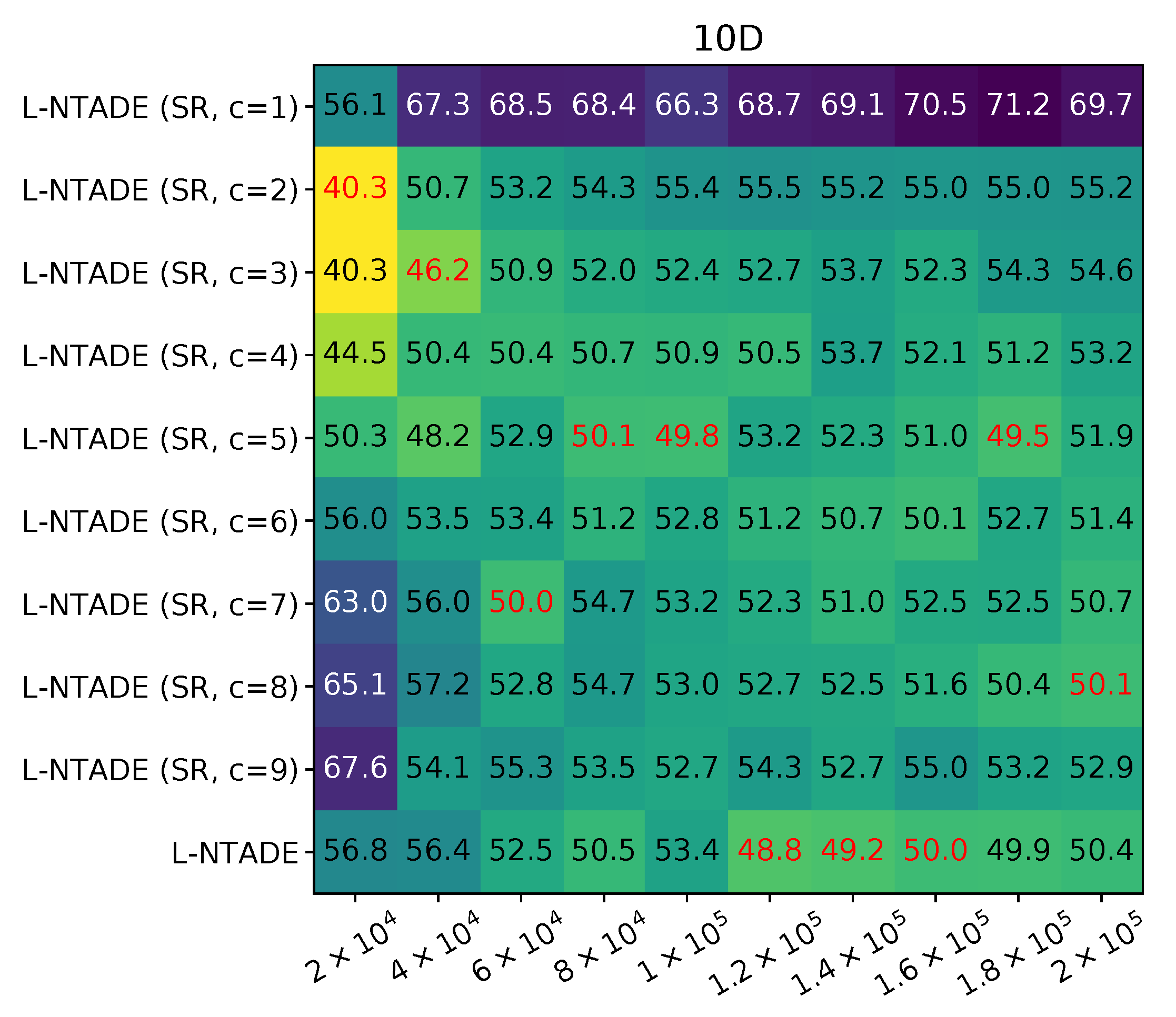
Table 8 contain the results of the L-NTADE algorithm and its modification.
Table 7. L-NTADE (SR) vs. L-NTADE, CEC 2017.
c 10 D 30 D 50 D 100 D
12/10/18 (−105.68)0/8/22 (−192.68)0/4/26 (−218.98)1/2/27 (−219.12)
26/15/9 (−11.94)3/14/13 (−65.01)4/8/18 (−108.84)5/3/22 (−124.60)
39/15/6 (22.08)12/15/3 (43.24)8/17/5 (19.67)8/9/13 (−6.39)
411/14/5 (37.30)14/15/1 (75.39)15/11/4 (69.26)15/11/4 (70.63)
510/16/4 (44.53)14/15/1 (73.95)17/10/3 (67.77)15/11/4 (65.51)
611/17/2 (36.40)9/19/2 (48.88)13/11/6 (25.88)11/12/7 (24.52)
Table 8. L-NTADE (SR) vs. L-NTADE, CEC 2022.
c 10 D 20 D
15/3/4 (11.08)3/2/7 (−22.99)
26/4/2 (25.53)3/3/6 (−6.99)
36/4/2 (25.45)3/5/4 (1.07)
45/5/2 (26.17)2/6/4 (−1.82)
53/8/1 (13.29)2/6/4 (−10.64)
62/6/4 (−10.49)2/7/3 (−12.62)
Although L-NTADE has two populations and has a different algorithmic scheme, applying success rate-based adaptation improved the results in both benchmarks. As before, small c values are inefficient. However, setting c = 4 for CEC 2017 or probably even larger values offers significant performance benefits.
In order to test the applicability of the proposed approach to other algorithms, several of them for which the source codes were available were modified and the modifications were compared to the original results. For the CEC 2017 benchmark, in the jSO (derived from L-SHADE) [25], the mutation step, which uses two factors, F and F 2 , was modified to have only a single one, and the control rules for F were deactivated. For LSHADE-SPACMA [35], the scaling factor sampling in the DE part was replaced by Equation (19). The comparison is shown in Table 9.
Table 9. Comparison of other modified approach vs. original versions, CEC 2017.
Algorithm 10 D 30 D 50 D 100 D
jSO (SR, c = 4 ) vs.1/21/88/16/66/14/1011/9/10
jSO [25](−37.08)(21.04)(−25.27)(−2.29)
LSHADE-SPACMA (SR, c = 4 ) vs.3/22/51/24/50/22/80/23/7
LSHADE-SPACMA [35](−22.61)(−41.67)(−64.32)(−42.11)
As can be seen from Table 9, the modification of jSO with c = 4 may be beneficial in some cases, for example, in the 30D scenario, but in 10D the number of losses was much larger than the number of wins. As for LSHADE-SPACMA, using success rate-based adaptation leads to decreased performance. The main reason why SR-based adaptation failed to improve the performance in these cases could be that both jSO and LSHADE-SPACMA were specifically tuned for the CEC 2017 benchmark, and the SR-based adaptation is a more general approach, which was not tuned for these particular algorithms.
In Table 10, the same modification was applied to APGSK-IMODE (only in IMODE part) [36], MLS-LSHADE [37] and MadDE [38]. Due to a simpler benchmark in terms of computation time, the experiments were performed with different c values.
Table 10. Comparison of other modified approaches vs. original versions, CEC 2022.
Algorithm 10 D 20 D
APGSK-IMODE (SR, c = 2 ) vs.4/5/31/5/6
APGSK-IMODE [36](3.66)(−24.33)
APGSK-IMODE (SR, c = 3 ) vs.4/4/41/8/3
APGSK-IMODE [36](12.88)(−14.19)
APGSK-IMODE (SR, c = 4 ) vs.3/4/51/8/3
APGSK-IMODE [36](−8.81)(−12.24)
APGSK-IMODE (SR, c = 5 ) vs.3/4/51/8/3
APGSK-IMODE [36](−8.81)(−12.24)
MLS-LSHADE (SR, c = 2 ) vs.4/3/50/4/8
MLS-LSHADE [37](−2.05)(−49.53)
MLS-LSHADE (SR, c = 3 ) vs.2/3/70/6/6
MLS-LSHADE [37](−29.50)(−41.34)
MLS-LSHADE (SR, c = 4 ) vs.3/1/80/5/7
MLS-LSHADE [37](−32.78)(−41.91)
MLS-LSHADE (SR, c = 5 ) vs.1/3/80/5/7
MLS-LSHADE [37](−37.41)(−40.96)
MadDE (SR, c = 2 ) vs.5/4/32/6/4
MadDE [38](12.46)(−9.56)
MadDE (SR, c = 3 ) vs.4/5/33/8/1
MadDE [38](14.78)(13.48)
MadDE (SR, c = 4 ) vs.4/5/33/8/1
MadDE [38](13.10)(15.39)
MadDE (SR, c = 5 ) vs.3/6/33/6/3
MadDE [38](4.88)(0.68)
The effect of success rate-based scaling factor adaptation is different for different algorithms. For example, the performance of APGSK-IMODE was improved only in the 10D case, with c = 2 and c = 3 , but for MLS-LSHADE the effect was mainly negative. As for the MadDE algorithm, it was mostly improved by the modification, especially for c = 3 and c = 4 .

4.2.2. Effect of the Available Computational Resource

The main difference between the two considered benchmarks is the number of computations available for every function. The experiments shown above demonstrated that there is a possibility that amount of resource may influence the performance of success rate-based adaptation. To test this hypothesis, a set of experiments was performed for the L-NTADE algorithm on CEC 2022, where the number of function evaluations N F E m a x was decreased to 10 % , 20 % and so on up to 100 % . Figure 2 shows the Friedman ranking of the results in the form of heatmaps.
In Figure 3, the ranking was performed independently in every column, as there is no sense in comparing algorithms with different available resource. The best ranks are shown in red. In the 10 D case, if the resource is relatively small, the success rate adaptation is significantly better than SHA. However, as the N F E m a x grows, the SHA may take the lead. In the 20 D case, however, the SR adaptation is always better, and the best settings are c = 5 or c = 6 , although c = 4 is very similar. From these results, it can be concluded that, first of all, success rate-based adaptation is not highly influenced by available resource, but there is a difference in performance compared to SHA.

4.2.3. Visualization of Parameter Adaptation Process

For a better understanding of what SR actually does during the search process, Figure 4 and Figure 5 show the graphs of F values set by the SHA and SR methods in the case of the L-SHADE-RSP algorithm.
The graphs in Figure 4 show that the behavior of the two considered adaptation methods is quite different, and sometimes even opposite. For example, at the beginning of the search, the success rate is high, and so is the M F value, and they both decrease, while SHA makes larger F values. If the success rate drops close to 0, this makes the M F values oscillate between 0 and 0.5, while SHA slowly tunes values in the memory cells, as seen on functions F15 and F19. If the search process is going well, SR tends to maintain relatively high F values, and switches to an oscillating mode if the success rate is low.
Figure 5 shows similar trends, but they are seen much better due to larger resource. For example, for functions F4, F7 and F8, the success history adaptation leads to memory cell values close to zero at some points in the middle of the search, but success rate adaptation tries every possible F value from 0 to around 0.4 when the success rate drops low. Also, oscillation tends to become higher closer to the end of the search. This is simply the effect of smaller a population size.

4.2.4. Success Rate-Based Adaptation with Different Mutation Strategies

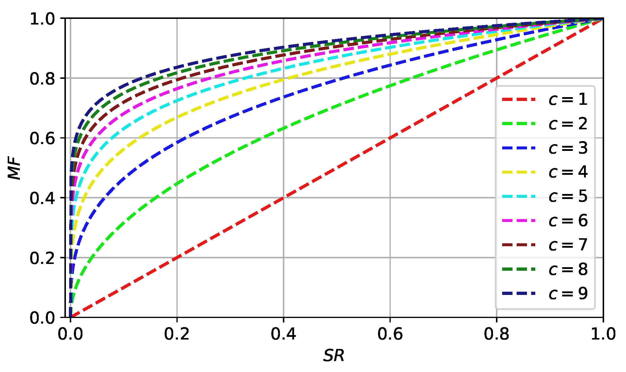
One of the possible explanations of the high performance of success rate-based adaptation for F could be that it works in combination with the current-to-pbest strategy. If the success rate is low, smaller F values force more exploration, while F closer to 1 leads to a move towards one of the p % 
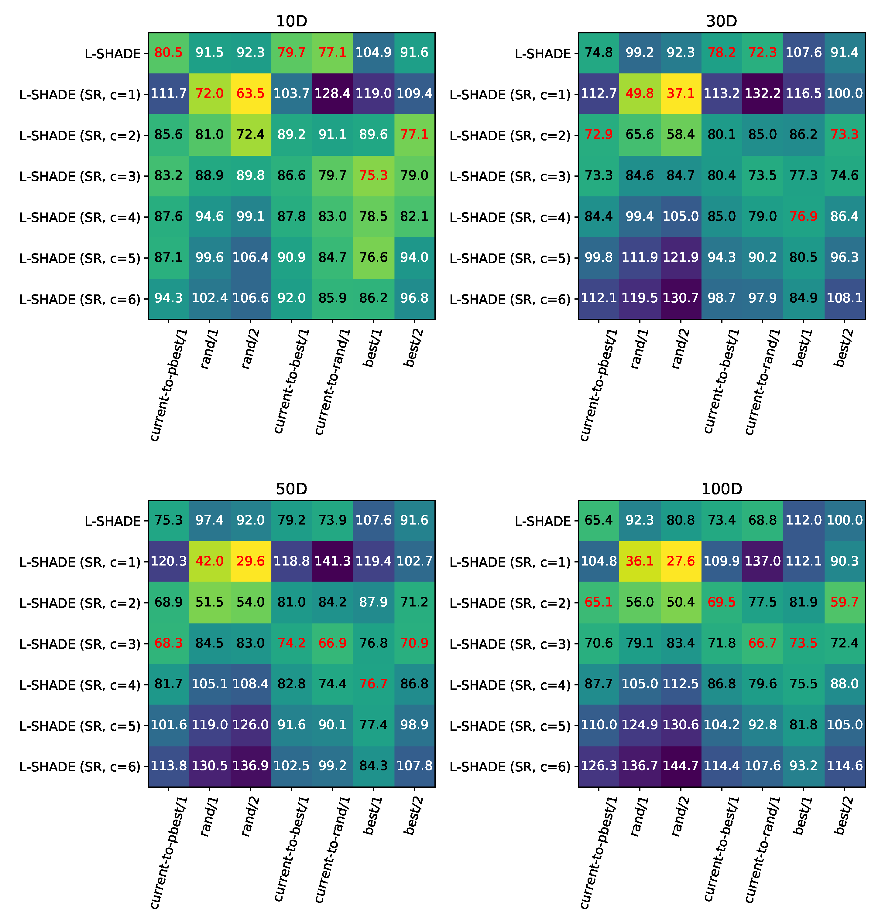
best solutions. To test this effect of success rate-based adaptation, a set of experiments was performed on the standard L-SHADE algorithm with different mutation strategies, such as rand/1, rand/2, current-to-best/1, current-to-rand/1, best/1 and best/2. The c parameter was also altered from 1 to 6, and the original L-SHADE was tested. Next, the Friedman ranking procedure was applied to compare the performance of SHA with SR. The ranks were assigned for each mutation strategy (column) independently. The experiments were repeated for both CEC 2017 and CEC 2022 benchmarks. The parameters of L-SHADE were the following: N = 60 × D 2 3 , p b e s t = 0.2 , H = 5 , initial M F = 0.5 , M C r = 0.5 , archive was not used. Figure 6 and Figure 7 contain the heatmaps of the comparison.
The heatmaps for the CEC 2017 benchmark show that in low-dimensional cases like 10D and 30D, the SHA may perform better than SR, but only for current-to-pbest/1, current-to-best/1 and current-to-rand/1. As for the other strategies, rand/1 and rand/2 performed much better with the modified approach, and so did best/1 and best/2, although the difference here was smaller. In high-dimensional cases, SR is always performing better, especially when the rand/2 strategy is used. Different strategies prefer different c values; for example, rand/1 and rand/2 only use c = 1 , i.e., linear dependence. In fact, this means that the success rate is used directly. Other strategies, such as best/1 and best/2, prefer c = 2 , c = 3 or c = 4 , but this value is always smaller for best/2 compared to best/1. The same is true when comparing rand/1 and rand/2: the effect of smaller c values is larger in the case of rand/2. The current-to-best and current-to-rand strategies are similar to current-to-pbest ones, and the best settings for them are close. The comparison on CEC 2022 demonstrates the same trends, but in general smaller c values are preferred for all strategies except current-to-rand ones. Also, on this benchmark, the SHA is never the best choice.
To compare different strategies with current-to-pbest, the best performing ones from every dimension and every benchmark were chosen and compared to current-to-pbest with SR. The standard SHA was not considered here. The Mann–Whitney statistical tests for both benchmarks are shown in Table 11 and Table 12.
In the case of the CEC 2017 benchmark in Table 11, the current-to-pbest strategy dominates other strategies in terms of performance in all cases. However, the closest competitor is the current-to-best which performed similar in the 50D case, which might indicate a non-optimal choice of the p b e s t parameter for current-to-best. As for the results on CEC 2022, the current-to-pbest outperformed most of the strategies but the current-to-best had several wins in both the 10D and 30D cases. Also, the rand/1 strategy has shown some competitive performance in 20D, as well as best/2 in 10D. Considering the improvements that success rate-based adaptation was able to deliver for these strategies compared to success history adaptation (Figure 6 and Figure 7), one may conclude that SR can be efficiently applied to other strategies, and even make them competitive.

4.2.5. Comparison with Alternative Approaches

Table 13, Table 14 and Table 15 contain the comparison of the L-NTADE (SR) algorithm with c = 4 to other modern DE algorithms on the CEC 2017 benchmark, and Table 16, Table 17 and Table 18 on the CEC 2022 benchmark. Table 13 shows the results of Mann–Whitney statistical tests, Table 14 contains the Friedman ranking results, the ranking that is used in a Friedman statistical test to compare several sets of measurements; smaller total ranks are better. Table 15 shows the recently proposed U-scores [39]. Table 16, Table 17 and Table 18 contain the same results for CEC 2022. The U-scores represent a trial-based dominance method for comparing several optimization methods using Mann–Whitney U tests. For CEC 2017, the convergence speed is not taken into consideration, while for CEC 2022 the number of function evaluations to reach the desired accuracy is considered.
As can be seen from Table 13, the L-NTADE algorithm with success rate-based adaptation is able to outperform most of the alternative algorithms in both benchmarks. EBOwithCMAR performed better in the 10D case, and LSHADE-SPACMA showed comparable in the 100D case. Table 14 supports these results, ranking L-NTADE with c = 4 the best algorithm overall, and even the standard L-NTADE is very competitive. In Table 15, the comparison yields similar results, and L-NTADE with c = 4 ranks first, followed by LSHADE-SPACMA and L-NTADE.
Table 15. L-NTADE (SR) vs. alternative approaches, U-scores. Larger ranks are better [39], CEC 2017.
Algorithm 10 D 30 D -
LSHADE-SPACMA [35]263,193293,839.5-
jSO [25]272,469282,122.5-
EBOwithCMAR [40]322,146.5303,458.5-
L-SHADE-RSP [9]276,570.5296,012-
NL-SHADE-RSP [10]244,170112,109-
NL-SHADE-LBC [11]276,146161,327-
L-NTADE [12]248,186336,712.5-
L-NTADE (SR, c = 4 )281,959399,259-
Algorithm 50 D 100 D Total
LSHADE-SPACMA [35]364,005.5404,6531,325,691
jSO [25]281,506262,6311,098,728.5
EBOwithCMAR [40]298,859282,2271,206,691
L-SHADE-RSP [9]305,628.5305,8171,184,028
NL-SHADE-RSP [10]34,664.534,687425,630.5
NL-SHADE-LBC [11]121,800.5124,111683,384.5
L-NTADE [12]362,005359,2211,306,124.5
L-NTADE (SR, c = 4 )416,371411,4931,509,082
Table 16. L-NTADE (SR) vs. alternative approaches, CEC 2022.
Algorithm 10 D 20 D
L-NTADE (SR, c = 4 ) vs.8/2/210/0/2
APGSK-IMODE [36](36.86)(52.60)
L-NTADE (SR, c = 4 ) vs.4/2/64/1/7
MLS-LSHADE [37](−9.67)(−19.78)
L-NTADE (SR, c = 4 ) vs.8/2/28/2/2
MadDE [38](39.05)(43.60)
L-NTADE (SR, c = 4 ) vs.2/6/45/3/4
EA4eigN100 [41](−15.49)(5.51)
L-NTADE (SR, c = 4 ) vs.3/4/56/2/4
NL-SHADE-RSP-MID [42](−5.98)(17.59)
L-NTADE (SR, c = 4 ) vs.5/3/44/6/2
L-SHADE-RSP [9](14.23)(12.24)
L-NTADE (SR, c = 4 ) vs.6/3/37/4/1
NL-SHADE-RSP [10](24.51)(34.78)
L-NTADE (SR, c = 4 ) vs.2/3/74/4/4
NL-SHADE-LBC [11](−30.20)(−3.75)
L-NTADE (SR, c = 4 ) vs.5/5/22/6/4
L-NTADE [12](26.17)(−1.82)
The comparison on the CEC 2022 benchmark in Table 16 shows that L-NTADE with c = 4 is outperformed by NL-SHADE-LBC and EA4eigN100 in the 10D case, but in 20D the difference between them decreases. However, the MLS-LSHADE is able to deliver better performance in the 20D case. The Friedman ranking in Table 17 sets EA4eigN100 in first place, followed by NL-SHADE-LBC, and MLS-LSHADE and L-NTADE with c = 4 . However, when using U-scores in Table 18, L-NTADE with c = 4 takes second place after NL-SHADE-LBC, and MLS-LSHADE has an almost identical total rank. We note that L-NTADE used the same parameter settings in both benchmarks, and still was able to show highly competitive results in both of them.
Table 17. L-NTADE (SR) vs. alternative approaches, Friedman ranking. Smaller ranks are better, CEC 2022.
Algorithm 10 D 20 D Total
APGSK-IMODE [36]81.5787.92169.48
MLS-LSHADE [37]64.0550.13114.18
MadDE [38]87.1587.02174.17
EA4eigN100 [41]39.1753.0292.18
NL-SHADE-RSP-MID [42]58.9271.25130.17
L-SHADE-RSP [9]66.6559.07125.72
NL-SHADE-RSP [10]88.2383.58171.82
NL-SHADE-LBC [11]49.7756.73106.50
L-NTADE [12]64.5855.92120.50
L-NTADE (SR, c = 4 )59.9255.37115.28
Table 18. L-NTADE (SR) vs. alternative approaches, U-scores. Larger ranks are better [39], CEC 2022.
Algorithm 10 D 20 D Total
APGSK-IMODE [36]38,22828,381.566,609.5
MLS-LSHADE [37]52,25562,548.5114,803.5
MadDE [38]35,72730,402.566,129.5
EA4eigN100 [41]5035860,202110,560
NL-SHADE-RSP-MID [42]56,740.544,291.5101,032
L-SHADE-RSP [9]44,754.554,543.599,298
NL-SHADE-RSP [10]35,363.532,772.568,136
NL-SHADE-LBC [11]64,33056,998.5121,328.5
L-NTADE [12]51,34657,894109,240
L-NTADE (SR, c = 4 )56,897.557,965.5114,863
In order to compare the computational complexity of the proposed approach, the experiment on the CEC 2022 benchmark was performed according to the rules of the CEC 2022 competition rules [14]. The T0, T1 and T2 values are the estimations of time required for the processor to perform mathematical evaluations, target function evaluation time and the algorithm runtime, respectively. Table 19 compares L-NTADE with the SHA and the SR adaptation methods.
As can be seen from Table 19, applying SR reduces the amount of time, as the calculation of the weighted Lehmer mean for F in success history-based adaptation requires significant computational effort.

5. Discussion

The main advantage of the proposed success rate-based adaptation of the scaling factor is its simplicity. As simple as the original DE, it relies on a naturally present value in the algorithm, namely the number of successful individuals, i.e., the number of solutions that were improved according to the selection step. This number is, in fact, calculated by the majority of existing DE algorithms. Success rate-based adaptation does not require complex calculations of means, averaging over time and other techniques, and still performs very well. Moreover, the experiments have shown that the sensitivity to the c parameter is very low: the same value, c = 4 , works on different benchmarks, different functions and different computational resource. This property makes for a universal approach, which seems to work well enough in most scenarios. Although there are cases when the success history adaptation may deliver better performance, we believe that this can be mitigated by further development of SR-based adaptation schemes.
As for the reasons for high performance, and why c = 4 is a good choice in many cases, the following explanation seems reasonable. The SR in most tested algorithms worked together with the current-to-pbest mutation strategy, which has a specific structure. If F > 0.5 , then the new solutions are attracted closer to some of the best ones, although this also means that larger steps in other directions will be made. If F < 0.5 , this means that the attention towards better solutions is smaller, and the algorithm searches more around the current positions of each individual. What the success rate adaptation does is it switches between these two behaviors. If the search is going well, it makes DE generate solutions closer to better ones, and the F values are relatively stable. However, if the algorithm is stagnating, a wider search is beneficial. In this case, success rate adaptation makes M F oscillate in the [ 0 , 0.5 ] range, sampling smaller F values and trying to escape local optima. In this manner, applying a simple curve like S R 1 / 4 produces the desired behavior of DE without complex adaptation mechanisms.
The experiments with other mutation strategies revealed that SR-based adaptation works not only with the current-to-pbest strategy, but also with other ones, and in all cases there was a setting of c which lead to improved performance. Moreover, in most cases, any c value resulted in better performance than SHA. In the case of the rand/1 and rand/2 strategies, this improvement was very significant, and even allowed for current-to-pbest to be outperformed in some cases. This might mean that the SR-based adaptation can be used as a universal mechanism, independent of the mutation strategy, although the c value should be set accordingly.
Replacing the original success history adaptation in other DE-based algorithms, such as APGSK-IMODE, MLS-LSHADE, MadDE, jSO and LSHADE-SPACMA, did not always improve performance; nevertheless, the results were mostly comparable. Some of the modified algorithms represented hybrids with other methods, such as local search or covariance matrix adaptation, and probably better results could be achieved with a more careful tuning of the hybridization.
Of course, the presented experiments cannot cover all the possibilities of success rate-based adaptation. However, it is worth mentioning some of the possible directions of further studies, which include:
  • Developing a crossover rate adaptation scheme based on the success rate,
  • Connecting the success rate to the p b e s t parameter,
  • Combining the advantages of the success history and success rate adaptation.

6. Conclusions

In this study, a new adaptation technique for the scaling factor parameter in differential evolution was proposed. The new method relies on the success rate, and the performed experimental analysis showed that the new method is insensitive to computational resource, works with different mutation strategies, and can be included in various algorithms.

Author Contributions

Conceptualization, V.S. and E.S.; methodology, V.S. and E.S.; software, V.S.; validation, V.S. and E.S.; formal analysis, E.S.; investigation, V.S.; resources, E.S. and V.S.; data curation, E.S.; writing—original draft preparation, V.S.; writing—review and editing, V.S.; visualization, V.S.; supervision, E.S.; project administration, E.S.; funding acquisition, V.S. and E.S. All authors have read and agreed to the published version of the manuscript.

Funding

This work was supported by the Ministry of Science and Higher Education of the Russian Federation within limits of state contract No. FEFE-2023-0004.

Data Availability Statement

Data are contained within the article.

Conflicts of Interest

The authors declare no conflict of interest.

Abbreviations

The following abbreviations are used in this manuscript:
GAGenetic Algorithms
GPGenetic Programming
ECEvolutionary Computation
DEDifferential Evolution
CECCongress on Evolutionary Computation
SHADESuccess History Adaptive Differential Evolution
LPSRLinear Population Size Reduction
LBCLinear Bias Change
RSPRank-based Selective Pressure
L-NTADELinear population size reduction Newest and Top Adaptive Differential Evolution

References

  1. Price, K.; Storn, R.; Lampinen, J. Differential Evolution: A Practical Approach to Global Optimization; Springer: Berlin/Heidelberg, Germany, 2005. [Google Scholar]
  2. Das, S.; Suganthan, P. Differential evolution: A survey of the state-of-the-art. IEEE Trans. Evol. Comput. 2011, 15, 4–31. [Google Scholar] [CrossRef]
  3. Brest, J.; Greiner, S.; Boškovic, B.; Mernik, M.; Žumer, V. Self-adapting control parameters in differential evolution: A comparative study on numerical benchmark problems. IEEE Trans. Evol. Comput. 2006, 10, 646–657. [Google Scholar] [CrossRef]
  4. Zhang, J.; Sanderson, A.C. JADE: Adaptive Differential Evolution with Optional External Archive. IEEE Trans. Evol. Comput. 2009, 13, 945–958. [Google Scholar] [CrossRef]
  5. Tanabe, R.; Fukunaga, A. Success-history based parameter adaptation for differential evolution. In Proceedings of the 2013 IEEE Congress on Evolutionary Computation, Cancun, Mexico, 20–23 June 2013; pp. 71–78. [Google Scholar] [CrossRef]
  6. Piotrowski, A.P.; Napiorkowski, J.J. Step-by-step improvement of JADE and SHADE-based algorithms: Success or failure? Swarm Evol. Comput. 2018, 43, 88–108. [Google Scholar] [CrossRef]
  7. Stanovov, V.; Akhmedova, S.; Semenkin, E. Biased Parameter Adaptation in Differential Evolution. Inf. Sci. 2021, 566, 215–238. [Google Scholar] [CrossRef]
  8. Stanovov, V.; Akhmedova, S.; Semenkin, E. The automatic design of parameter adaptation techniques for differential evolution with genetic programming. Knowl. Based Syst. 2022, 239, 108070. [Google Scholar] [CrossRef]
  9. Stanovov, V.; Akhmedova, S.; Semenkin, E. LSHADE Algorithm with Rank-Based Selective Pressure Strategy for Solving CEC 2017 Benchmark Problems. In Proceedings of the 2018 IEEE Congress on Evolutionary Computation (CEC), Rio de Janeiro, Brazil, 8–13 July 2018; pp. 1–8. [Google Scholar]
  10. Stanovov, V.; Akhmedova, S.; Semenkin, E. NL-SHADE-RSP Algorithm with Adaptive Archive and Selective Pressure for CEC 2021 Numerical Optimization. In Proceedings of the 2021 IEEE Congress on Evolutionary Computation (CEC), Kraków, Poland, 28 June–1 July 2021; pp. 809–816. [Google Scholar] [CrossRef]
  11. Stanovov, V.; Akhmedova, S.; Semenkin, E. NL-SHADE-LBC algorithm with linear parameter adaptation bias change for CEC 2022 Numerical Optimization. In Proceedings of the 2022 IEEE Congress on Evolutionary Computation (CEC), Padua, Italy, 18–23 July 2022. [Google Scholar]
  12. Stanovov, V.; Akhmedova, S.; Semenkin, E. Dual-Population Adaptive Differential Evolution Algorithm L-NTADE. Mathematics 2022, 10, 4666. [Google Scholar] [CrossRef]
  13. Awad, N.; Ali, M.; Liang, J.; Qu, B.; Suganthan, P. Problem Definitions and Evaluation Criteria for the CEC 2017 special Session and Competition on Single Objective Bound Constrained Real-Parameter Numerical Optimization; Technical Report; Nanyang Technological University: Singapoure, 2016. [Google Scholar]
  14. Kumar, A.; Price, K.; Mohamed, A.K.; Suganthan, P.N. Problem Definitions and Evaluation Criteria for the CEC 2022 Special Session and Competition on Single Objective Bound Constrained Numerical Optimization; Technical Report; Nanyang Technological University: Singapoure, 2021. [Google Scholar]
  15. Storn, R.; Price, K. Differential evolution—A simple and efficient heuristic for global optimization over continuous spaces. J. Glob. Optim. 1997, 11, 341–359. [Google Scholar] [CrossRef]
  16. Biedrzycki, R.; Arabas, J.; Jagodziński, D. Bound constraints handling in Differential Evolution: An experimental study. Swarm Evol. Comput. 2019, 50, 100453. [Google Scholar] [CrossRef]
  17. Kumar, A.; Biswas, P.P.; Suganthan, P.N. Differential evolution with orthogonal array-based initialization and a novel selection strategy. Swarm Evol. Comput. 2022, 68, 101010. [Google Scholar] [CrossRef]
  18. Das, S.; Mullick, S.; Suganthan, P. Recent advances in differential evolution—An updated survey. Swarm Evol. Comput. 2016, 27, 1–30. [Google Scholar] [CrossRef]
  19. Al-Dabbagh, R.D.; Neri, F.; Idris, N.; Baba, M.S.B. Algorithmic design issues in adaptive differential evolution schemes: Review and taxonomy. Swarm Evol. Comput. 2018, 43, 284–311. [Google Scholar] [CrossRef]
  20. Brest, J.; Maucec, M.; Bovsković, B. The 100-Digit Challenge: Algorithm jDE100. In Proceedings of the 2019 IEEE Congress on Evolutionary Computation (CEC), Wellington, New Zealand, 10–13 June 2019; pp. 19–26. [Google Scholar]
  21. Brest, J.; Maucec, M.; Bosković, B. Differential Evolution Algorithm for Single Objective Bound-Constrained Optimization: Algorithm j2020. In Proceedings of the 2020 IEEE Congress on Evolutionary Computation (CEC), Glasgow, UK, 19–24 July 2020; pp. 1–8. [Google Scholar]
  22. Qin, A.K.; Suganthan, P.N. Self-adaptive differential evolution algorithm for numerical optimization. In Proceedings of the 2005 IEEE Congress on Evolutionary Computation, Edinburgh, UK, 2–5 September 2005; Volume 2, pp. 1785–1791. [Google Scholar]
  23. Bullen, P. Handbook of Means and Their Inequalities; Springer: Amsterdam, The Netherlands, 2003. [Google Scholar] [CrossRef]
  24. Tanabe, R.; Fukunaga, A. Improving the search performance of SHADE using linear population size reduction. In Proceedings of the IEEE Congress on Evolutionary Computation, CEC, Beijing, China, 6–11 July 2014; pp. 1658–1665. [Google Scholar] [CrossRef]
  25. Brest, J.; Maučec, M.; Boškovic, B. Single objective real-parameter optimization algorithm jSO. In Proceedings of the IEEE Congress on Evolutionary Computation, Donostia, Spain, 5–8 June 2017; pp. 1311–1318. [Google Scholar] [CrossRef]
  26. Gong, W.; Cai, Z. Differential Evolution With Ranking-Based Mutation Operators. IEEE Trans. Cybern. 2013, 43, 2066–2081. [Google Scholar] [CrossRef] [PubMed]
  27. Viktorin, A.; Senkerik, R.; Pluhacek, M.; Kadavy, T.; Zamuda, A. Distance based parameter adaptation for Success-History based Differential Evolution. Swarm Evol. Comput. 2019, 50, 100462. [Google Scholar] [CrossRef]
  28. Bujok, P.; Kolenovsky, P. Differential Evolution with Distance-based Mutation-selection Applied to CEC 2021 Single Objective Numerical Optimisation. In Proceedings of the 2021 IEEE Congress on Evolutionary Computation (CEC), Kraków, Poland, 28 June–1 July 2021; pp. 849–856. [Google Scholar]
  29. Yang, M.; Cai, Z.; Li, C.; Guan, J. An improved adaptive differential evolution algorithm with population adaptation. In Proceedings of the Annual Conference on Genetic and Evolutionary Computation, Amsterdam, The Netherlands, 6–10 July 2013. [Google Scholar]
  30. Santucci, V.; Baioletti, M.; Bari, G.D. An improved memetic algebraic differential evolution for solving the multidimensional two-way number partitioning problem. Expert Syst. Appl. 2021, 178, 114938. [Google Scholar] [CrossRef]
  31. Chen, X.; Shen, A. Self-adaptive differential evolution with Gaussian–Cauchy mutation for large-scale CHP economic dispatch problem. Neural Comput. Appl. 2022, 34, 11769–11787. [Google Scholar] [CrossRef]
  32. Yi, W.; Chen, Y.; Pei, Z.; Lu, J. Adaptive differential evolution with ensembling operators for continuous optimization problems. Swarm Evol. Comput. 2021, 69, 100994. [Google Scholar] [CrossRef]
  33. Yang, Q.; Qiao, Z.Y.; Xu, P.; Lin, X.; Gao, X.D.; Wang, Z.J.; Lu, Z.Y.; Jeon, S.W.; Zhang, J. Triple competitive differential evolution for global numerical optimization. Swarm Evol. Comput. 2024, 84, 101450. [Google Scholar] [CrossRef]
  34. Kitamura, T.; Fukunaga, A. Differential Evolution with an Unbounded Population. In Proceedings of the 2022 IEEE Congress on Evolutionary Computation (CEC), Padua, Italy, 18–23 July 2022. [Google Scholar]
  35. Mohamed, A.; Hadi, A.A.; Fattouh, A.; Jambi, K. LSHADE with semi-parameter adaptation hybrid with CMA-ES for solving CEC 2017 benchmark problems. In Proceedings of the 2017 IEEE Congress on Evolutionary Computation (CEC), Donostia, Spain, 5–8 June 2017; pp. 145–152. [Google Scholar]
  36. Mohamed, A.W.; Hadi, A.A.; Agrawal, P.; Sallam, K.M.; Mohamed, A.K. Gaining-Sharing Knowledge Based Algorithm with Adaptive Parameters Hybrid with IMODE Algorithm for Solving CEC 2021 Benchmark Problems. In Proceedings of the 2021 IEEE Congress on Evolutionary Computation (CEC), Kraków, Poland, 28 June–1 July 2021; pp. 841–848. [Google Scholar]
  37. Cuong, L.V.; Bao, N.N.; Binh, H.T.T. Technical Report: A Multi-Start Local Search Algorithm with L-SHADE for Single Objective Bound Constrained Optimization; Technical Report; SoICT, Hanoi University of Science and Technology: Hanoi, Vietnam, 2021. [Google Scholar]
  38. Biswas, S.; Saha, D.; De, S.; Cobb, A.D.; Das, S.; Jalaian, B. Improving Differential Evolution through Bayesian Hyperparameter Optimization. In Proceedings of the 2021 IEEE Congress on Evolutionary Computation (CEC), Kraków, Poland, 28 June–1 July 2021; pp. 832–840. [Google Scholar]
  39. Price, K.V.; Kumar, A.; Suganthan, P. Trial-based dominance for comparing both the speed and accuracy of stochastic optimizers with standard non-parametric tests. Swarm Evol. Comput. 2023, 78, 101287. [Google Scholar] [CrossRef]
  40. Kumar, A.; Misra, R.K.; Singh, D. Improving the local search capability of Effective Butterfly Optimizer using Covariance Matrix Adapted Retreat Phase. In Proceedings of the 2017 IEEE Congress on Evolutionary Computation (CEC), Donostia, Spain, 5–8 June 2017; pp. 1835–1842. [Google Scholar]
  41. Bujok, P.; Kolenovsky, P. Eigen Crossover in Cooperative Model of Evolutionary Algorithms Applied to CEC 2022 Single Objective Numerical Optimisation. In Proceedings of the 2022 IEEE Congress on Evolutionary Computation (CEC), Padua, Italy, 18–23 July 2022. [Google Scholar]
  42. Biedrzycki, R.; Arabas, J.; Warchulski, E. A Version of NL-SHADE-RSP Algorithm with Midpoint for CEC 2022 Single Objective Bound Constrained Problems. In Proceedings of the 2022 IEEE Congress on Evolutionary Computation (CEC), Padua, Italy, 18–23 July 2022. [Google Scholar]
Figure 1. M F values for different c parameter values.
Mathematics 12 00516 g001
Figure 2. Comparison of steps required for success rate-based adaptation and success history-based adaptation.
Mathematics 12 00516 g002
Figure 3. Comparison of L-NTADE with and without success rate adaptation with different available resource N F E m a x , Friedman ranking.
Mathematics 12 00516 g003aMathematics 12 00516 g003b
Figure 4. Graphs of parameter adaptation of L-SHADE-RSP with and without success rate adaptation, CEC 2017, 30 D , selected functions.
Mathematics 12 00516 g004
Figure 5. Graphs of parameter adaptation of L-SHADE-RSP with and without success rate adaptation, CEC 2022, 20 D .
Mathematics 12 00516 g005
Figure 6. Comparison of L-SHADE with different strategies, with and without success rate adaptation, CEC 2017, Friedman ranking.
Mathematics 12 00516 g006
Figure 7. Comparison of L-SHADE with different strategies, with and without success rate adaptation, CEC 2022, Friedman ranking.
Mathematics 12 00516 g007
Table 1. L-SHADE-RSP (SR) vs. L-SHADE-RSP, CEC 2017.
c 10 D 30 D 50 D 100 D
13/18/9 (−45.16)0/9/21 (−157.01)0/7/23 (−163.79)2/5/23 (−183.13)
23/23/4 (−12.68)4/11/15 (−74.72)4/8/18 (−87.52)4/9/17 (−91.82)
35/23/2 (4.32)5/16/9 (−28.41)5/15/10 (−25.87)8/12/10 (−16.28)
44/26/0 (19.57)2/23/5 (−18.11)5/20/5 (2.37)11/11/8 (11.60)
55/23/2 (14.58)3/20/7 (−31.34)1/25/4 (−11.09)12/10/8 (16.57)
66/19/5 (8.65)2/18/10 (−41.83)3/20/7 (−33.75)12/11/7 (4.25)
Table 2. L-SHADE-RSP (SR) vs. L-SHADE-RSP, CEC 2022.
c 10 D 20 D
17/3/2 (29.61)3/3/6 (−11.30)
27/3/2 (30.91)4/4/4 (4.29)
36/3/3 (21.43)4/6/2 (18.58)
44/2/6 (−8.13)2/8/2 (−3.00)
54/4/4 (−8.23)2/6/4 (−14.21)
63/5/4 (−9.17)1/7/4 (−16.18)
Table 11. L-SHADE (SR) with different mutation strategies, current-to-pbest strategy vs. best variants, CEC 2017.
Strategy 10 D 30 D 50 D 100 D
current-to-pbest/1 vs.10/11/919/9/224/4/218/8/4
rand/1(26.18)(110.36)(150.35)(133.91)
current-to-pbest/1 vs.11/16/320/9/125/3/220/6/4
rand/2(56.51)(134.71)(174.02)(146.97)
current-to-pbest/1 vs.15/10/55/22/34/22/411/10/9
current-to-best/1(45.26)(17.98)(3.20)(19.94)
current-to-pbest/1 vs.11/17/219/11/019/9/222/7/1
current-to-rand/1(52.97)(119.34)(135.04)(164.06)
current-to-pbest/1 vs.9/17/415/11/423/4/320/6/4
best/1(20.28)(80.90)(108.31)(107.48)
current-to-pbest/1 vs.11/16/317/11/224/4/220/6/4
best/2(27.58)(80.53)(123.93)(108.48)
Table 12. L-SHADE (SR) with different mutation strategies, current-to-pbest strategy vs. best variants, CEC 2022.
Strategy 10 D 20 D
current-to-pbest/1 vs. rand/14/5/3 (1.77)3/5/4 (−5.97)
current-to-pbest/1 vs. rand/24/5/3 (8.87)2/7/3 (−1.72)
current-to-pbest/1 vs. current-to-best/11/7/4 (−15.58)1/8/3 (−8.00)
current-to-pbest/1 vs. current-to-rand/17/4/1 (35.73)5/6/1 (22.00)
current-to-pbest/1 vs. best/15/3/4 (1.91)5/4/3 (12.18)
current-to-pbest/1 vs. best/23/4/5 (−10.48)6/2/4 (13.10)
Table 13. L-NTADE (SR) vs. alternative approaches, Mann–Whitney tests, CEC 2017.
Algorithm 10 D 30 D 50 D 100 D
L-NTADE (SR, c = 4 ) vs.9/18/317/6/714/3/1314/1/15
LSHADE-SPACMA [35](25.76)(75.97)(17.98)(1.50)
L-NTADE (SR, c = 4 ) vs.6/21/319/10/122/6/224/1/5
jSO [25](7.27)(139.25)(153.40)(147.83)
L-NTADE (SR, c = 4 ) vs.3/19/816/9/518/7/522/2/6
EBOwithCMAR [40](−37.99)(79.00)(110.30)(131.61)
L-NTADE (SR, c = 4 ) vs.3/24/318/11/120/8/220/6/4
L-SHADE-RSP [9](2.69)(127.15)(131.90)(121.52)
L-NTADE (SR, c = 4 ) vs.12/9/923/4/329/1/029/0/1
NL-SHADE-RSP [10](17.82)(173.49)(250.21)(241.25)
L-NTADE (SR, c = 4 ) vs.6/20/421/8/128/2/027/1/2
NL-SHADE-LBC [11](6.58)(176.68)(227.05)(210.08)
L-NTADE (SR, c = 4 ) vs.11/14/514/15/115/11/415/11/4
L-NTADE [12](37.30)(75.39)(69.26)(70.63)
Table 14. L-NTADE (SR) vs. alternative approaches; Friedman ranking. Smaller ranks are better, CEC 2017.
Algorithm 10 D 30 D 50 D 100 D Total
LSHADE-SPACMA [35]139.42127.42100.5585.06452.45
jSO [25]134.97131.33132.14139.09537.53
EBOwithCMAR [40]116.15123.19124.94131.67495.94
L-SHADE-RSP [9]133.93126.37121.91122.36504.58
NL-SHADE-RSP [10]146.25196.87226.37226.63796.13
NL-SHADE-LBC [11]133.80177.80193.38191.89696.88
L-NTADE [12]143.55110.41100.85101.93456.75
L-NTADE (SR, c = 4 )131.9286.6079.8581.37379.75
Table 19. Computational complexity of L-NTADE with SHA and the SR adaptation methods.
L-NTADE
D T 0 T 1 T 2 ( T 2 T 1 ) / T 0
D = 10 2.5 × 10−22.1 × 10−21.358 × 10−14.592
D = 20 2.5 × 10−25.0 × 10−21.704 × 10−14.816
L-NTADE (SR, c = 4 )
D T 0 T 1 T 2 ( T 2 T 1 ) / T 0
D = 10 2.5 × 10−22.1 × 10−21.192 × 10−13.928
D = 20 2.5 × 10−25.0 × 10−21.658 × 10−14.632
Disclaimer/Publisher’s Note: The statements, opinions and data contained in all publications are solely those of the individual author(s) and contributor(s) and not of MDPI and/or the editor(s). MDPI and/or the editor(s) disclaim responsibility for any injury to people or property resulting from any ideas, methods, instructions or products referred to in the content.

